
Bearing Fault Diagnosis Based on Stochastic Resonance and Improved Whale Optimization Algorithm


Abstract
:1. Introduction
2. Parameter-Adaptive Stochastic Resonance
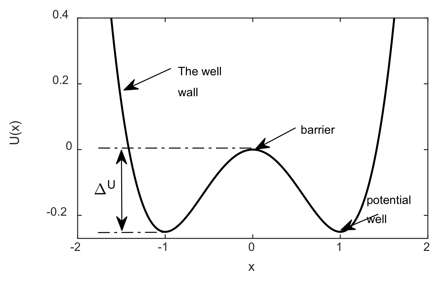
2.1. Bistable Stochastic Resonance
2.2. Determination of Parameter Ranges
3. Improved Whale Optimization Algorithm
3.1. WOA
3.2. Improved Whale Optimization Algorithm
3.2.1. Chaos Sequence Initialization
3.2.2. Linear Time-Varying Factors and Adaptive Weights
3.2.3. Random Learning Strategy
3.2.4. Cauchy Mutation Strategy
4. Stochastic Resonance Parameter Adaptive Strategy
4.1. Stochastic Resonance Parameter Adaptation Based on Improved Whale Optimization Algorithm
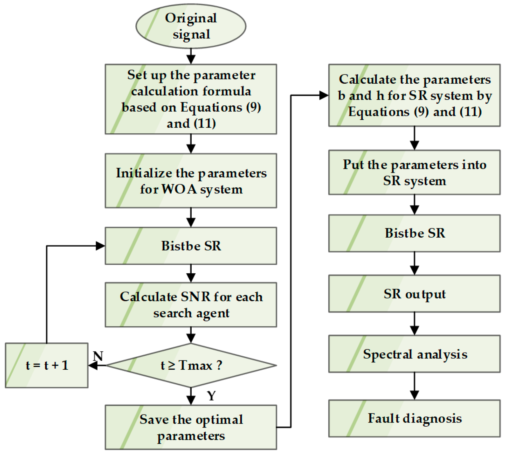
- Step 1:
- Input the noisy signal, establish the calculation process of Formulas (9) and (11), and initialize the parameters of the whale optimization system. The value ranges of , , and are [0, 0.5], [0, 1], [0, 10], respectively. The maximum iteration time is 200 and the whale population is 30.
- Step 2:
- Optimize SR parameters through IWOA and calculate the SNR. Update the best position for particles until the maximum number of iterations.
- Step 3:
- Obtain the optimal solution of , , by IWOA. Then the parameters and are calculated according to Equations (9) and (11).
- Step 4:
- Substitute , , into the stochastic resonance system to run, and convert the calculation results into the frequency domain through Fourier transform. Diagnose the fault signal by analyzing the results of the frequency domain.
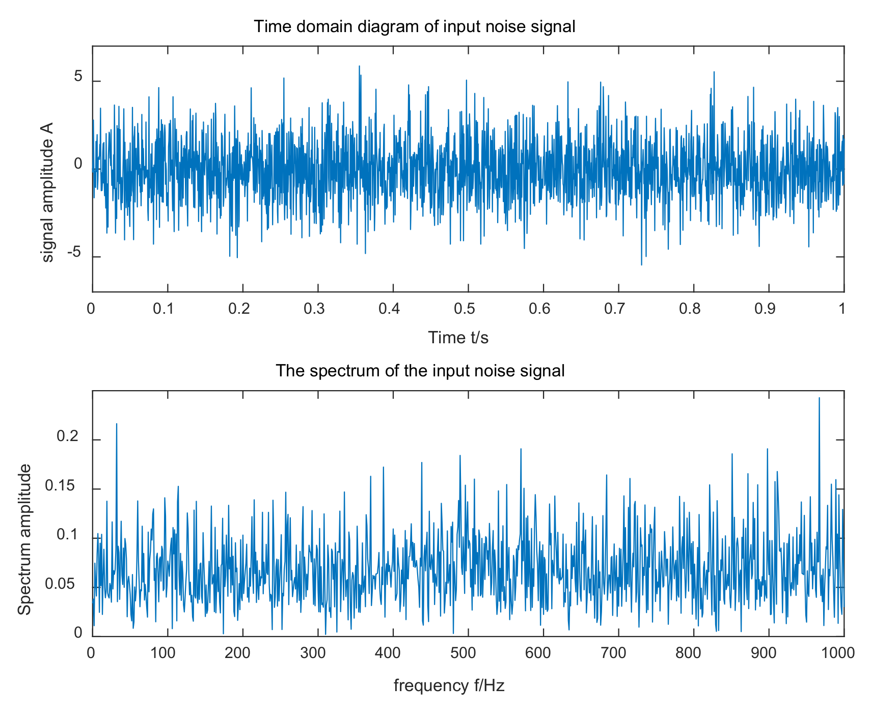
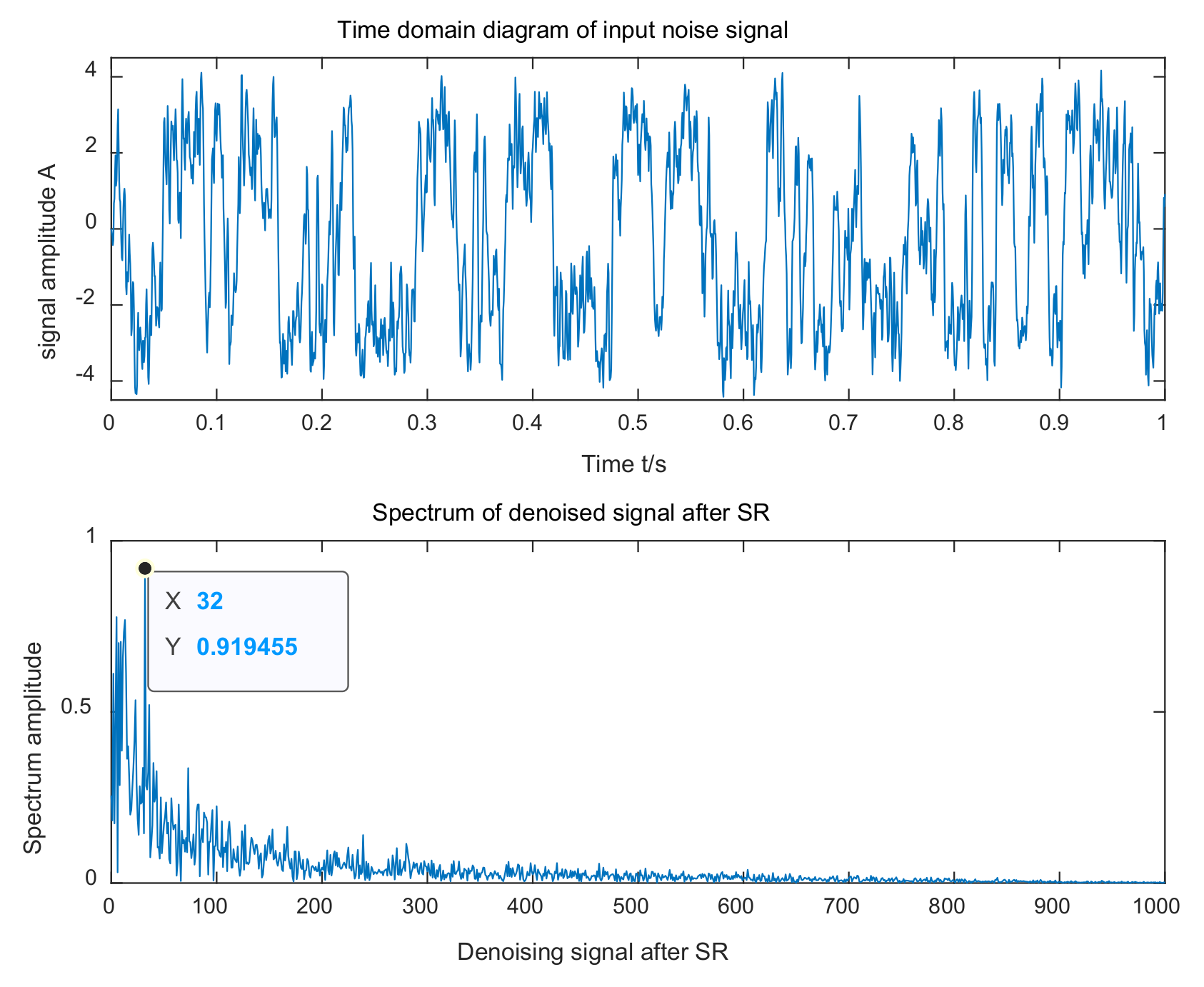
4.2. Simulation
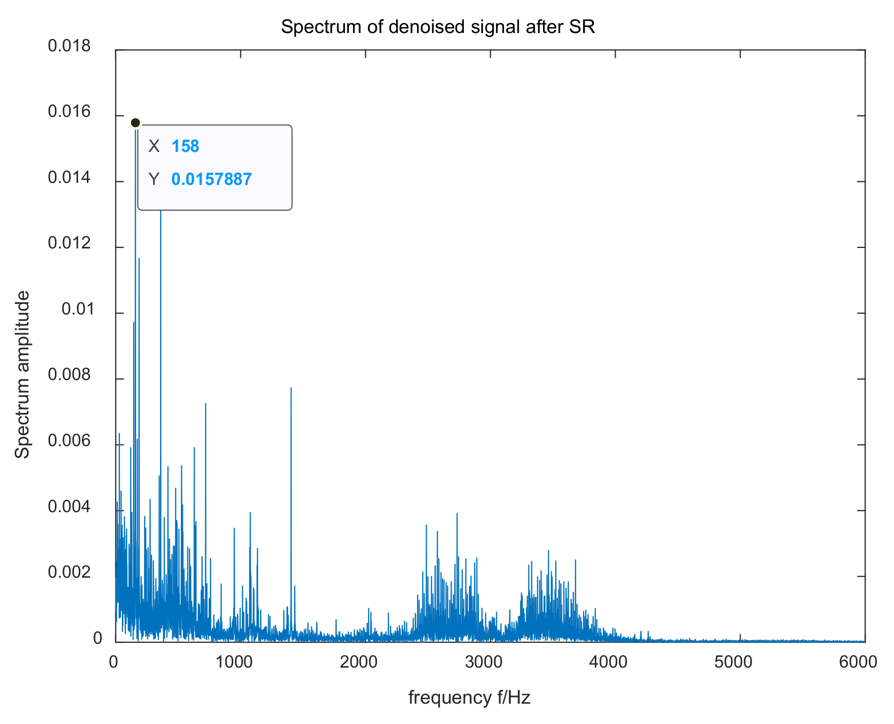
5. Bearing Fault Detection Experiment
5.1. Bearing Fault Detection Based on IWOA
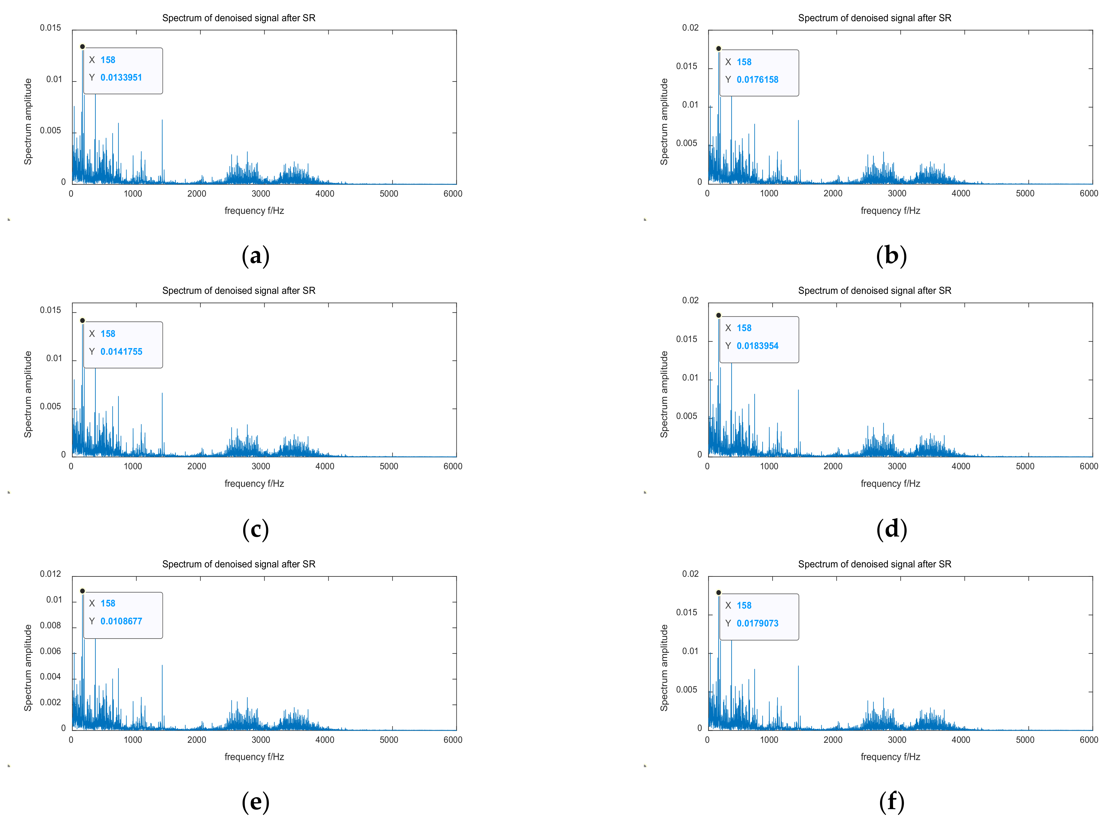
5.2. Comparison with Other Methods
6. Conclusions
Author Contributions
Funding
Informed Consent Statement
Data Availability Statement
Conflicts of Interest
References
- Tyagi, S.; Panigrahi, S.K. A Simple Continuous Wavelet Transform Method for Rolling Bearing Fault Detection and Its Comparison with Envelope Detection. J. Res. Sci. Eng. 2021, 3, 1033–1040. [Google Scholar]
- Waters, W.M.; Jarrett, B.R. Bandpass Signal Sampling and Coherent Detection. IEEE Trans. Aerosp. Electron. Syst. 1982, 18, 731–736. [Google Scholar] [CrossRef]
- Lu, C.; Gao, L.; Li, X.Y.; Hu, C.Y.; Yan, X.S.; Gong, W.Y. Chaotic-based grey wolf optimizer for numerical and engineering optimization problems. Memetic Comput. 2020, 12, 371–398. [Google Scholar] [CrossRef]
- Mahata, S.; Shakya, P.; Babu, N.R. A robust condition monitoring methodology for grinding wheel wear identification using Hilbert Huang transform. Precis. Eng. 2021, 70, 77–91. [Google Scholar] [CrossRef]
- Boudraa, A.O.; Cexus, J.C. EMD-Based Signal Filtering. IEEE Trans. Instrum. Meas. 2007, 56, 2196–2202. [Google Scholar] [CrossRef]
- Ren, G. An improved adaptive VMD method and its application in wear condition monitoring of main bearing. Vibroeng. Procedia 2021, 38, 26–31. [Google Scholar]
- Chen, H.T.; Jiang, B.; Zhang, T.Y.; Lu, N.Y. Data-driven and deep learning-based detection and diagnosis of incipient faults with application to electrical traction systems. Neurocomputing 2020, 396, 429–437. [Google Scholar] [CrossRef]
- Jiang, Y.C.; Yin, S.; Kaynak, O. Optimized Design of Parity Relation Based Residual Generator for Fault Detection, Data-Driven Approaches. IEEE Trans. Ind. Inform. 2021, 17, 1449–1458. [Google Scholar] [CrossRef]
- Shi, H.T.; Li, Y.Y.; Zhou, P.; Tong, S.H.; Guo, L.; Li, B.C.; Forte, P. Weak Fault Detection for Rolling Bearings in Varying Working Conditions through the Second-Order Stochastic Resonance Method with Barrier Height Optimization. Shock Vib. 2021, 2021, 5539912. [Google Scholar] [CrossRef]
- Fraņcois, C.B.; Godivier, X. Theory of stochasticresonance in signal transmission by static nonlinear systems. Phys. Rev. E 1997, 55, 1478–1495. [Google Scholar]
- Ren, Y.; Huang, J.; Hu, L.M.; Chen, H.P.; Li, X.K.; Zhou, L. Research on Fault Feature Extraction of Hydropower Units Based on Adaptive Stochastic Resonance and Fourier Decomposition Method. Shock Vib. 2021, 2021, 6640040. [Google Scholar] [CrossRef]
- Benzi, R.; Sutera, A.; Vulpiani, A. The mechanism of stochastic resonance. J. Phys.-Math. Gen. 1981, 14, L453–L457. [Google Scholar] [CrossRef]
- Benzi, R.; Parisi, G.; Vulpiani, S.A. A Theory of Stochastic Resonance in Climatic Change. SIAM J. Appl. Math. 1983, 43, 565–578. [Google Scholar] [CrossRef]
- Mba, C.U.; Makis, V.; Marchesiello, S.; Fasana, A.; Garibaldi, L. Condition monitoring and state classification of gearboxes using stochastic resonance and hidden Markov models. Measurement 2018, 126, 76–95. [Google Scholar] [CrossRef]
- Liu, J.; Li, Z. Binary image enhancement based on aperiodic stochastic resonance. IET Image Process. 2015, 9, 1033–1038. [Google Scholar] [CrossRef]
- Zhang, L.; Cao, L.; Wu, D.J. Effect of correlated noises in an optical bistable system. Phys. Rev. A 2008, 77, 015801. [Google Scholar] [CrossRef]
- Rodrigo, G.; Stocks, N.G. Suprathreshold Stochastic Resonance behind Cancer. Trends Biochem. Sci. 2018, 43, 483–485. [Google Scholar] [CrossRef] [Green Version]
- He, Q.; Wang, J.; Liu, Y.; Dai, D.; Kong, F. Multiscale noise tuning of stochastic resonance for enhanced fault diagnosis in rotating machines. Mech. Syst. Signal Process. 2012, 28, 443–457. [Google Scholar] [CrossRef]
- Tan, J.; Chen, X.; Wang, J.; Chen, H.; Cao, H.; Zi, Y.; He, Z. Study of frequency-shifted and re-scaling stochastic resonance and its application to fault diagnosis. Mech. Syst. Signal Process. 2009, 23, 811–822. [Google Scholar] [CrossRef]
- Chi, K.; Kang, J.S.; Tong, R.; Zhang, X.H. An adaptive stochastic resonance method based on multi-agent cuckoo search algorithm for bearing fault detection. J. Vibroeng. 2019, 21, 1296–1307. [Google Scholar] [CrossRef]
- Wang, G.G.; Gandomi, A.H.; Yang, X.S.; Alavi, A.H. A novel improved accelerated particle swarm optimization algorithm for global numerical optimization. Eng. Comput. 2014, 31, 1198–1220. [Google Scholar] [CrossRef]
- Zhang, X.; Zhang, H.; Guo, J.; Zhu, L.; Lv, S. Research on mud pulse signal detection based on adaptive stochastic resonance. J. Pet. Sci. Eng. 2017, 157, 643–650. [Google Scholar] [CrossRef]
- Mirjalili, S.; Lewis, A. The Whale Optimization Algorithm. Adv. Eng. Softw. 2016, 95, 51–67. [Google Scholar] [CrossRef]
- He, B.; Huang, Y.; Wang, D.; Yan, B.; Dong, D. A parameter-adaptive stochastic resonance based on whale optimization algorithm for weak signal detection for rotating machinery. Measurement 2019, 136, 658–667. [Google Scholar] [CrossRef]
- Li, G.; Li, J.; Wang, S.; Chen, X. Quantitative evaluation on the performance and feature enhancement of stochastic resonance for bearing fault diagnosis. Mech. Syst. Signal Process. 2016, 81, 108–125. [Google Scholar] [CrossRef]
- Li, J.; Chen, X.; He, Z. Adaptive stochastic resonance method for impact signal detection based on sliding window. Mech. Syst. Signal Process. 2013, 36, 240–255. [Google Scholar] [CrossRef]
- Zhang, X.; Miao, Q.; Liu, Z.; He, Z. An adaptive stochastic resonance method based on grey wolf optimizer algorithm and its application to machinery fault diagnosis. ISA Trans. 2017, 71, 206–214. [Google Scholar] [CrossRef]
- Bi, X.J.; Li, Y.; Chen, C.Y. A self-adaptive teaching-and-learning-based optimization algorithm with a mixed strategy. J. Harbin Eng. Univ. 2016, 37, 842–848. [Google Scholar]
- He, Q.; Lin, J.; Xu, H. Hybrid Cauchy Mutation and Uniform Distribution of Grasshopper Optimization Algorithm. Control Decis. 2021, 36, 1558–1568. [Google Scholar]
- Available online: http://www.eecs.cwru.edu/laboratory/bearing/download.html (accessed on 10 April 2018).
- Wang, B.; Lei, Y.; Li, N.; Li, N. A hybrid prognostics approach for estimating remaining useful life of rolling element bearings. IEEE Trans. Reliab. 2018, 69, 401–412. [Google Scholar] [CrossRef]
- Li, M.D.; Xu, G.H.; Fu, Y.W.; Zhang, T.W.; Du, L. Improved whale optimization algorithm based on variable spiral position update strategy and adaptive inertia weight. J. Intell. Fuzzy Syst. 2022, 42, 1501–1517. [Google Scholar] [CrossRef]
- Dhiman, G.; Kumar, V. Spotted hyena optimizer, a novel bio-inspired based metaheuristic technique for engineering applications. Adv. Eng. Softw. 2017, 114, 48–70. [Google Scholar] [CrossRef]
- Mirjalili, S.; Mirjalili, S.M.; Lewis, A. Grey Wolf Optimizer. Adv. Eng. Softw. 2014, 69, 46–61. [Google Scholar] [CrossRef] [Green Version]
- Arora, S.; Singh, S. Butterfly optimization algorithm, a novel approach for global optimization. Soft Comput. 2019, 23, 715–734. [Google Scholar] [CrossRef]
- Abualigah, L.; Yousri, D.; Abd Elaziz, M.; Ewees, A.A.; Al-Qaness, M.A.; Gandomi, A.H. Aquila Optimizer, a novel meta-heuristic optimization algorithm. Comput. Ind. Eng. 2021, 157, 107250. [Google Scholar] [CrossRef]
- Tong, L.; Li, X.; Hu, J.; Ren, L. A PSO Optimization Scale-Transformation Stochastic-Resonance Algorithm with Stability Mutation Operator. IEEE Access 2017, 6, 1167–1176. [Google Scholar] [CrossRef]


| Function | Dimension | Range | The Optimal Value |
|---|---|---|---|
| 30 | [−100, 100] | 0 | |
| 30 | [−32, 32] | 0 | |
| 30 | [−600, 600] | 0 | |
| 4 | [−5, 5] | 0.0003 |
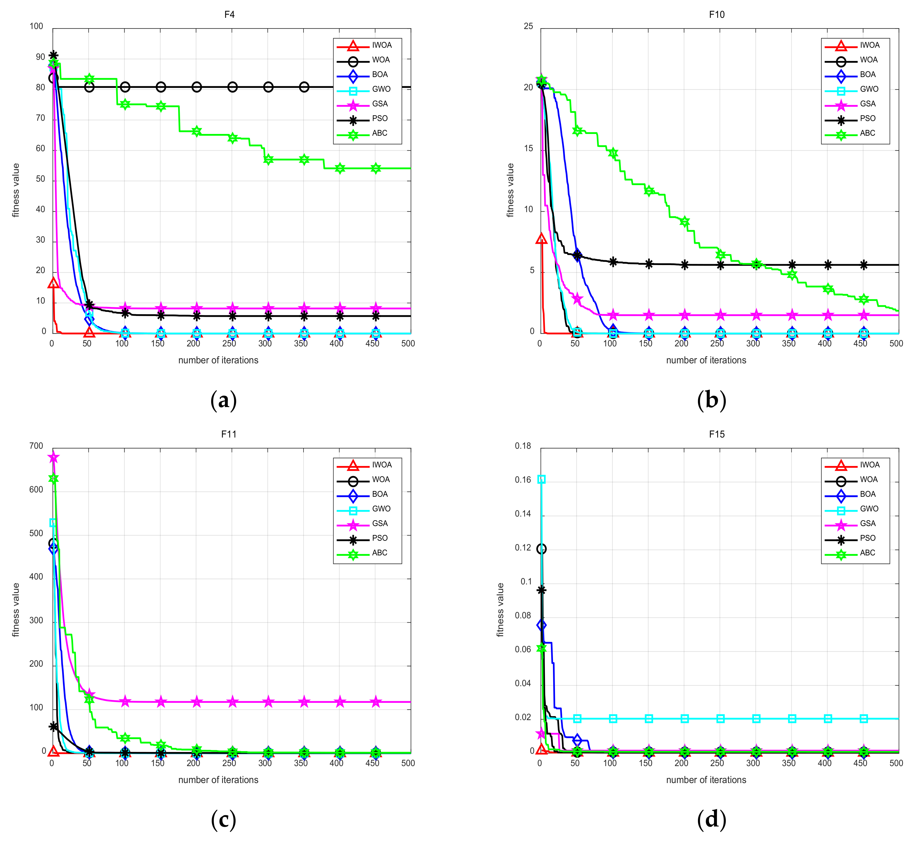
| Benchmark Function | Index | IWOA | WOA | GWO | BOA | GSA | PSO | ABC |
|---|---|---|---|---|---|---|---|---|
| F4 | mean | 5.43 × 10−159 | 43.92 | 8.92 × 10⁻⁷ | 6.10 × 10⁻⁹ | 10.32 | 6.39 | 51.84 |
| std | 2.33 × 10−158 | 26.61 | 1.13 × 10⁻⁶ | 4.32 × 10⁻¹⁰ | 2.55 | 1.89 | 4.95 | |
| F10 | mean | 8.88 × 10⁻¹⁶ | 3.84 × 10⁻¹⁵ | 1.01 × 10⁻¹³ | 5.93 × 10⁻⁹ | 0.31 | 5.68 | 2.03 |
| std | 0 | 2.60 × 10⁻¹⁵ | 1.63 × 10⁻¹⁴ | 5.42 × 10⁻¹⁰ | 0.55 | 1.02 | 0.57 | |
| F11 | mean | 0 | 9.704 × 10⁻³ | 5.10 × 10⁻³ | 4.92 × 10⁻¹² | 103.74 | 0.42 | 1.00 |
| std | 0 | 0.0370 | 9.1 × 10⁻³ | 2.77 × 10⁻¹² | 12.61 | 0.12 | 0.04 | |
| F15 | mean | 4.10 × 10⁻⁴ | 1.18 × 10⁻³ | 3.09 × 10⁻³ | 4.2198 × 10⁻⁴ | 0.01 | 5.08 × 10⁻⁴ | 6.97 × 10⁻⁴ |
| std | 9.73 × 10⁻⁵ | 1.8 × 10⁻³ | 6.8 × 10⁻³ | 2.00 × 10⁻⁴ | 5.8 × 10⁻³ | 3.49 × 10⁻⁴ | 7.23 × 10⁻⁵ |
| Inner Diameter/inch | Outer Diameter/inch | Sphere Diameter/inch | Pitch Diameter/inch | Number of Balls | Contact Angle |
|---|---|---|---|---|---|
| 0.9843 | 2.0472 | 0.3126 | 1.537 | 9 | 0° |
| Inner Diameter/mm | Outer Diameter/mm | Sphere Diameter/mm | Pitch Diameter/mm | Number of Balls | Contact Angle |
|---|---|---|---|---|---|
| 29.30 | 39.80 | 7.92 | 34.55 | 8 | 0° |
| WOA | SHO | GWO | BOA | AO | PSO | Ours | |
|---|---|---|---|---|---|---|---|
| a | 0.32804 | 0.26399 | 0.30998 | 0.25601 | 0.40434 | 0.24627 | 0.32974 |
| y1 | 1 | 0.93778 | 1 | 0.92205 | 1 | 0.99601 | 0.79091 |
| y2 | 5.5821 | 6.4616 | 5.5813 | 7.0254 | 5.4612 | 5.5798 | 6.0012 |
| b | 104.1000 | 46.8672 | 87.8477 | 39.3135 | 199.2539 | 44.0641 | 98.3366 |
| h | 0.1783 | 0.2363 | 0.1887 | 0.2478 | 0.1447 | 0.2385 | 0.2243 |
| Runtime | 5.091 s | 4.987 s | 5.294 s | 4.140 s | 6.751 s | 4.833 s | 4.860 s |
| SNR | −20.5843 | −20.652 | −20.5843 | −20.6751 | −20.5882 | −20.5883 | −20.5727 |
| WOA | SHO | GWO | BOA | AO | PSO | Ours | |
|---|---|---|---|---|---|---|---|
| a | 0.31153 | 0.2589 | 0.2082 | 0.28193 | 0.42522 | 0.25531 | 0.1871 |
| y1 | 0.97577 | 0.90102 | 1 | 0.95627 | 1 | 0.99815 | 0.64831 |
| y2 | 5.1517 | 6.3812 | 4.8249 | 5.092 | 4.8439 | 4.864 | 0.20993 |
| b | 2.9049 | 1.3462 | 1.3462 | 2.1783 | 7.8571 | 1.6936 | 1.3462 |
| h | 0.1894 | 0.2468 | 0.2468 | 0.2135 | 0.1354 | 0.2259 | 0.2468 |
| Runtime | 8.593 s | 4.100 s | 8.917 s | 14.060 s | 14.849 s | 10.825 s | 9.7066 s |
| SNR | −21.1669 | −21.2284 | −21.1558 | −21.1879 | −21.1562 | −21.1569 | −21.1289 |
Publisher’s Note: MDPI stays neutral with regard to jurisdictional claims in published maps and institutional affiliations. |
© 2022 by the authors. Licensee MDPI, Basel, Switzerland. This article is an open access article distributed under the terms and conditions of the Creative Commons Attribution (CC BY) license (https://creativecommons.org/licenses/by/4.0/).
Share and Cite
Huang, W.; Zhang, G.; Jiao, S.; Wang, J. Bearing Fault Diagnosis Based on Stochastic Resonance and Improved Whale Optimization Algorithm. Electronics 2022, 11, 2185. https://doi.org/10.3390/electronics11142185
Huang W, Zhang G, Jiao S, Wang J. Bearing Fault Diagnosis Based on Stochastic Resonance and Improved Whale Optimization Algorithm. Electronics. 2022; 11(14):2185. https://doi.org/10.3390/electronics11142185
Chicago/Turabian StyleHuang, Weichao, Ganggang Zhang, Shangbin Jiao, and Jing Wang. 2022. "Bearing Fault Diagnosis Based on Stochastic Resonance and Improved Whale Optimization Algorithm" Electronics 11, no. 14: 2185. https://doi.org/10.3390/electronics11142185
APA StyleHuang, W., Zhang, G., Jiao, S., & Wang, J. (2022). Bearing Fault Diagnosis Based on Stochastic Resonance and Improved Whale Optimization Algorithm. Electronics, 11(14), 2185. https://doi.org/10.3390/electronics11142185