A Big Data Approach for Demand Response Management in Smart Grid Using the Prophet Model

Abstract

Smart Grids (SG) generate extensive data sets regarding the system variables, viz., and demand and supply. These extremely large data sets are known as big data. Hence, preprocessing of this vast data and integration become critical steps in the load forecasting process. The precise prediction of the load is the primary concern while balancing the demand and supply in SG. Many techniques were devised for load forecasting using machine learning methods such as Deep-learning Models. However, in the case of large data sets, only a few models provide good performance, viz. Autoregressive Integrated Moving Average (ARIMA). However, this approach is complex, as it takes a minimum of 50 observations to make an evaluation. In this paper, the Prophet technique is used in the prediction of future demand response based on the past data, which is in the form of a time series. This technique is valid even if a few values in the time series are not available. Furthermore, the procedure is not affected by fluctuations, trends, and abnormal variations. The automatic model fitting approach is adopted for its effective performance. Further, ARIMA and Prophet model have been used to forecast and the approach is verified using various evaluation metrics. The demand response management was achieved and is being validated with two data sets. The results show the effectiveness of the Prophet model in the demand response management scheme involving large data sets.

1. Introduction

A smart grid differs from a traditional electricity system, which involves the flow of energy in one way. It enables real time collection of data in the transmission and distribution network facilitating monitoring of electricity for efficient energy management. It involves technologies such as data acquisition, control, automation, and communication, which work together in the grid to respond to the ever-changing demands of consumers. The flexibility can be achieved by making the customers follow demand response programs. However, several challenges are involved in implementing these programs in a real-time environment. Demand side management (DSM) in electrical power systems is one of the solutions to these challenges by shifting the flexibility of the power system to the consumer side.

Besides load forecasting, there are two kinds of demand response (DR) in the power sector: non-dispatchable and dispatchable demand response. A dispatchable demand response deals with the customer appliances. In some cases, the utility directs the consumer regarding cutting down the air conditioner or heater load during peak demand periods, thereby reducing the cost. Hence, the consumer will be directed only when the utility can forecast and predict the peak load. The problem arises when the forecasting model shows errors. The non-dispatchable demand response or the retail price-responsive demand is when the customer has the liberty to decide whether to cut down his consumption. It is based on the retail rate design and does not remain fixed. This includes dynamic pricing programs. In this case, the issue is redundant, and in most cases, the increase in prices has no perceptible effect on the consumption pattern of consumers. A vast amount of data is derived from the SG setup, on a second-by-second basis. However, there are various challenges associated with load forecasting using this data. First, the data, which is mostly accumulated, is unstructured, as it is gathered from a wide area containing a number of households. Second, the data collected is interlinked. Therefore, extraction of a particular data is found difficult for real-time applications. Many works have been carried out on load forecasting and demand response management using big data to solve these issues.

For managing the demand-response of energy, the authors have discussed the ARIMA model [1]. This model has the capability to lag its forecast errors by itself. It captures the consumed energy in the grid. In this paper, the ARIMA model is used to detect abnormalities. The authors have used automated fitting methods. However, it is not suitable for electricity consumption where there is a high variation in consumption behavior. Subsequently, the occupancy levels, which can improve the energy prediction, are highlighted. Their accumulated data is related to the premises of a residence [2]. Here, the authors collected data on the network activity and the consumption data of the consumers, on a daily basis. They used the ARIMA model to forecast with accuracy. It is acknowledged that the measurements of the constructed residence have a remarkable explanatory variable. In a similar work, the authors elaborated on a short to medium term load prediction model [3]. This paper highlighted the big data approach for smart homes.

The authors used big data in Ref. [4] for energy prediction. In a similar work [5], a data management system was used for forecasting. This model can help the customers to manage energy and reduce grid failure. They developed a model to make it economical and effective for better load distribution. In Ref. [6], the authors evaluated an hourly demand profile, which is effectively trained. Here, they used a hybrid model of the Bi-directional Long-Short-Term Memory (BLSTM) and the ARIMA model for the prediction of energy. In another work, the ARIMA model is used in all the phases of time series data. In a different work, Wang et al. dealt with short-term wind power prediction [7], where the ARIMA model was used for better performance [8]. Here, the authors described issues with a real-time price forecasting method. In Ref. [9], the authors randomized a consumer algorithm for managing demand response [10]. Moreover, the authors have designed an optimized demand response for efficient management of supply and demand in SG.

1.1. Related Work

Energy management is the most crucial part of an SG. For managing the supply and demand of energy, various big data analytics approaches were performed well in SG. Safhi et al. discussed load forecasting, which is based on big data [11]. There are various prediction techniques discussed in the literature for managing demand and supply gaps. The ARIMA model is an essential analytical method where time-series data is used. This model is trained to understand the data set in an efficient way. The ARIMA model has a great role in the prediction of the future trends of a time series. Krishna et al. discussed the ARIMA model, where it captures the process of energy consumption in the power system [1]. Moreover, it has the capability to check the validity of the consumed energy of the system.

The above model was unable to capture the experiment-based characteristics in a proper way. In order to overcome this limitation, the prophet model was proposed by some authors. In the work carried out by Ref. [12], the authors have used K-means clustering with the ARIMA model to obtain DR from an area in their university. They have used the data of two academic years viz., 2014–2015. First, they obtained the predicted electricity consumption data for 2016. The electricity consumption forecast was done, and DSM variables were obtained thereafter. In Ref. [13], the authors used two datasets viz., one dataset comprised the electricity consumption of three months (February–April 2013) and the other related to four years (July 2009–June 2013). In both of these datasets, the dynamic demand response was carried out using six different prediction models including ARIMA model and the results were finally compared.

The authors in Ref. [14] carried out work on applications of technologies involving big data, such as online monitoring of renewable energy systems and wind turbines, based on ultra-sphere model. The third application was backup and recovery in the electric power generation process. The authors believed that big data technologies are essential for buildings and handling SG. However, their research lacked the use of the big data in SG. In Ref. [15], the authors deal with the analysis of big data for renewable energy resources. They further aim at presenting techniques for Demand Response Management (DRM) using big data. The technology used to carry out the DRM is a simulator. While issuing DR, the simulator studies the big data and identifies correlations. The paper aims to use the technology and defined its usefulness in the future. However, the research was not made using different machine-learning techniques for carrying out the DR. By optimizing the programming, it would become easier for advancing the technology, in the near future.

The research in Ref. [16] was carried out to solve two main issues while handling big data. First, the authors used the expansion K-SVD sparse representation technique to extract hidden patterns of electricity consumption. Second, it can also be used to compress the data and store it efficiently. Further, they used a series of other computational techniques like SVM, PCA, etc., to classify the consumers into various groups. So, basically, they worked on efficient compression of data and its extraction. However, their research lacked obtaining a DR from the extracted data. In Ref. [17], the authors used big data technology to recognize the patterns of electricity consumption by consumers. They further shifted the peak load by studying the consumption patterns. They used the K-means algorithm to achieve the final clusters. However, they did not predict the future energy consumption patterns of the consumers.

The work in Ref. [18] was based on obtaining DR on electricity consumption data of one month only. The authors used big data technologies like Apache Spark to analyze the data to obtain DR and thereby successfully curtailed the air conditioner and heating loads. In Ref. [19], the authors created various priority lists varying from consumer to consumer. They further analyzed various aspects such as time, need, and power consumed while creating the priority lists. However, they did not do DSM using the priority lists. Furthermore, they did not predict the future electricity consumption by the consumers.

Almajarouee et al. introduced techniques based on peak load where the long-term forecasting provided results accurately. They tried to save cost and time by using this model [20]. Many authors discussed the Prophet model approach for the energy demand forecasting in SG. They tried to improve energy generation and consumption with accurate forecasting methods. In another paper, the authors discussed the data cleaning algorithm [21]. Here, the authors highlighted the errors in the models and various issues such as Benchmark-related algorithms. In a different work, the authors defined the smart energy management, which can maintain the quality of life for the consumer [22]. In this paper, the authors paid attention to minimizing the energy by developing an efficient model.

The energy consumption was managed [23] by using operational approach techniques. This technology is designed for proper communication with SG. The Energy Management System (EMS) has a significant role in managing demand and supply [24]. However, the studied data samples were small datasets. In another paper, the authors highlighted multiple homes. The problem formulation is carried out via multiple-knapsack problems [25]. In this paper, the authors discussed the importance of the external variables of consumed energy. They defined the state-of-the-art energy load forecasting method. They also defined the challenges that are involved with big data.

Table 1. Works related to energy forecasting for demand response.

S.No.	Author(s), Year	Techniques	Description	Application/Domain	Reference
1.	Newsham et al. (2010)	ARIMA model	To collect data related to the total occupied building, they installed wireless sensors in the building in the eastern zone in Ontario	Energy forecasting	[2]
2.	Krishna et al. (2015)	ARIMA model forecasting method	They used automatic model fitting methods	Energy prediction	[1]
3.	Asaleye et al. (2017)	Decision support tool	Used for renewable energy microgrids (DSTREM)	To ascertain daily energy consumption	[6]
4.	Luo et al. (2018)	An innovative hybrid RTP forecasting model	An RTP model was used for analyzing customer conducts. They got more benefit by scheduling the use of home appliances	Real-$\tilde{\mathrm{t}}$ime forecasting	[9]
5.	Sendric et al. (2019)	Data cleaning algorithm	To solve problems of ambiguous data from big data wireless sensor networks. They used these to clean data in smart cities	Cleaning ambiguous data	[21]
6.	Gupta et al. (2019)	Short-term wind power prediction (WPP) to improve the efficiency of power systems	Hybrid ARIMA-GARCH model	Forecasting of wind power	[8]
7.	Liu et al. (2020)	Big data analytics	Big data analytics in running smart cities	To build smart cities	[4]
8.	Wang et al. (2020)	Hybrid model based on the ARIMA model In this paper, Bi-directonal (Bi-LSTM) model and Bayesian optimization (BO) model	The ARIMA model can tackle the linear part of the time series data. Bi-LSTM can handle the non-linear features. The hybrid model provided a good prediction tool	The installation or replacement of electrolytic capacitors	[7]
9.	Almazrouee et al. (2020)	Prophet model	Prophet model used and forecasting accuracy compared with the Holt–Winter’s model.	To predict long-term peak loads	[20]

shows, at a glance, the various research work done in this area.

1.2. Motivation

ARIMA is mainly used by professionals who have prior knowledge of the intricacies of the model. If a single parameter in the equation is incorrect, the entire result will be affected. However, the Prophet model uses a Bayesian curve fitting method and does not require prior knowledge of datasets. It automatically finds seasonal trends from the data. The Prophet model incorporates seasonal trends such as holidays and weekends, whereas the ARIMA model incorporates both seasonal and non-seasonal trends with time-series data. It provides great precision compared to any other method.

1.3. Contribution

The ARIMA model requires expert knowledge as a prerequisite to make use of it. In addition, it is not flexible in use and is non-automatic. The Prophet model overcomes all the aforesaid limitations and is a powerful tool for prediction. It gives precise results with non-seasonal trends and also incorporates non-linear trends with datasets. The contribution of the proposed work is as follows:

• Optimized parameters for the Prophet and ARIMA model is used for better performance;
• Applied preprocessing techniques to clean the data;
• The abnormal data is removed for the prediction of consumption of energy in forecasting;
• ARIMA and the Prophet model is compared and analyzed with different performance metrics.

1.4. Organization

In this paper, Section 2 defines the detailed description of the methodology and workflow of our proposed model. Section 3 describes the performance of the models along with evaluation parameters. Subsequently, Section 4 is devoted to the discussion of the dataset and the Prophet model. Finally, the conclusion of this work is stated in Section 5.

2. Methodology

The methodology used for our current work is described in Figure 1. Initially, a high volume of data is obtained from the Smart Grid (SG) and the smart meters, which are connected to the electric power system. The dataset is a multivariate time-series data collected from Pennsylvania-New Jersey-Maryland Interconnection (PJM), which is a regional transmission organization (RTO) in the United States of America. PJM is a part of the Eastern Interconnection grid, operating an electric transmission system serving all parts of Delaware, Illinois, New Jersey, and North Carolina. The dataset is of the PJM East, which consists of data from 2014 to 2016 for the entire eastern region, where 2014 to 2015 is used for training and 2015 to 2016 is used for testing. The data consist of extraneous values and noises and hence the data needs to be filtered and the relevant data is extracted from the large datasets. Subsequent to processing, model fitting is done and then used in the Prophet model. The Prophet workflow model generates a reliable forecast in the form of time series values in the demand response process.

Further, in a traditional time series model, there are certain problems, as mentioned below.

• The time interval between data has to be the same throughout, while this is not a problem in Prophet model;
• Day with NA (nil data) is not allowed, while this is not an issue in the Prophet model;
• Seasonality with multiple periods is complex, while the Prophet model handles this problem by default;
• Parameter tuning by an expert is necessary for the ARIMA model, while in the Prophet model there is a default setting, from which parameters are easily interpreted. The Prophet model is extensively used in various fields for forecasting with an extensive range of data.

3. Mathematical Modeling of ARIMA and Prophet

3.1. Modeling of ARIMA

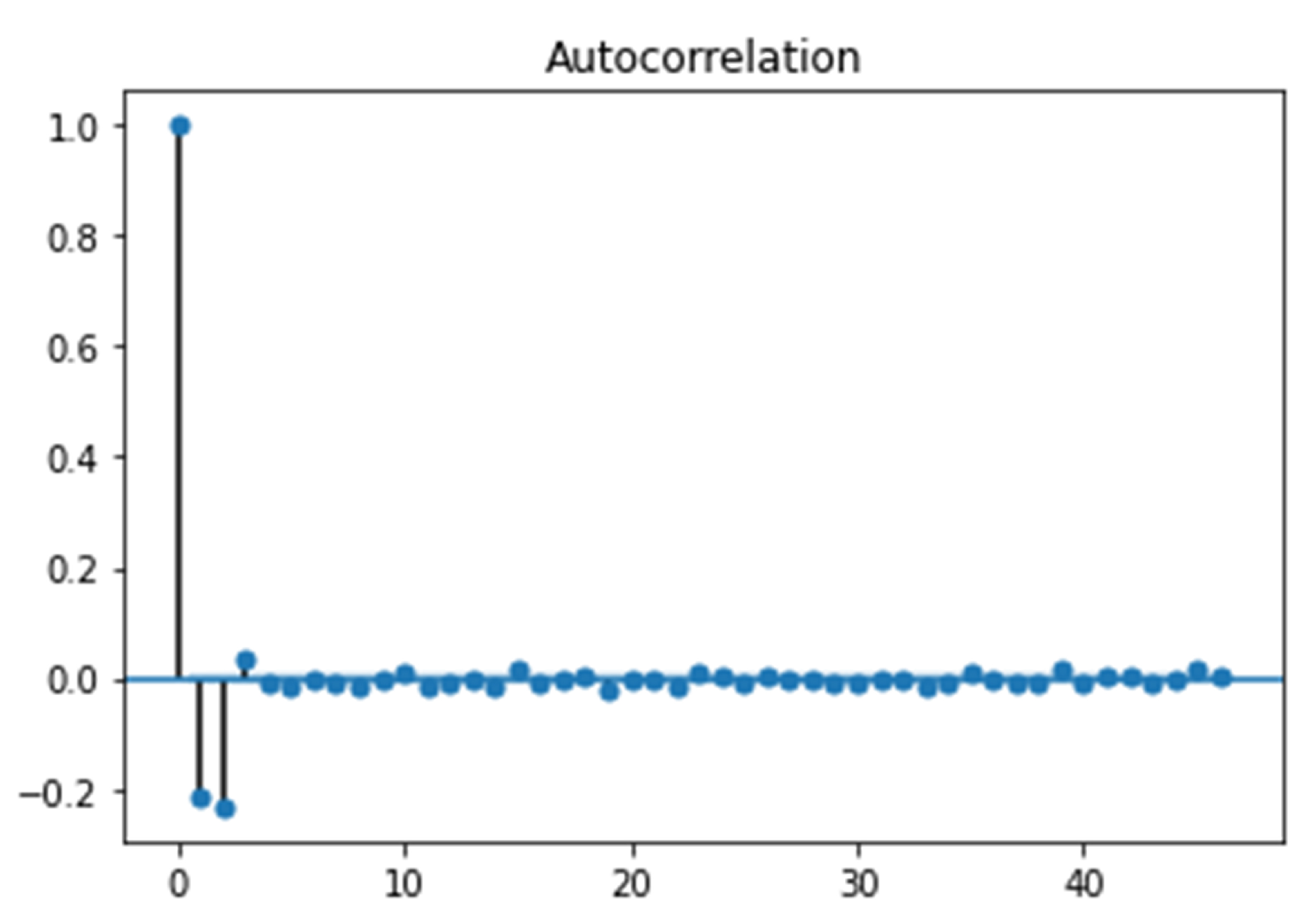
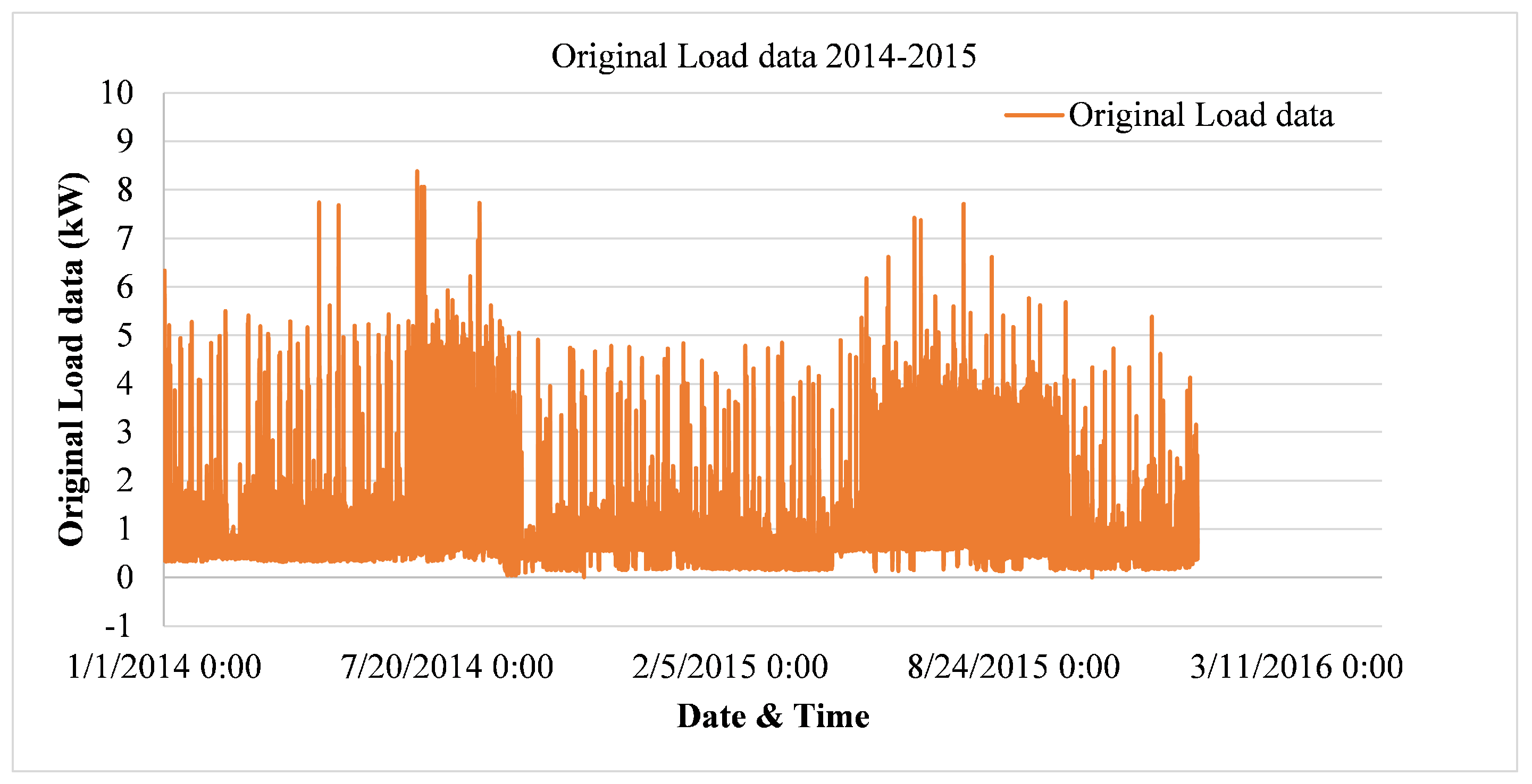
The ARIMA model processes data in a time series for making a prediction. The ARIMA model is used in both linear and multiple-regression models. The multiple regression model refers to the prediction of outcomes of dependent variables, which are based on variables of independent variables. The model is generally referred to as ARIMA (p, d, q), where p, d, and q are zero or positive numbers. The ARIMA model makes use of a stationary time series. Using a multiple linear regression model, it can work over non-stationary time series data. The values of p, q, and d can be found using auto-ARIMA. The process seeks to identify the most optimal parameters for the ARIMA model, settling on a single-fitted model. The process works by conducting differencing tests to determine the order of differencing ‘d’ and then fitting the models within the ranges of defined start p, max p, start q, and max q. The parameters p, q, and d were set to (4, 1, 1). Finally, the model trained on 2014–2015 data to obtain a prediction for 2016 consumption data.

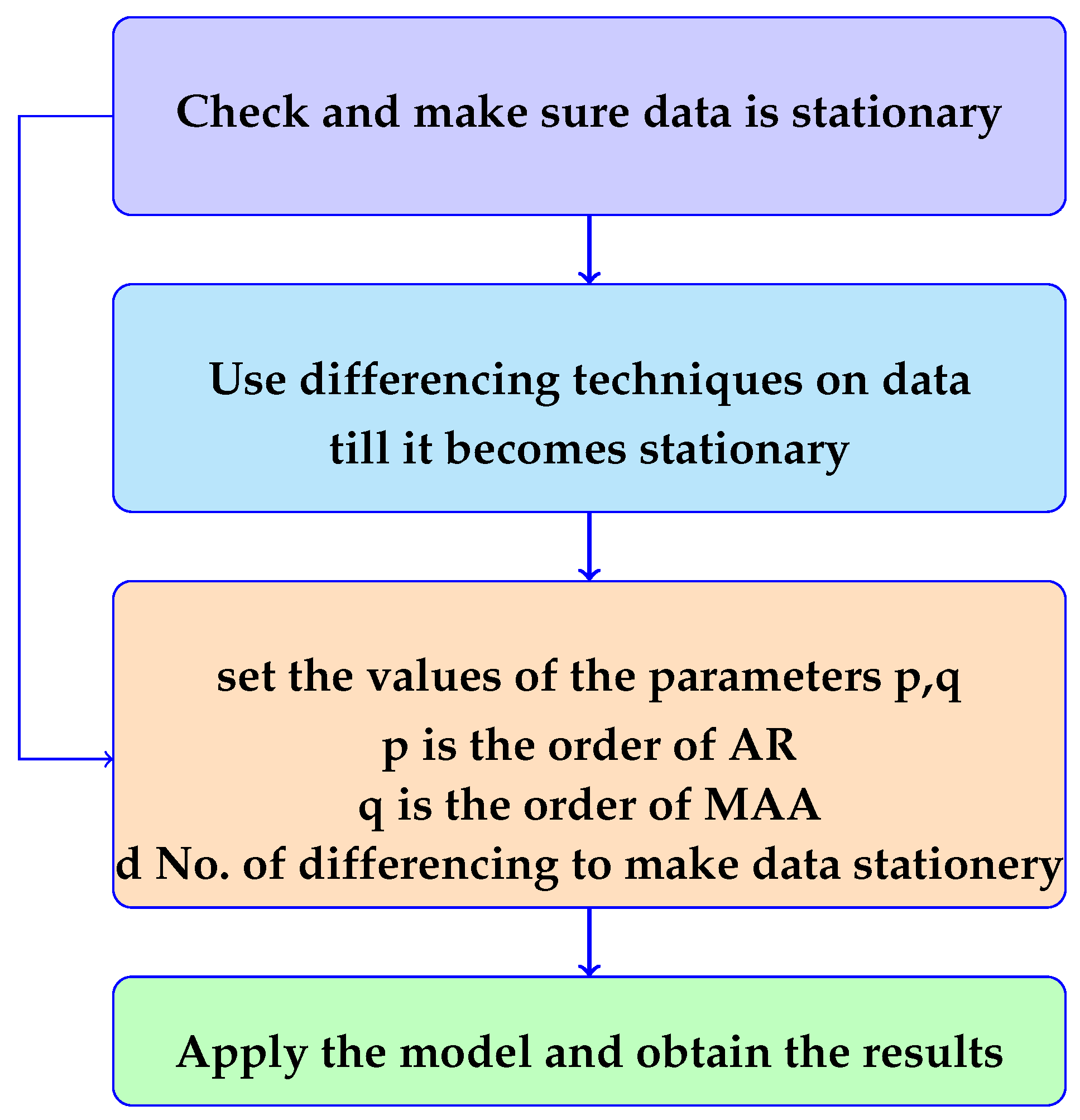
The ADF (Augmented Dickey Fuller) test is useful in detecting the unit root in a series to understand whether the series is stationary or non-stationary. Here, the null and alternate hypotheses state that if a series has a unit root, it fails to reject the null hypothesis, which says that the unit has a root. Then, the series is non-stationary. This means that the series can be linear, stationary, or difference stationary. The experimental results show that the ARMA (Auto Regressive Moving Average model) is based on real data, which is a stationary time series. In the flow chart shown in Figure 2, three features of the stationary data have been selected. Here, the first characteristic is the constant mean, the second one is the variance, which is also a constant, and the third characteristic is the co-variance, where the signal of past data, at different times, is constant.

Here, the daily stationary signal does not meet the first condition, but satisfies the second and third conditions. The moving average component of ARMA is set for change mean, and therefore, the first condition is not essential for the appropriate ARMA for a given time series. Later, the process of residual checking is completed.

If conditions are satisfied, then the process is stopped or otherwise continued. In Figure 2, the procedure of the ARIMA model is shown. Here, the power consumption datasets were collected and then the data is preprocessed. Subsequently, any abnormal data present in the datasets is eliminated. After the selection of features, the important features are extracted by using the classifier (Support Vectors Machine) and, at last, the predicted energy. On the basis of lagged data, future prediction is decided. In the above model, the equations are based on an autoregressive function. It is a function where the current value is generated based on the immediately preceding value. In the second process, the current value is generated based on the last two values. An AR (0) process would imply that there are no dependencies among the terms in the equations.

The aforementioned term predicts certain errors known as moving averages. The time series is differenced to make the data stationary. There are many models such as Randomwalk model, Random-trend model, Autoregressive model, and the Exponential-smoothing model. All are special cases of the ARIMA model. The time series representing the electricity consumption of a single consumer, at time t, is given by the value $Y_t$. The ARIMA model is discussed as in Figure 2 which represents the flow chart of the model where the parameters are indicated. Here, the values of parameters are selected and residual checking is done. The residual value is differenced between the observed value and the predicted value. The ARIMA model aims to predict power.

$$\begin{array}{c}\hfill Y_t=c+{\in }_t+\sum _{i=1}^q{\alpha }_i{X}_{t-i}+\sum _{k=1}^r{\beta }_k{\in }_{t-k}\end{array}$$

(1)

whereas $Y_t$ indicates the consumption of energy at time t, c indicates obstruction of the signal at q. $X_{t-i}$ and ${\alpha }_i$ are the parameters and regressors for the AR part of the model, respectively. It assumes Gaussian noise as in ${\in }_t$ and compounds q over time periods. Further, ${\in }_{t-k}$ and coefficient ${\beta }_k$ represent the parameters and regressors of the MA part of the model, respectively.

$$\begin{array}{c}\hfill f\left(x\right)=x^2+2x+1\end{array}$$

(2)

In Equation (2), $f\left(x\right)$ is the dependent variable and it indicates the prediction of the energy consumption using time series data. The values $x^2$ and $2x$ are independent variables and define the first-order differencing for making stationary data into a non-stationary data.

The prediction of the energy consumption in a time series data is described as follows:

$$\begin{array}{c}\hfill Z_{t1}={\alpha }_0-{\psi }_1(z_{t1}-1)-{\psi }_2(z_{t1}-2)-\cdots -{\psi }_z{n}_{t}1-p\\ \hfill +ϵ-{\alpha }_1({ϵ}_{t1}-1)-{\alpha }_2({ϵ}_{t_1}-2)-\cdots -\alpha ϵt1-q\end{array}$$

(3)

where at time $t_1$, $z_{t1}$ and ${ϵ}_{t1}$ are the predicted values and the random error of data $\psi (z_{t_1}-1)\cdots ,p$ indicates the model parameter, ${\alpha }_1\cdots q$ indicates the model parameter, p and q are represented by the autoregressive and moving average orders. Equation (3) shows some important cases of the ARIMA models, If $q_2$ = 0, then Equation (3) becomes an AR model of order $p_2$, and when $p_2=0$, the model decreases to a MA model to work with order $q_2$. The past data is the main basis in the prediction of energy by ARIMA model.

The general forecasting equation is:

$$\begin{array}{c}\hfill z_t=\mu +\varphi 1(z_t-1)+\dots +\varphi p{z}_t-p\\ \hfill -\theta 1(e_t-1)-\dots -\theta q{e}_t-q\end{array}$$

(4)

George Box and Gwilym Jenkins have introduced the moving average parameters $\left(\theta \right)$ having negative values in the equation. Hence, the actual numbers are used in the equation and there is no ambiguity, as the output was read by us at the time of using this software. These parameters are denoted by AR(1), AR(2)…AR(N), and MA(1), MA(2)…MA(N). To recognize a suitable ARIMA model for $Z_1$, the order of differencing viz., $\left(d_2\right)$ is to be decided. It is very important to make the series spatial so that the characteristics of seasonality can be removed. If the prediction of the differenced next series is constant, then we have to apply random-trend model. Here, the series is autocorrelated and the errors show the number of AR terms $(p_2\ge 1)$ and number MA $(q_2\ge 1)$. These are also needed in the equation. To determine the values of $p_2$, $d_2$ and $q_2$ is the best way for a given time series.

There are many types of non-seasonal ARIMA models that are discussed as follows: The ARIMA (1, 0, 0) model is denoted as the first-order autoregressive model. If the series is stationary and autocorrelated, then it can be forecast as a multiple of its own previous value, plus a constant. The forecasting equation, in this case is as below.

$$\begin{array}{c}\hfill Z_t=\mu +{\varphi }_1{Z}_{1t}-1\end{array}$$

(5)

In Equation (5), $Z_1$ is less developed data on itself by one period. This is an ARIMA (1, 0, 0) + constant model. If the mean value of $Z_1$ is zero, then the constant value will not be sufficient. If the slope coefficient $\varphi$ is positive and less than 1, $Z_1$ is stationary. If the value of the next time period value is predicted to be $\varphi$ times it creates a great distance from the mean, as this is a time value. If ${\varphi }_1$ is negative, it predicts a mean level with alteration of the signs. It also predicts that $Z_1$ will be below the mean of the next period if it is above the mean at that time.

In a second order autoregressive model ARIMA (2, 0, 0), there is $Y(t-2)$ term on the right, as well as on the left and depending on the signs and magnitudes of the coefficients. It describes a system where the mean level is of a sinusoidal wave pattern. It is like the motion of a mass on a spring that is subjected to random shocks. If the autoregressive coefficient is equal to 1, it is a series with an infinitely slow mean, which returns to the previous state. The equation for this model can be written as follows:

$$z_t-Z_{1}t-1=\mu$$

(6)

or equivalently

$$z_t=\mu +Z_{1}t+1$$

(7)

where the constant term is the mean, which periodically changes (i.e., the long-term drift) $Z_1$. This model could be fitted as a no-intercept regression model in which the first differencing of y is the dependent variable, as it includes only a nonseasonal difference and a constant term. It is “ARIMA0,1,0 with a constant.” The Random-walk without drift model would be ARIMA (0,1,0) without any constant. ARIMA1,1,0 is used as differenced with first-order in the autoregressive model. Here, autocorrelated means that the errors are found as in the Random walk model. Then the problem can be settled by adding past data of the dependent variable to the forecast equations, i.e., by regressing the first difference of z on itself lagged by one period. The forecast equation is:

$$\begin{array}{cc}\hfill Z_t-(Z_{1}t-1)& =\mu +{\varphi }_1(Z_{1}t-1)-(Z_{1}t-2)\hfill \end{array}$$

(8)

$$\begin{array}{cc}\hfill yt-(Z_{1}t-1)& =\mu \hspace{1em}\hspace{1em}\hspace{1em}\hspace{1em}\hspace{1em}\hspace{1em}\hspace{1em}\hspace{1em}\hspace{1em}\hspace{1em}\hfill \end{array}$$

(9)

3.2. The Modeling of Prophet

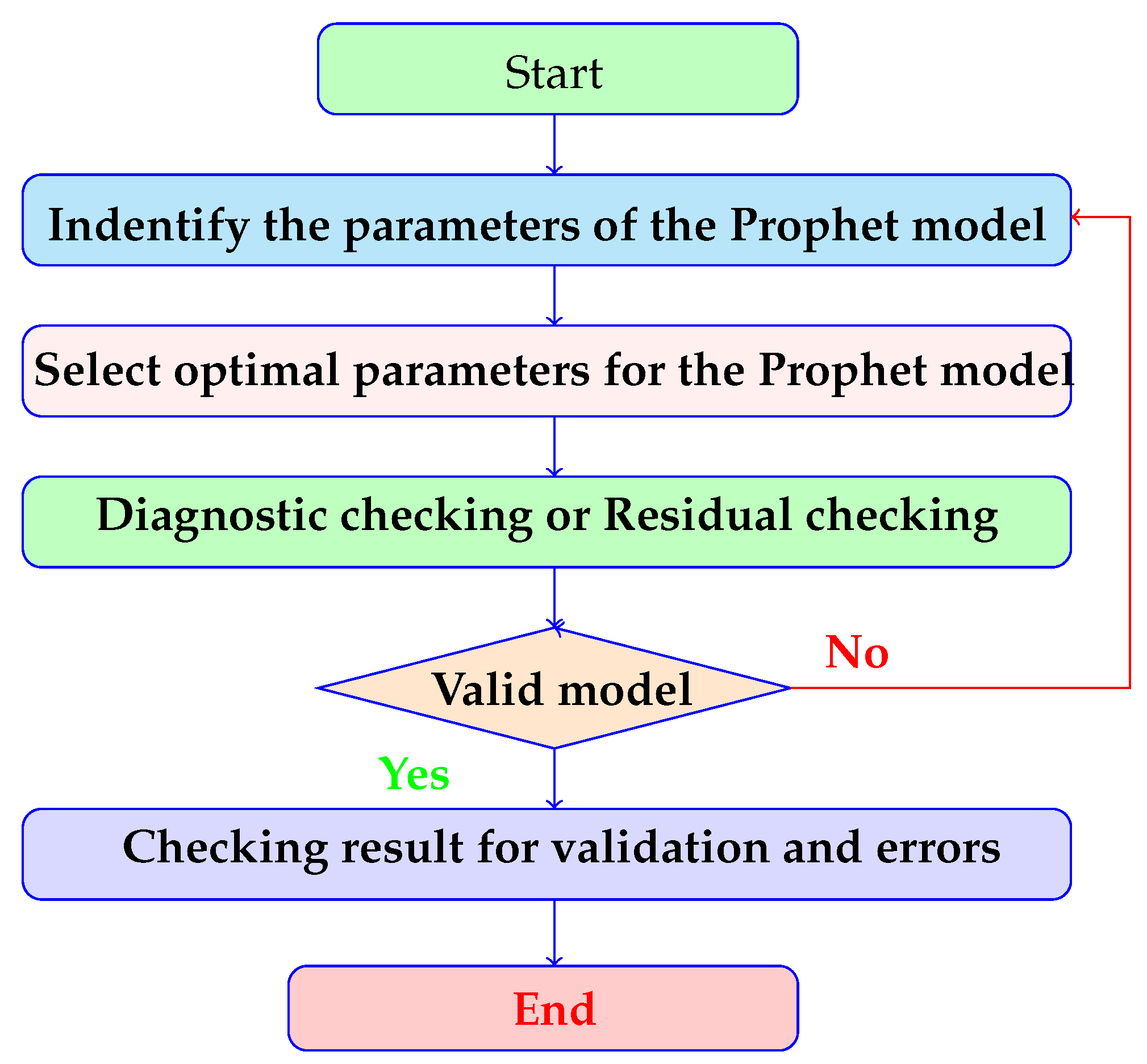
Prophet has been developed by Facebook in order to overcome some problems that exist in ARIMA. Prophet works through the use of an additive model whereby the non-linear trends in the series are fitted with the appropriate seasonality. It is a time series predictive method where the aim is to predict power in SG. The flow chart of Prophet model is shown in Figure 3. For this purpose, appliances are categorized as: interruptible, non-interruptible, and base appliances. Power categorization of:

• Interruptible Appliances

  $$\begin{array}{c}\hfill F_{in}=\sum _{t-1}^U\sum _{ineIN}{\sigma }_{in}\ast r{w}_{in}\left(t\right)\end{array}$$

  (10)

  where $F_{in}$ is the power consumption of appliances, $ineIN$ indicates Interruptible Appliance, ${\sigma }_{in}$ indicates power rating, U is the total time slot, and $r{w}_{in}\left(t\right)$ is the state of each Interruptible Appliance at time slot t.

  $$r{w}_{in}\left(t\right)=\sum \left\{\begin{array}{cc}0\hfill & \mathrm{if}\mathrm{appliances}\mathrm{are}\mathrm{off}\hfill \\ 1\hfill & \mathrm{if}\mathrm{appliances}\mathrm{are}\mathrm{on}\hfill \end{array}\right.$$

  (11)
• Non-interruptible Appliances

  $$F_{in}=\sum _{t-1}^U\sum _{niNI}{\sigma }_{n}i\ast r{w}_{in}\left(t\right)$$

  (12)

  where $F_{in}$ is the power consumption of appliances, $niNI$ indicates Non-Interruptible Appliance, ${\sigma }_{in}$ indicates power rating, U is total time slot, and $r{w}_{in}\left(t\right)$ is the state of each Non-Interruptible Appliances at time slot t.

  $$r{w}_{in}\left(t\right)=\sum \left\{\begin{array}{cc}0\hfill & \mathrm{if}\mathrm{appliances}\mathrm{are}\mathrm{off}\hfill \\ 1\hfill & \mathrm{if}\mathrm{appliances}\mathrm{are}\mathrm{on}\hfill \end{array}\right.$$

  (13)
• Base appliances are similar to fixed appliances that do not have flexibility of operation. The pattern of consumption of energy and operational period of appliances cannot be changed. It is important that these appliances must be ‘ON’ when the user wants to switch them ON such as home appliances viz. TV, fridge, and other devices.

  $$F_b=\sum _{t-1}^U\sum _{beB}{\sigma }_B\ast r{w}_B\left(t\right)$$

  (14)

  where $F_b$ represents total energy consumption, B is the base appliance at time t, $r{w}_B$ is each base appliance, and ${\sigma }_B$ is the power rating.

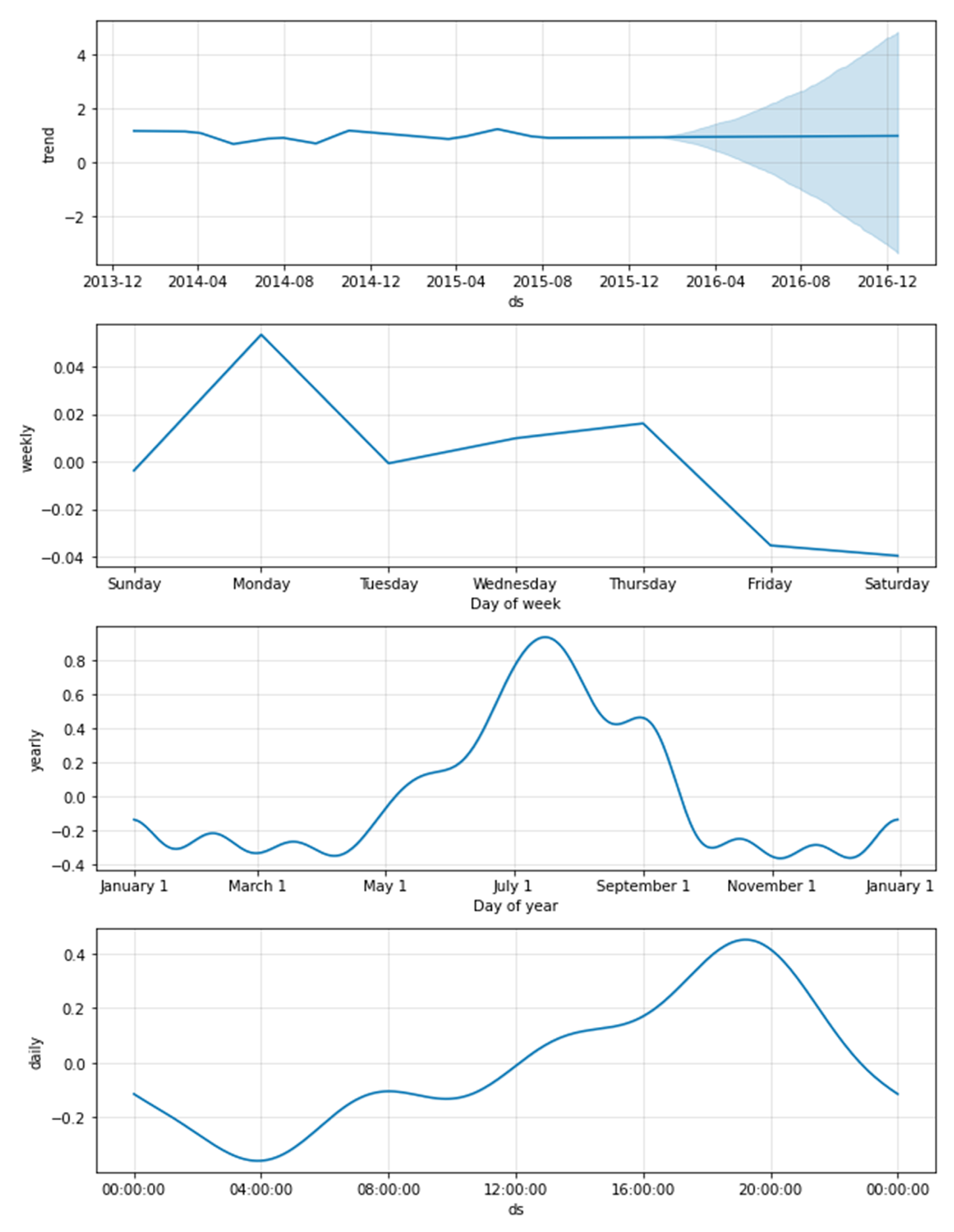
Since the Prophet model works on data trends, holidays and seasonal data provides complex features. Seasonality is input on the basis of day, week, and year. The prophet model, where consumption is represented by time series, is a data method expressed as follows,

$$\begin{array}{c}\hfill Z\left(t\right)=Y\left(t\right)+S\left(t\right)+H\left(t\right)+E\left(t\right)\end{array}$$

(15)

where $Z\left(t\right)$ indicates the consumption, $Y\left(t\right)$ represents the data trend function, $S\left(t\right)$ indicates the seasonal data, $H\left(t\right)$ indicates the holiday-based data, and $E\left(t\right)$ represents the errors.

The trend function of the Prophet model $H\left(t\right)$ is highlighted by a piecewise linear growth model. It is also called a Saturation-growth model. The maximum load data does not show a saturating growth, which is a piecewise linear growth model represented as follows:

$$\begin{array}{c}\hfill h\left(t\right)=(l+a{\left(t\right)}^T\delta )t+(n+a{\left(t\right)}^T\sigma )\end{array}$$

(16)

Here l is the growth rate, $\delta$ indicates rate adjustment, n is an offset parameter, and $\sigma$ is the change point.

$$b_j\left(t\right)=\left\{\begin{array}{cc}1\hfill & \mathrm{if}t\ge U_k\hfill \\ 0\hfill & \mathrm{otherwise}\hfill \end{array}\right.$$

where $b_j$ is the output and $U_k$ is the change point.

The seasonality function is manifested by the following equation:

$$\begin{array}{c}\hfill T\left(t\right)=\sum _{n=1}^L(b_{n}cos(2\ast p\ast in\ast t/q)\\ \hfill +d_{n}sin(2\ast p\ast in\ast t/q)\end{array}$$

(17)

In Equation (17), $T\left(t\right)$ is the seasonality function. Here, the time series multiperiod seasonality method is used. The Fourier series is applied to the daily and seasonal changes. Therefore, the seasonality function is discussed as:

$$\begin{array}{c}\hfill A_t=[1(t\in E_1),\cdots ,1(t\in C_m)]\end{array}$$

(18)

Here, $A_t$ indicates the matrix of regresses, E indicates holidays, and 1 represents the holidays parameter.

$$\begin{array}{c}\hfill H_t=A\left(t\right)l\end{array}$$

(19)

In Equation (19), $H_t$ indicates holidays and l indicates a corresponding change in the forecast. It produces estimates of unknown variables.

4. Results and Discussion

4.1. Description of Datasets

This section provides the description of the datasets.

Table 2. Preference matrix for different devices.

S.No.	Time/Reason	Priority
1	00:01–03:00	Fridge	Air conditioner	Tubelight	Microwave oven	Sandwich Maker	Dishwasher	Hair dryer	Vacuum cleaner	Washing machine	Clothes dryer
	Reason	Fridge is essential for use 24 h a day. The other items are taken according to priorities during the course of the day
2	3:01–6:00	Fridge	Air conditioner	Tubelight	Dish washer	Microwave oven	Sandwich maker	Hair dryer	Vacuum cleaner	Washing machine	Clothes dryer
	Reason	The dishwasher is placed as the fourth priority here. Some people sleep early and wake up early.
3	6:01–9:00	Fridge	Tubelight	Dish washer	Hair dryer	Sandwich maker	Microwave oven	Washing machine	Vacuum cleaner	Clothes dryer	Air conditioner
	Reason	It is time to go to school and office in the morning.
4	9:01–12:00	Fridge	Washing machine	Vacuum cleaner	Clothes cryer	Microwave oven	Sandwich maker	Hair dryer	Dish washer	Air conditioner	Tubelight
	Reason	People leave home for office by 9:00 a.m. Thereafter, the priority for people at home is to clean the house and wash clothes.
5	12:01–15:00	Fridge	Clothes dryer	Air conditioner	Microwave oven	Dishwasher	Hair dryer	Vacuum cleaner	Washing machine	Tubelight	Sandwich maker
	Reason	It is lunchtime, so the microwave oven is used. Besides, the ambient temperature is high. So, the air conditioner is also used.
6	15:01–18:00	Fridge	Dish washer	Air conditioner	Tubelight	Microwave oven	Sandwich maker	Washing machine	Clothes dryer	Hair dryer	Vacuum cleaner
	Reason	It is time to take an afternoon nap and wake up for tea in the evening
7	18:01–21:00	Fridge	Tubelight	Microwave oven	Hair dryer	Air conditioner	Sandwich maker	Dishwasher	Vacuum cleaner	Washing machine	Clothes dryer
	Reason	Now, it is time for people to return from the office, take a bath, and use the hair dryer. After dinner they relax using the air conditioner.
8	21:01–24:00	Fridge	Tubelight	Air conditioner	Microwave oven	Dishwasher	Hair dryer	Sandwich maker	Vacuum cleaner	Washing machine	Clothes dryer
	Reason	Some people return late from the office, and usually have their dinner at 9:00 p.m.

shows the consumer preference regarding the appliance taken with the reason for selection. The dataset taken is hourly time series and forecasting was done using Facebook’s Prophet model and ARIMA model. The energy consumption has unique characteristics. First, the electricity consumption for the year 2016 was predicted using the ARIMA model. However, to make use of the ARIMA model, it must be made sure that the data is stationary.

A stationary time series data has its mean, variance, and other statistical properties constant over a given time frame. The data used here is shown in

Table 3. A sample of the Smart Grid dataset.

Date: 1 January 2014
Time	Energy kWh/Half-Hour
00:00.0	0.488
30:00.0	0.449
00:00.0	0.424
30:00.0	0.439
00:00.0	0.291
30:00.0	0.262
00:00.0	0.308
30:00.0	0.138
00:00.0	0.404

. It is a collection of data from the source [26]. The aforesaid data helps in the visualization and analysis of the changes. In addition, the future trend of the variables under analysis can be predicted using Machine-learning Algorithms. The entire dataset used is from smart meter energy user data from households. It had half-hour time stamps and generated energy data in kWh/half-hour. This data was comprised of 1 million values, from which our final dataset of 149,999 were extracted. The dataset used for analysis contained 100,000 values and the test dataset contained 49,999 values.

Table 4. Home appliances rating used in households.

S.No.	Name of the Appliance	Rating (KWh)
1	Fridge	0.2
2	Tubelight	0.055
3	Air conditioner	4
4	Microwave	1.7
5	Dishwasher	1.5
6	Hair dryer	1
7	Sandwich maker	1
8	Vacuum cleaner	1.4
9	Washing machine	0.5
10	Clothes dryer	2.5

shows the rating of each of the appliances. A sample of the final data set is shown in

Table 5. Consumption dataset from the households.

Date: 4 October 2016
Units of All the Columns Are in kW Except Column 2 in Wh and Column 3 in (Wh/hh)
Time	Energy	Wh/hh	Genneration	AC	Furnace	Cellar Lights	First Floor Lights	Dining Room	Microwave	Total Load
30:00	$8\times {10}^{-2}$	$4\times {10}^1$	$5.78\times {10}^{-5}$	$9.53\times {10}^{-3}$	$5.34\times {10}^{-3}$	$1.26\times {10}^{-4}$	$1.12\times {10}^{-2}$	$4.3\times {10}^{-3}$	$4.73\times {10}^{-1}$	$3.1\times {10}^1$
00:00	$1.09\times {10}^{-1}$	$5.45\times {10}^1$	$1.53\times {10}^{-3}$	$3.64\times {10}^{-1}$	$5.52\times {10}^{-3}$	$4.33\times {10}^{-5}$	$2.35\times {10}^{-2}$	$3.59\times {10}^{-3}$	$4.45\times {10}^{-3}$	$7.28\times {10}^{-1}$
30:00	$1.13\times {10}^{-1}$	$5.65\times {10}^1$	$1.85\times {10}^{-3}$	$4.18\times {10}^{-1}$	$5.50\times {10}^{-3}$	$74.44\times {10}^{-5}$	$2.3\times {10}^{-2}$	$3.52\times {10}^{-3}$	$4.40\times {10}^{-3}$	$6.26\times {10}^{-1}$
00:00	$4.1\times {10}^{-1}$	$2.05\times {10}^2$	$1.74\times {10}^{-3}$	$4.11\times {10}^{-1}$	$5.56\times {10}^{-3}$	$5.94\times {10}^{-5}$	$3.4\times {10}^{-3}$	$3.4\times {10}^{-3}$	$4.26\times {10}^{-3}$	$7.83\times {10}^{-1}$
30:00	$5.4\times {10}^{-2}$	$2.7\times {10}^1$	$3\times {10}^{-5}$	$1.72\times {10}^{-2}$	$5.3\times {10}^{-3}$	$1.19\times {10}^{-4}$	$2.39\times {10}^{-2}$	$3.92\times {10}^{-3}$	$4.41\times {10}^{-3}$	$1.99\times {10}^{-1}$
00:00	$4.30\times {10}^{-2}$	$2.15\times {10}^1$	$4.42\times {10}^{-4}$	$1.27\times {10}^{-1}$	$5.42\times {10}^{-3}$	$5.44\times {10}^{-5}$	$2.38\times {10}^{-2}$	$3.81\times {10}^{-3}$	$4.40\times {10}^{-3}$	$4.98\times {10}^{-1}$

. A total of 24 appliances were taken into consideration for the analysis.

4.2. Prediction Using the ARIMA Model

The combined dataset is shown in Figure 4, which consists of stationary time series data from 2014 to 2015. Further, Figure 5 depicts another data from 2014 to 2015. In the beginning, it was predicted based on the electric consumption for the year 2016 using the ARIMA model. Before applying the ARIMA model, it must be made sure that the data is stationary. With the graph plotted in Figure 4, it can be observed that the data is not in stationary mode. The difference between the present and the previous period gives us the first differencing value as shown in Figure 6 The obtained values are then plotted to check if the statistical properties are constant. If they are still not constant, the second differencing is obtained using the first differencing values.

Figure 6 depicts the data undertaken and the autocorrelation present in the datasets.

The method of differencing needs to be applied, repeatedly, till the data obtained becomes stationary. The checking of the correlation between the data with its past values is called autocorrelation. For this, the autocorrelation function plot (ACF) is used. The plot shows the correlation between various points. The correlation coefficient is plotted on the x-axis with the number of lags on the y-axis. The ACF plot is mainly used to determine which one among them is to be used as data.

When differencing is done, the data obtained generally oscillate. This means that the subject data has achieved the constant values of statistical variables.

That is, the data is now stationary and ready to be worked upon using the ARIMA model. Subsequent to making the data stationary, the parameters (p, q, d) are as follows:

• p: order of the AR term;
• q: order of the MA term, and;
• d: number of differencing required to make the time series stationary.

In Figure 7, the blue line represents the consumption data of the predicted values for the year 2016. After extensive computation, these three values were set to be (1,0,4). Finally, the model was trained on the data relating to the years 2014–2015 to obtain a prediction for 2016. The data can be considered as stationary if it has constant amplitude and oscillates in the given time frame. In the case of signal with noise, The ARIMA model acts as a filter to extract the data of the signal from the given system. The extracted signal is then worked upon to carry out future predictions. For fitting the data on the ARIMA model, it is important to make the data stationary using the differencing technique to obtain standardized data, as shown in Figure 8.

4.3. Prediction Using the Prophet Model

The electricity consumption data from 2014 to 2015 was used to work out with the help of the Facebook Prophet Model. The forecast for the data of 2016 was done using the model’s inbuilt predictions. Figure 5 depicts the data from 2014 to 2015. The model was trained on this data to predict the electricity data for a later year. Figure 9 summarizes all the computations carried out in the process. The predicted values are in quite good sync with the original data, and hence a forecast was made for the year 2016. There could be certain variations in the actual data of 2016, and a margin of the upper and the lower bound were created. Figure 9 indicates the trend of the predicted data. Figure 10 shows the trend exhibited by the predicted data for the electricity consumption for a year; the seasonality is considered.

The various components of the Prophet model included were weekly, yearly, and daily components and the trend exhibited by the predicted values. Figure 10 shows the predicted and actual values for 2016. The values predicted, as shown in

Table 6. Performance comparison of the ARIMA and Prophet model for different evaluation parameters.

Model	MSE	RMSE	MAE	MAPE
ARIMA	1.06877	1.03381	0.6239	1.1932
Prophet	0.67546	0.82186	0.5308	1.0399

with the original 2016 data are compared for both the ARIMA and the Prophet model. In case of the Prophet model, the mean square error is 0.67546 and the mean absolute error is 0.5308. The same is 1.06877 and 0.6239, respectively, for the ARIMA model. It is seen that the root mean square error and mean absolute percentage error of the Prophet model are significantly less than those of the ARIMA model. Hence, after comparing the two models, it has been found that the DR from the Prophet model has better overall performance.

Table 7. Optimized parameters for the ARIMA and Prophet model.

SN	Model	Parameters
1	ARIMA	P(A = 4), Q(Integration = 1), d(differences = 1)
2	Prophet	T(Trend = 1.4), S(seasonality = 4), H(holiday = 1)

shows the optimized parameters values of the ARIMA and Prophet models. The parameters are optimized through a random approach in which a random set is generated, training the model on the generated model, and finally making predictions. The set of parameters that gives the highest prediction accuracy is selected.

Facebook’s Prophet Model is selected for carrying out DSM in the subject research. The data was fed to the appliances at home and the appliances were switched off one-by-one on the basis of priority of usage. Figure 11 shows the DSM on the predicted values. The demand response was carried out between the total load and the generated electricity. For the DSM, the difference between the original and the predicted values of the year 2016 are calculated and presented, as shown in Figure 12. The trend, over different time lengths, shown in Figure 13, can be useful for controlling the electric consumption of the appliances in households.

5. Conclusions and Future Scope

The forecasting of demand and supply of electrical energy is essential and critical in achieving efficiency and economy in the running of an SG. The time-series data available for the purpose in a real-life situation is, at times, discontinuous. The same has to be the basis for a forecast in the absence of alternatives. The ARIMA model is seen to provide a good forecast if the data provided is complete. However, it is also very expensive, as its computation requires computer systems with memory and computational speeds of a very high order. The Prophet model, while offsetting all the above limitations of the ARIMA model, generates a reliable forecast even in the absence of a few values in the data. Therefore, the Prophet model is preferable compared to ARIMA in real time data.

In this paper, we used households datasets that consist of 10,00,000 records. Due to the large datasets, we used ARIMA and Prophet for higher accuracy and lower error rate. Further, due to the unavailability of the datasets of different years, the performance of the Prophet can not be checked. However, it may give better results in next year prediction. In future works, we need to explore more time series prediction models in real time. In addition, we need to explore optimization algorithms for tuning the parameters of the models.

References

1. Badrinath Krishna, V.; Iyer, R.; Sanders, W. ARIMA-Based Modeling and Validation of Consumption Readings in Power Grids. In Proceedings of the International Conference on Critical Information Infrastructures Security, Berlin, Germany, 5–7 October 2015; pp. 199–210. [Google Scholar] [CrossRef]
2. Newsham, G.; Birt, B. Building-level occupancy data to improve ARIMA-based electricity use forecasts. BuildSys’10. In Proceedings of the 2nd ACM Workshop on Embedded Sensing Systems for Energy-Efficiency in Buildings, Zurich, Switzerland, 2 November 2010. [Google Scholar] [CrossRef] [Green Version]
3. Chatterjee, S.; Dey, S.; Dasgupta, M. A Solution to Demand Response with Soft-Computing Techniques. In Proceedings of the 2020 Fourth International Conference on Inventive Systems and Control (ICISC), Coimbatore, India, 8–10 January 2020; pp. 122–126. [Google Scholar] [CrossRef]
4. Liu, H. Smart Cities: Big Data Prediction Methods and Applications; Springer: Singapore, 2020. [Google Scholar]
5. Viloria, A.; Prieto Pulido, R.; Guiliany, J.; Ventura, J.; Palma, H.; Torres, J.; Bilbao, O.; Lezama, O. Analyzing and Predicting Power Consumption Profiles Using Big Data. In Proceedings of the International Conference on Dependability in Sensor, Cloud, and Big Data Systems and Applications, Guangzhou, China, 12–15 November 2019; pp. 392–401. [Google Scholar] [CrossRef]
6. Asaleye, D.; Breen, M.; Murphy, M. A Decision Support Tool for Building Integrated Renewable Energy Microgrids Connected to a Smart Grid. Energies 2017, 10, 1765. [Google Scholar] [CrossRef] [Green Version]
7. Wang, Z.; Qu, J.; Fang, X.; Li, H.; Zhong, T.; Ren, H. Prediction of early stabilization time of electrolytic capacitor based on ARIMA-Bi_ LSTM hybrid model. Neurocomputing 2020, 403, 63–69. [Google Scholar] [CrossRef]
8. Gupta, A.; Sharma, K.; Vijayvargia, A.; Bhakar, R. Very Short term Wind Power Prediction Using Hybrid Univariate ARIMA-GARCH Model. In Proceedings of the 2019 8th International Conference on Power Systems (ICPS), Jaipur, India, 20–22 December 2019; pp. 1–6. [Google Scholar] [CrossRef]
9. Luo, X.; Zhu, X.; Lim, E. A hybrid model for short term real-time electricity price forecasting in smart grid. Big Data Anal. 2018, 3, 8. [Google Scholar] [CrossRef]
10. Pal, R.; Chelmis, C.; Frincu, M.; Prasanna, V. Towards Dynamic Demand Response on Efficient Consumer Grouping Algorithmics. IEEE Trans. Sustain. Comput. 2016, 1, 20–34. [Google Scholar] [CrossRef]
11. Safhi, H.M.; Frikh, B.; Ouhbi, B. Energy load forecasting in big data context. In Proceedings of the 2020 5th International Conference on Renewable Energies for Developing Countries (REDEC), Marrakech, Morocco, 29–30 June 2020; pp. 1–6. [Google Scholar] [CrossRef]
12. Nepal, B.; Yamaha, M.; Yokoe, A.; Yamaji, T. Electricity load forecasting using clustering and ARIMA model for energy management in buildings. Jpn. Archit. Rev. 2020, 3, 62–76. [Google Scholar] [CrossRef] [Green Version]
13. Aman, S.; Frincu, M.; Chelmis, C.; Noor, M.; Simmhan, Y.; Prasanna, V.K. Prediction Models for Dynamic Demand Response-Requirements, Challenges, and Insights. In Proceedings of the 2015 IEEE International Conference on Smart Grid Communications (SmartGridComm), Miami, FL, USA, 2–5 November 2015; pp. 338–343. [Google Scholar] [CrossRef]
14. Zhan, J.; Huang, J.; Niu, L.; Peng, X.; Deng, D.; Cheng, S. Study of the key technologies of electric power big data and its application prospects in smart grid. In Proceedings of the 2014 IEEE PES Asia-Pacific Power and Energy Engineering Conference (APPEEC), Hong Kong, China, 7–10 December 2014; pp. 1–4. [Google Scholar] [CrossRef]
15. Ku, T.Y.; Park, W.K.; Choi, H. Demand Response Operation Method on Energy Big Data Platform. In Proceedings of the 2018 Tenth International Conference on Ubiquitous and Future Networks (ICUFN), Prague, Czech Republic, 3–6 July 2018; pp. 823–825. [Google Scholar] [CrossRef]
16. Wang, Y.; Chen, Q.; Kang, C.; Xia, Q.; Luo, M. Sparse and Redundant Representation-Based Smart Meter Data Compression and Pattern Extraction. IEEE Trans. Power Syst. 2017, 32, 2142–2151. [Google Scholar] [CrossRef]
17. Zhang, X.; Li, D.; Cheng, M.; Zhang, P. Electricity consumption pattern recognition based on the big data technology to support the peak shifting potential analysis. In Proceedings of the 2014 IEEE PES Asia-Pacific Power and Energy Engineering Conference (APPEEC), Hong Kong, China, 7–10 December 2014; pp. 1–5. [Google Scholar] [CrossRef]
18. Vajjala, V.A.H. A novel solution to use Big Data technologies and improve demand response program in aggregated residential houses. In Proceedings of the 2016 IEEE Conference on Technologies for Sustainability (SusTech), Phoenix, AZ, USA, 9–11 October 2016; pp. 251–256. [Google Scholar] [CrossRef]
19. Singh, S.; Yassine, A. Mining Energy Consumption Behavior Patterns for Households in Smart Grid. IEEE Trans. Emerg. Top. Comput. 2019, 7, 404–419. [Google Scholar] [CrossRef]
20. Almazrouee, A.; Almeshal, A.; Almutairi, A.; Alenezi, M.; Alhajeri, S. Long-Term Forecasting of Electrical Loads in Kuwait Using Prophet and Holt-Winters Models. Appl. Sci. 2020, 10, 5627. [Google Scholar] [CrossRef]
21. Sandrić, B.; Marcelić, M.; Topolovac, I.; Jurčevic, M. Survey of data cleaning algorithms in wireless sensor networks. In Proceedings of the 2019 2nd International Colloquium on Smart Grid Metrology (SMAGRIMET), Split, Croatia, 9–12 April 2019; pp. 1–4. [Google Scholar] [CrossRef]
22. Hrnjica, B.; Mehr, A.D. Energy Demand Forecasting Using Deep Learning. In Smart Cities Performability, Cognition, & Security; Al-Turjman, F., Ed.; Springer: Cham, Switzerland, 2020; pp. 71–104. [Google Scholar] [CrossRef]
23. Grigoraş, G.; Cârţină, G.; Bobric, E.C. Trends and Directions for Energy Saving in Electric Networks. In Management of Technological Innovation in Developing and Developed Countries; Sun, H., Ed.; IntechOpen: Rijeka, Croatia, 2012; Chapter 1. [Google Scholar] [CrossRef] [Green Version]
24. Forbes, J.W., Jr. System, Method, and Apparatus for Electric Power Grid and Network Management of Grid Elements. U.S. Patent US2014/0039699A1, 31 July 2012. Available online: https://patents.google.com/patent/US20140039699 (accessed on 28 May 2022).
25. Iqbal, S.; Bari, M.F.; Rahman, M. Solving the Multi-dimensional Multi-choice Knapsack Problem with the Help of Ants. In Proceedings of the International Conference on Swarm Intelligence, Beijing, China, 12–15 June 2010; Volume 6234, pp. 312–323. [Google Scholar] [CrossRef]
26. Available online: https://data.london.gov.uk/dataset/smartmeter-energy-use-data-in-london-households (accessed on 7 July 2022).
Figure 1. The workflow diagram of the Prophet model for the prediction of demand response.
Electronics 11 02179 g001
Figure 2. The workflow of the ARIMA model.
Electronics 11 02179 g002
Figure 3. The flow chart of the Prophet model.
Electronics 11 02179 g003
Figure 4. A stationary time series data has its mean, variance, and other statistical properties constant over the given time frame.
Electronics 11 02179 g004
Figure 5. Actual load data for 2014–2015.
Electronics 11 02179 g005
Figure 6. The first differencing applied to data-autocorrelation.
Electronics 11 02179 g006
Figure 7. Autocorrelation present in the datasets.
Electronics 11 02179 g007
Figure 8. The standardized data with a prediction of day ahead.
Electronics 11 02179 g008
Figure 9. Prophet forecast analysis between the actual and predicted data.
Electronics 11 02179 g009
Figure 10. Comparison between real data and predicted data for the Facebook Prophet Model.
Electronics 11 02179 g010
Figure 11. Demand side management on the predicted data.
Electronics 11 02179 g011
Figure 12. The difference between actual and predicted data.
Electronics 11 02179 g012
Figure 13. Charts (top to bottom): Trend, weekly, yearly and daily-datasets used in the Prophet model.
Electronics 11 02179 g013