Automatic Detection of Driver Fatigue Based on EEG Signals Using a Developed Deep Neural Network

Abstract

In recent years, detecting driver fatigue has been a significant practical necessity and issue. Even though several investigations have been undertaken to examine driver fatigue, there are relatively few standard datasets on identifying driver fatigue. For earlier investigations, conventional methods relying on manual characteristics were utilized to assess driver fatigue. In any case study, such approaches need previous information for feature extraction, which could raise computing complexity. The current work proposes a driver fatigue detection system, which is a fundamental necessity to minimize road accidents. Data from 11 people are gathered for this purpose, resulting in a comprehensive dataset. The dataset is prepared in accordance with previously published criteria. A deep convolutional neural network–long short-time memory (CNN–LSTM) network is conceived and evolved to extract characteristics from raw EEG data corresponding to the six active areas A, B, C, D, E (based on a single channel), and F. The study’s findings reveal that the suggested deep CNN–LSTM network could learn features hierarchically from raw EEG data and attain a greater precision rate than previous comparative approaches for two-stage driver fatigue categorization. The suggested approach may be utilized to construct automatic fatigue detection systems because of their precision and high speed.

1. Introduction

According to the World Health Organization, 1.25 million people worldwide lose their lives every year on the roads because of accidents [1]. Driver fatigue is one of the significant causes of car crashes worldwide. A report from the U.S. National Highway Traffic Safety Administration (NHTSA) indicates that 100,000 driver fatigue accidents are estimated to cause 1550 deaths, 71,000 injuries, and USD 12.5 billion in cash losses annually in the United States [2]. Hence, car accidents have resulted in material costs and human deaths due to driver fatigue. The United Nations General Assembly adopted a set of sustainable development goals (SDGs) in September 2015 to halve worldwide deaths and injuries from road accidents by 2020 [1]. Reducing car accidents due to drowsiness or driver fatigue is necessary for achieving this goal and ensuring road safety. Therefore, a smart driver fatigue monitoring system should be designed to warn the driver during drowsiness.

Fatigue can be brought on by various factors, including insufficient sleep, prolonged driving time, nighttime driving, and a monotonous route. Drowsiness is a common sign of fatigue [3,4,5]. The urge to sleep characterizes drowsiness, while fatigue necessitates rest (not always in the form of sleep). Moreover, yawning, irritability, daydreaming, and heavy eyes are all early indicators of fatigue. In addition, according to studies, driving on a uniform path and traffic-free route causes mental fatigue in drivers. Driver fatigue diminishes response time (prolongations), decreases driver awareness, and impairs decision making. There are several ways to combat fatigue while driving, such as listening to music [5,6,7,8,9]. There are three basic systems for automatically detecting driver fatigue: The first kind of detection system employs vehicle parameters such as the standard deviation of lane position and steering wheel movement influenced by external elements, including weather, road markings, road design, and lighting. In addition, the driver’s desire to move out of the road may be due to overtaking other cars, antidepressants, and alcohol. In addition, these actions and vehicle-based parameters are highly dependent on the driver’s behavior; for example, these algorithms have a favorable response for some drivers, and, conversely, some other drivers have a high error response [10,11,12].

Driver behavior data, such as facial expression and eye tracking, are employed in the second category of driver fatigue detection systems. Such systems, however, are dependent on lighting conditions [3]. In addition, these systems require the driver to be constantly monitored by a camera, which affects the driver’s privacy. Furthermore, the driver cannot use sunglasses [9].

Systems that use physiological signals to identify driver fatigue fall into a third category. It is possible to evaluate driver drowsiness and mental fatigue accurately using physiological signal measurements. These measures focus entirely on the concept that physiological signals continue to alter during the beginning phases of exhaustion, providing more time for driver fatigue assessment devices to inform the fatigued driver. Therefore, such signals may help avoid road accidents. Physiological signals used to detect driver fatigue automatically include electrocardiogram (ECG), electrooculography (EOG), electromyography (EMG), electroencephalogram (EEG), respiratory measurement (RR), photoplethysmography (PPG), and electrodermal activity (EDA). The most efficient approach for automatically identifying driver fatigue has been discovered as EEG signals, owing to their non-invasive, accessible, and precise nature [13]. At the same time, EEG-based fatigue detection systems have limitations:

First, the lower signal to noise ratio (SNR) of EEG makes it very difficult to build computer algorithms to detect driver fatigue automatically. Various new methods to obtain useful information from EEG signals, such as the time-frequency analysis, complex network procedures, and non-linear analysis, have been proposed to solve this problem. Second, multiple channels of EEG signals can be annoying to the driver and cause computational complexity. The issue may be solved by using optimization methods, including the independent component analysis (ICA) and principal component analysis (PCA) [13,14,15]. Recent experiments using EEG signals to identify driver tiredness automatically were examined below.

To identify driver fatigue, Correa et al. [16] retrieved the time-frequency characteristics of EEG data. They used nine subjects for their research. Depending on the artificial neural network (ANN), their classification accuracy was 83%. Using classical feature extraction/selection methods and low classification accuracy were some of their disadvantages. Zhang et al. [17] used EEG, EOG, and EMG data to identify driver fatigue. The experiment was conducted on 20 subjects. They extracted seven frequency and time features from the recorded signals. According to the researchers, their classification accuracy using the ANN classifier was 96.5 percent. One of the limitations of their research was the use of hand-crafted features and low classification accuracy. Xiong et al. [18] used two non-linear methods of approximate entropy and sample entropy on EEG signals for the two-stage classification of driver fatigue in 50 subjects. Additionally, two-stage classification was performed using the support vector machine (SVM). The accuracy of their method was reported at 90%. Their disadvantages included low accuracy compared to previous studies. Chai et al. [19] extracted characteristics from EEG data for the two-stage categorization of driver fatigue in 48 subjects using an autoregressive (AR) model. They also used the ICA algorithm to reduce feature dimensions and optimization. Their classification accuracy with the Bayesian classifier was reported at 88.2%. The lower classification accuracy was one of the limitations of their research. Yin et al. [20] employed fuzzy entropy for extracting characteristics from the EEG data of 12 subjects to perform a two-stage categorization of driver fatigue. Additionally, SVM was applied for classification. The accuracy of their research was reported to be 95%. The low number of participants in the experiment was one of their disadvantages. Ko et al. [21] employed a fast Fourier transform to extract characteristics from fifty subjects’ EEG signals to identify driver fatigue. A virtual reality (VR) system was used for the experiment. Their classification accuracy depending on the linear regression model was 90%. One of the limitations of this research was the manual selection of discriminative features. Wang et al. [22] identified driver fatigue by extracting characteristics from EEG recordings using a power spectral density (PSD). Their classification accuracy was 83 percent when using a linear regression model. The low accuracy of classification was one of the disadvantages of their work. Mou et al. [23] extracted characteristics from EEG data to predict driver fatigue in twenty subjects using a fast Fourier transform (FFT). Their classification was estimated to be 85 percent accurate. Nugraha et al. [24] detected driver fatigue employing the EMOTIV EPOC+ technology and the EEG data of thirty subjects. The characteristics were extracted using the mean, standard deviation, correlation, and FFT. The classification was estimated to be accurate 96% of the time. Hu et al. [25] discovered driver fatigue in 28 subjects by analyzing their EEG signals. They used the spectral entropy (SE), approximate entropy (AE), sample entropy (SE), and fuzzy entropy (FE) features as the classifier inputs. Their study was stated to have a 96 percent accuracy rate using the AdaBoost classifier. One of the limitations of this research was the manual selection of discriminative features. Min et al. [26] used multichannel EEG signals to identify driver fatigue. The research included ten participants. They employed the SE, AE, SE, and FE features as classifier inputs. Their research accuracy, sensitivity, and specificity based on the ANN classifier were 98.3%, 98.3%, and 98.2%, respectively. Cai et al. [27] identified driver fatigue using the EEG signal on 28 subjects. They applied the horizontal visibility graph theory to the EEG signals. Artifacts were also removed using the EEG Lab toolbox. The classification accuracy was determined to be 98 percent. One of the research limitations of these researchers was the use of all EEG signal channels, and one of the benefits of this research was the high accuracy of classification. Luo et al. [28] utilized two channels of EEG data to assess driver fatigue in fifty participants (Fp1 and Fp2). They employed a mixture of adaptive scaling factors and entropy methods for feature extraction as classifier inputs. Their classification accuracy was claimed to be 95 percent. One of the benefits of this study was the use of only two channels of EEG signal. In addition, the use of the classical feature extraction method could be considered a limitation of this study. To classify driver fatigue in two stages, Gao et al. [29] employed a deep neural network (DNN) to extract characteristics from EEG data on ten subjects. Eleven convolution layers composed their network architecture. It was stated that their categorization was 95 percent accurate. The study’s usage of all EEG signal channels was one of its drawbacks, which would make the computational algorithm complex. One of the benefits of this research was the high accuracy of classification.

A review of driver fatigue detection research revealed that such research has drawbacks, even though numerous investigations have been conducted thus far. In most of these studies, fatigue caused by drowsiness, working, etc., has been studied, and drivers’ mental fatigue has been less studied. Additionally, since most of this research employed conventional approaches for detecting driver weariness based on feature extraction/selection, the ideal attributes in one case study may not be optimum in another. As a result, it is critical to create a system that can learn the optimal features for each case study. Furthermore, environmental noises such as the car engine noise and driver behavior while driving have not been considered in earlier research when creating various databases, which is one of the most significant shortcomings of such investigations. It is vital to consider surrounding noises before entering the functional area. Accordingly, the significant primary contribution of this research is the presentation of a system for detecting driver mental fatigue in the existence of environmental noise. According to the scientists’ knowledge, the detection system is innovative compared to other approaches described in the relevant literature. Following the evaluation of similar publications described above, it was concluded that there were no comprehensive datasets on driver mental fatigue that could be utilized as a reference dataset.

Moreover, driver mental fatigue was mainly disregarded in previous research. In this respect, the second significant contribution of this work attempts to solve this study gap, i.e., a driver mental fatigue analysis, by concentrating on driver mental fatigue detection, which is considered a crucial and contentious topic. A rather extensive dataset of driver mental fatigue is gathered for such a purpose. It includes 5500 specimens from a variety of subjects. This dataset is collected based on existing standards in previous literature. On the other hand, DNN has been widely used to analyze different data and has been quite successful. In the third significant contribution of this article, a deep convolutional neural network (CNN) and a long short-time memory (LSTM) network are used to learn features from raw EEG data hierarchically. In the proposed system, active regions are determined using ICA after the pre-processing of the data. The suggested system may be deemed an end-to-end solution, since no feature extraction/selection approach is required. The present investigation reveals that the suggested technique can learn features from raw EEG data and achieve an acceptable level of accuracy for detecting driver fatigue in the existence of environmental noise. The following summarizes the contribution of this research:

• Demonstration of an autonomous driver fatigue detection system in the face of environmental noises.
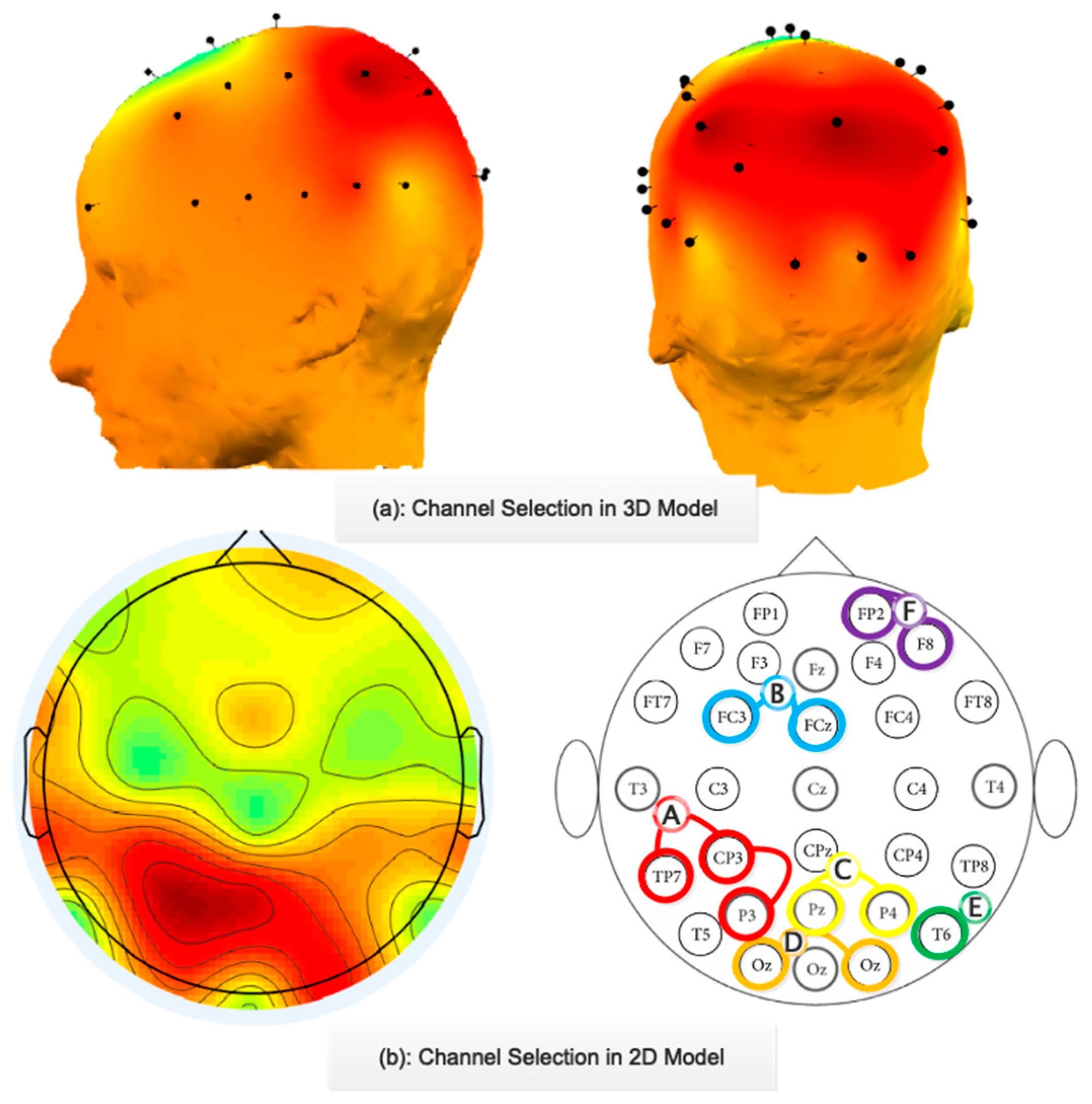
• Selecting active regions to reduce computational complexity.
• Compiling a complete dataset in accordance with stated norms.
• Developing a deep CNN–LSTM network capable of obtaining promising outcomes in all areas in the analyzed dataset.

The following is the remainder of the paper: Section 2 explains how to collect EEG data using a mathematical foundation in the CNN and LSTM disciplines. Section 3 deals with the method proposed. Section 4 presents the simulation outcomes and compares the present study with recent studies. Section 5 examines the advantages and disadvantages of the suggested methodology and suggestions for future work. Finally, the conclusion is dealt with in Section 6.

2. Materials and Methods

This section provides an overview of the University of Tabriz’s EEG data collection studies. A summary of deep CNN and LSTM networks was presented.

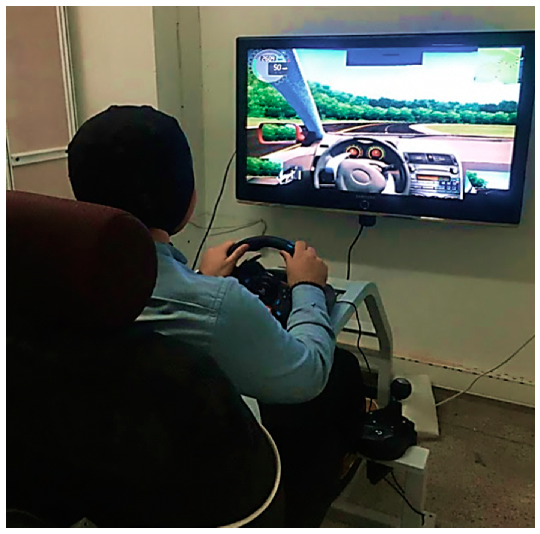
2.1. Acquisition of EEG Data

Eleven graduate students ranging in age from 22 to 30 years old participated in a driving simulation assessment. All participants were required to have a valid driver’s license and to never have driven in a driving simulator before. The experiment’s participants were all right-handed. A moral license number IR.TBZ-REC.1399.6 was issued to experiment with at the Biomedical Engineering Department’s Signal Processing Laboratory at the Faculty of Electrical and Computer Engineering, University of Tabriz. Before the experiment, all respondents were invited to freely confirm their participation by completing a permission form and recognizing the exam conditions (no history of psychiatry, epilepsy, or fatty food, pre-testing hair washing, adequate sleep throughout the night, and no pre-testing coffee). The experiment utilized a G-Tec 32-channel EEG recorder, an MSI laptop (Corei7 and 16 GB of RAM), a Logitech G29 Driving Simulator, a City Car Driving Simulator, and a Samsung 40-inch LCD. Figure 1 depicts the subject’s EEG signal recording during driving in the simulator. The EEG signal was recorded using the worldwide standard 10–20 electrode placement technique, with a sampling frequency of 1000 Hz and two A1 and A2 channels as reference electrodes. Before the experiment, all participants utilized the simulator to familiarize themselves with the device and the objective assessment. The driving path in the simulator was designed to simulate a uniform highway with no traffic to create mental fatigue in the driver. The final 3 min EEG data were classified as a normal stage, while the driving process lasted 20 min. The driving procedure continued for 60–100 min, or until the participant’s questionnaire, until findings (MFI scale) indicated that the subject had reached the driver’s fatigue stage. The subject’s final three minutes of EEG recordings were labeled as fatigue.

Two techniques were used to confirm fatigue: 1. decreasing performance, such as rising crash rates and highway deviations, and 2. the Chalder fatigue [30] and the Lee fatigue scales [31]. These questionnaires included the preceding questions: Is it necessary for you to rest? Are you exhausted? Do you suffer from blurred vision? Do you have a sense of deficiency? Each question was worth four points, ranging from −1 to 2. In addition, each score had the following interpretations: Score −1 indicated that something was better than usual, 0 implied that something was normal, 1 indicated that something was worse than usual, and 2 implied that something was considerably worse than expected. A high fatigue score implies a high degree of driving fatigue and has been employed to corroborate driver fatigue in several current investigations [32,33,34]. Previous studies did not refer to the sound of the car engine when recording the EEG signal. They did not consider this critical parameter to reduce the accuracy of their algorithm.

In contrast to previous studies, we also considered the sound of the car engine when recording the EEG signal. It was necessary to consider all parameters of the driving environment to navigate the present study to the practice field. For each topic, the driving task began at 9:00 a.m. Each day, just one EEG signal was captured to verify that the recording time was consistent. The raw EEG signal obtained from the two electrodes, FC3 and FCZ, related to two states of fatigue and normal, is illustrated in Figure 2. According to Figure 2, the visual distinction between fatigue and normal stages is difficult. It depended on the experience and expertise of the expert, which indicated the need to design automatic detection of driver fatigue systems based on EEG signals.

2.2. An Overview of the Deep Convolutional Neural Network (CNN)

The CNN is a deep learning method in which multiple layers are trained in a powerful way. There are three main layers of a CNN: the convolution layer, the pooling layer, and the fully connected layer. Each of these layers has different tasks. In each CNN, there are two stages of training: feed-forward and back-propagation. In the first stage, the input signal enters the network and this step involves multiplying the point between the input and the parameters of each neuron and performing convolution operations. The output of the network is then calculated. The output is used to set network parameters or training to calculate a network error. The output error of the network is compared to the correct answer and the final error value is obtained. Based on the calculated error rate, back-propagation would begin in the second stage. In the second step, each parameter’s gradient is determined in accordance with the chain rule, and all parameters change their values according to their error effect. After updating the parameters, the feed-forward step begins. The network training ends with the proper repetition of these steps [35,36,37].

The CNN is a hierarchical network in which the convolutional layers are joined one by one with pooling layers and then a number of fully connected layers are placed. This layer uses a variety of filters to convolution the input signal, resulting in a variety of feature maps. The pooling layer is commonly positioned after the convolution layer and is used to reduce the size of the network feature map and parameters. Pooling layers, such as convolution layers, are fixed relative to translation. The average-pooling and max-pooling functions are known as the most common implementation functions of this layer. In this study, the max pooling function was used due to achieve a faster convergence and better generalization in the proposed network architecture. The fully connected layer allowed us to present the result of the network in the form of a vector with a specified size [37,38].

The loss function determined the error ratio during the prediction stage. Following that, an optimization technique was used to minimize the error criteria. Optimization findings were employed to update hyper-parameters. The loss function is used in machine learning algorithms to evaluate and describe model efficiency [31,35]. Generally, CNNs employ the cross-entropy loss function, which is described as follows [35,39]:

$$C_{ij}={\displaystyle \sum _n^{}\left(P_{ij}^{*}\times \log P_{ij}^{}-\left(1-P_{ij}^{*}\right)\times \log \left(1-P_{ij}^{}\right)\right)}$$

(1)

The amount of cross-entropy loss between i and j is denoted by $C_{ij}$. The probability distribution of the output classes determined using the SoftMax activation function is represented by $P_{ij}^{*}$, and the number of classes is denoted by $n$.

2.3. Brief Description of Long Short-Term Memory (LSTM) Network

A particular type of recurrent neural network (RNN) capable of learning long-term dependencies is the LSTM network. The aim of designing LSTM networks is to solve the problem of long-term dependency. All standard RNNs are repetitive sequences of ANN modules. As a result, LSTM networks are no exception to this rule. However, unlike RNNs with a layer such as tanh, LSTM networks have four layers that interact according to a specific structure. These networks can add new information to their cell and delete additional information. This is performed by employing precise structures called gates. Gateways are a means of entering information that consists of a sigmoid layer of a neural network with a point multiplication operator. The output of the sigmoid layer is a number between zero and one that indicates how much input is to be sent to the output. A value of zero indicates that no information should be sent to the output, while a value of one indicates that all inputs should be passed to the output [39,40].

These networks also have three similar gates to control the number of cells. The initial stage in these networks is to determine which information should be removed from the cell. The decision is determined by the forget gate, a sigmoid layer. Depending on the X_t and h_t−1 values, this gate takes the value of zero or one in cell C_t−1 to output. A value of one means that the total value of the cell C_t−1 has to be passed to C_t, and a value of zero means that the data of the current C_t−1 cell have to be deleted, and no value has to be passed to C_t. They were conducted in the form of Equation (2).

$$f_t=\sigma (w_f·[h_{t-1},x]+b_f)$$

(2)

The next stage determines what additional data should be stored in each cell. This is a two-part decision, and it works such as this: Firstly, we had the entry gate, a sigmoid layer that determined how much to update. The next step was a tanh layer that formed a vector of values called ${\tilde{C}}_t$, and could be added to the cell. These two steps were combined to update the number of cells as follows:

$$i_t=\sigma (w_t·[h_{t-1},x]+b_i)$$

(3)

$${\tilde{C}}_t=\tanh (w_c·[h_{t-1},x]+b_c)$$

(4)

The old C_t−1 cell was also updated to the new C_t cell: the previous cell value was multiplied by f_t to forget the information, and then i_t × $\tilde{C}$_t was added to it. New cell values were now obtained based on decisions already taken. They are performed in the form of Equation (5).

$$C_t=f_t\times C_{t-1}+i_t\times {\tilde{C}}_t$$

(5)

Finally, in the last stage, it had to be decided which information should be taken to the output. The output’s value should have been calculated based on the cell’s value; however, it had to additionally pass through a certain filter. The sigmoid layer first determined which section of the cell would be output, and then passed the cell value to the tanh layer (the values were between −1 and +1). Its value was multiplied by the preceding sigmoid layer’s output, so that only the sections we desired were output (h_t). These steps are shown in Equations (6) and (7) [39,40].

$$O_t=\sigma (w_O·[h_{t-1},x]+b_O)$$

(6)

$$h_t=\tanh \left(C_t\right)\times O_t$$

(7)

3. Proposed Method

This part outlines the suggested system’s phases for automatically detecting driver fatigue based on the proposed deep CNN–LSTM network. Figure 3 demonstrates the general structure of the suggested system. This section was divided into two subsections: data preprocessing and design of the proposed deep CNN–LSTM network architecture. Details of each subsection were explained below.

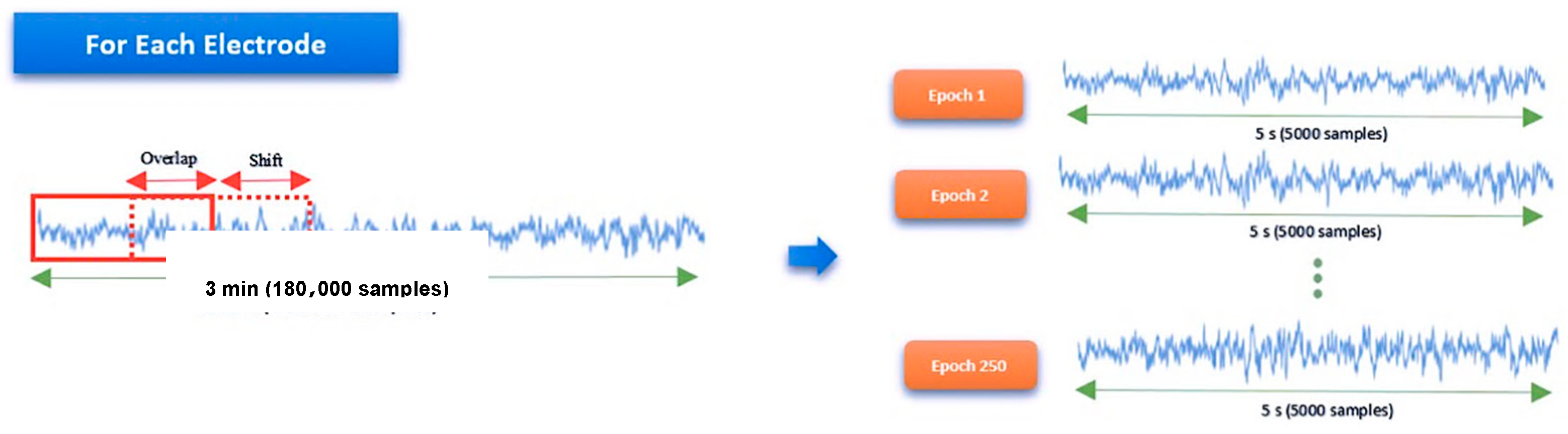
3.1. Data Preprocessing

A notch filter was employed initially, followed by a first-order Butterworth low-pass filter with a frequency of 0.5 to 45 Hz to eliminate the 50 Hz frequency of the power supply from data. Third, the features of each participant were standardized using a scale of 0 to 1 and the min–max method [41,42,43,44,45,46,47,48] to optimize detection quality with a time-saving strategy. It is essential to determine which EEG channels were active to develop a system that used the minimum possible number of EEG channels. To this end, an ICA algorithm was used in EEG Lab ver. 15 (MATLAB Toolbox) to identify active regions. Figure 4 shows the active areas of the ICA algorithm with selective electrodes in two dimensions, 2D and 3D.

As illustrated in Figure 4, six areas of the brain (A, B, C, D, E, and F) were employed for the automated identification of driver fatigue; consequently, the simulation used just those six regions (A, B, C, D, E, and F). According to Figure 4, the distribution of selected electrodes was not dispersed, as previously demonstrated in previous studies. A detailed interpretation of the selected regions can be found in [48], which shows that the EEG bursts were uniform when driving in the central and posterior regions. In addition, from the point of view of the EEG signal frequency analysis, it can be stated that theta and gamma rhythms increased with increasing fatigue, particularly in the central and forehead areas, and beta rhythms increased with decreasing consciousness in the posterior regions. Fifth, the suggested technique selected three minutes of the recorded signal for normal and fatigue phases for every channel. In such a scenario, we possessed two classes of data (180,000 dimensions) for every channel. Then, with the overlap method to avoid over-fitting, the data in each channel were divided into 5-second intervals. Accordingly, every electrode was separated into 250 samples based on the size of the shift, so we had $n\times 250\times 5000$, where $n$ is the number of electrodes. Since there were 11 subjects and two classes (normal and fatigue) in this study, the final dimension of the network input matrix would be equal $(2\times 11\times 250)\times (n\times 5000)$. Figure 5 shows overlap operation.

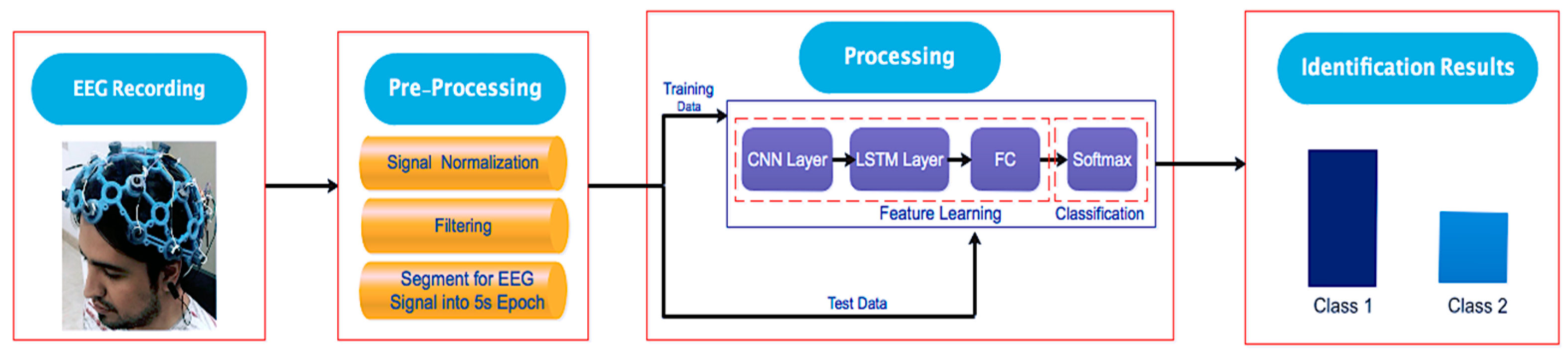
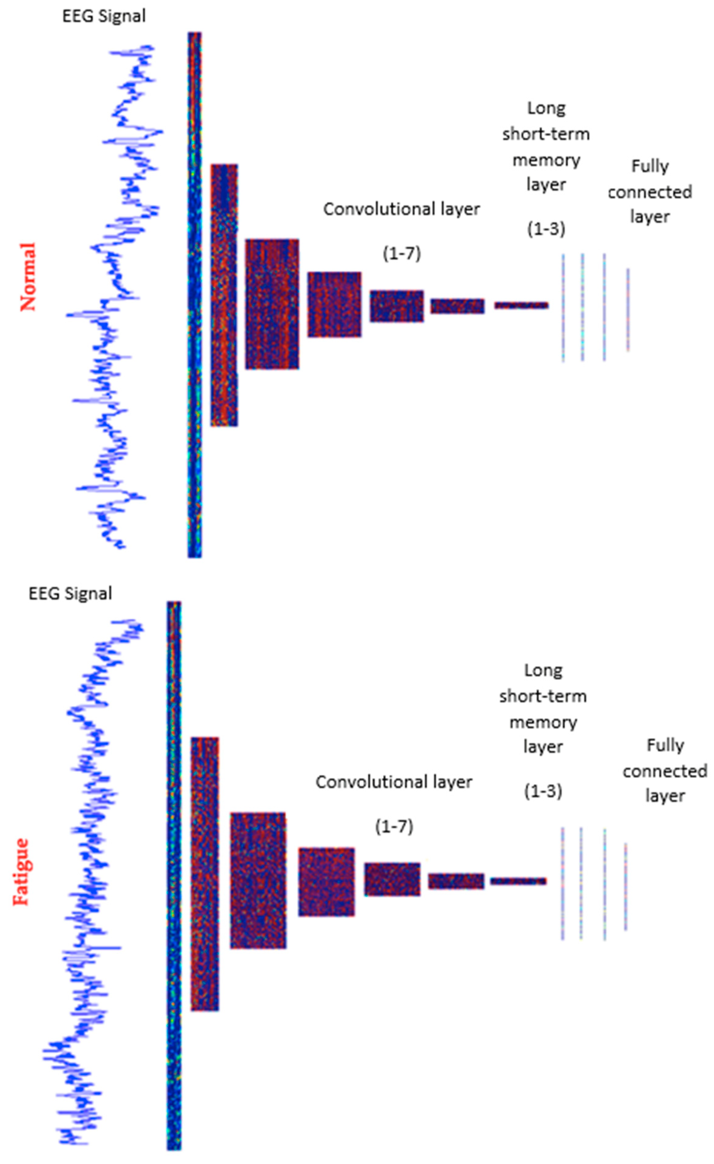
3.2. Proposed Deep CNN–LSTM Network Architecture

The suggested network architecture utilized a cross-library in the Python programming language to combine seven convolutional 1D layers and three LSTM layers. The fusion of the LSTM network with the CNN network increased stability and reduced oscillation. The details of the proposed deep network architecture for region E are offered in

Table 1. The details of the suggested network.

Padding	Number of Filters	Strides	Size of Filter and Pooling	Output Shape	Activation	Layer Type	L
					Function
Yes	16	8 × 1	128 × 1	(None, 625, 16)	Leaky-ReLU	Convolution1-D	0–1
No	-	2 × 1	2 × 1	(None, 312, 16)	-	Max Pooling1-D	1–2
Yes	32	1 × 1	3 × 1	(None, 312, 32)	Leaky-ReLU	Convolution1-D	2–3
No	-	2 × 1	2 × 1	(None, 156, 32)	-	Max Pooling1-D	3–4
Yes	64	1 × 1	3 × 1	(None, 156, 64)	Leaky-ReLU	Convolution1-D	4–5
No	-	2 × 1	2 × 1	(None, 78, 64)	-	Max Pooling1-D	5–6
Yes	64	1 × 1	3 × 1	(None, 78, 64)	Leaky-ReLU	Convolution1-D	6–7
No	-	2 × 1	2 × 1	(None, 39, 64)	-	Max Pooling1-D	7–8
Yes	64	1 × 1	3 × 1	(None, 39, 64)	Leaky-ReLU	Convolution1-D	8–9
No	-	2 × 1	2 × 1	(None, 19, 64)	-	Max Pooling1-D	9–10
Yes	64	1 × 1	3 × 1	(None, 19, 64)	Leaky-ReLU	Convolution1-D	10–11
No	-	2 × 1	2 × 1	(None, 9, 64)	-	Max Pooling1-D	11–12
Yes	64	1 × 1	3 × 1	(None, 9, 64)	Leaky-ReLU	Convolution1-D	12–13
No	-	2 × 1	2 × 1	(None, 4, 64)	-	Max Pooling1-D	13–14
-	-	-	-	(None, 128)	Leaky-ReLU	LSTM	14–15
-	-	-	-	(None, 128)	Leaky-ReLU	LSTM	15–16
-	-	-	-	(None, 128)	Leaky-ReLU	LSTM	16–17
-	-	-	-	(None, 100)	Leaky-ReLU	FC	17–18
-	-	-	-	(None, 2)	SoftMax	FC	18–19

and Figure 6. The dimensionality decrease in the hidden layers progressed from 5000 (the number of starting features) to 100, as shown in Table 1 and Figure 6 (selected feature vector). Ultimately, to compute scores, the chosen feature vector was connected to an FC layer using the SoftMax activation function. The stride length in the first layer of the proposed network was considered different for various regions. As can be seen, a large-sized filter was considered in the first layer of the proposed network, which helped to overcome high-frequency noises. Filters with small sizes were also used in the next layers of the proposed network, which would result in a better representation of input data. It should be mentioned that the values for hyper-parameters were adjusted, relying on a study of relevant investigations and tests performed on them. Finally, the Cross-entropy loss function and Adam optimizer [49] with a learning rate of 0.001 were selected for the training process. The total number of parameters for region E was 102,878. The total number of samples for each region was 5500; 2750 samples (50%) were randomly selected for network training, 550 samples (10%) were used for validation, and 2200 samples (40%) were used for testing. EEG data distribution for training, validation, and testing is depicted in Figure 7.

4. Results

The simulation results of the proposed method, a comparison with previous research, the advantages and disadvantages of the proposed method, and suggestions for future research were presented in this section.

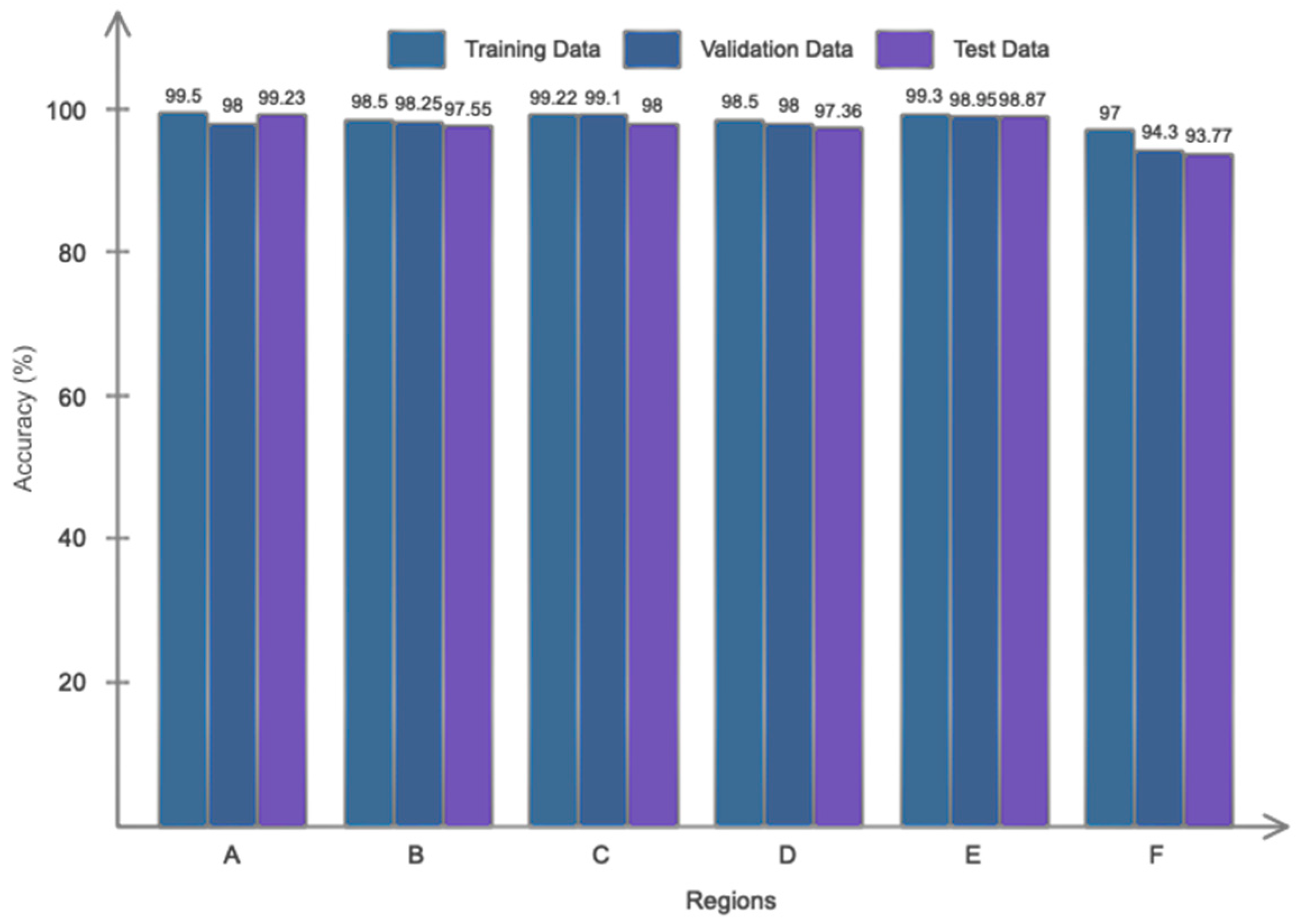
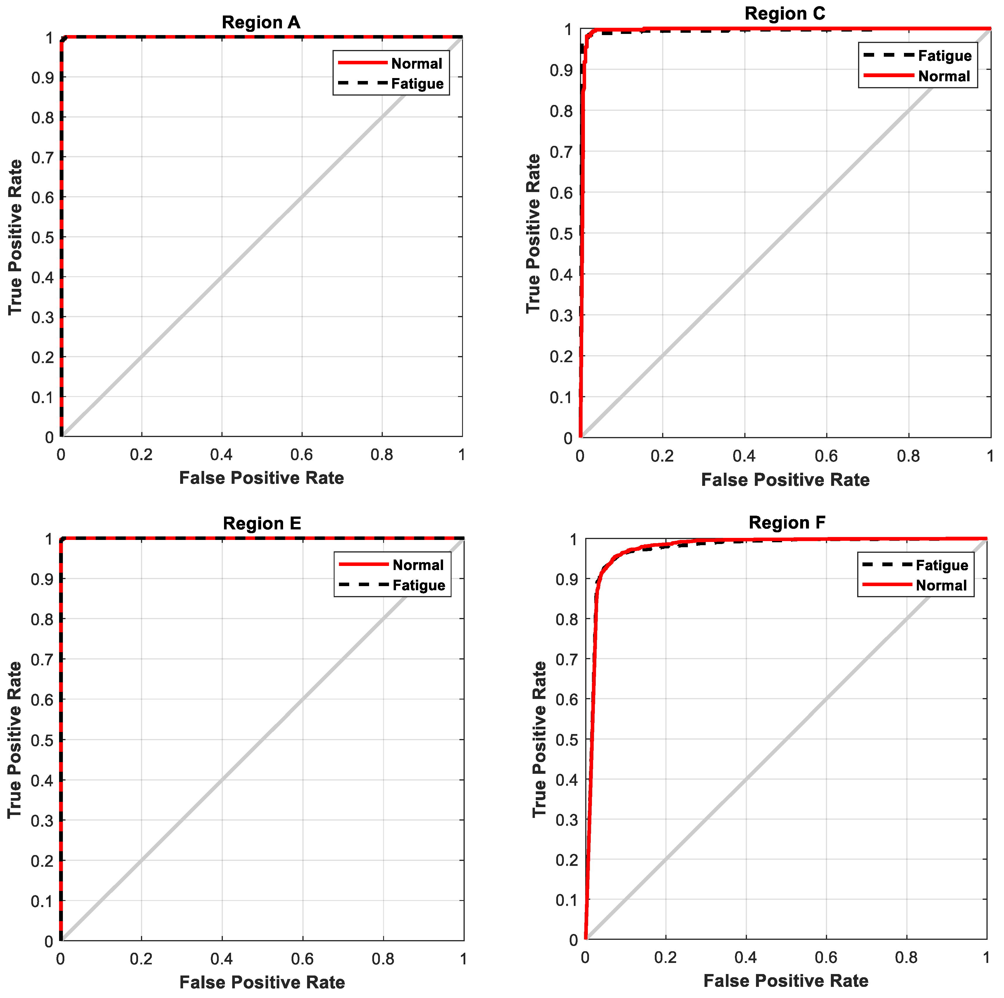
4.1. Obtained Results

The system specifications used included 8 GB of RAM and a 2.4 GHz CPU. Figure 8 shows the proposed network error for all regions for validation data. As illustrated in Figure 8, the network error for all areas decreased as the number of iterations increased and achieved a steady-state value around the 75th iteration. Figure 9 indicates the suggested method’s accuracy for all areas of validation data. In accordance with this figure, the suggested technique for two-stage categorization of driver fatigue had an accuracy of 99.23%, 97.55%, 98.00%, 97.36%, 98.78%, and 93.77% after approximately 75 iterations for areas A, B, C, and D. The confusion matrix for the two-stage categorization of all areas for testing data is shown in Figure 10 to allow for a more detailed analysis of the suggested technique. As can be seen, the accuracy achieved by the proposed method for region E was promising. In addition, as shown in Figure 10, as can be seen from the confusion matrix for the single-channel region (E), out of 1093 samples, only 17 samples were incorrectly detected, demonstrating the adequate performance of the suggested network architecture. It may be utilized to develop an autonomous driver fatigue detection system to achieve a high execution rate. In addition, Figure 11 depicts a bar chart depiction of accuracy in the training, validation, and testing processes for all areas. Figure 12 illustrates the receiver operating characteristic (ROC) curve analysis of the suggested approach for evaluating data from areas A, C, E, and F. According to Figure 12, the curved position was in the left hemisphere for all regions.

Moreover, Figure 13 demonstrates the t-sen diagram of the raw signal, Conv3, Conv7, LSTM1, LSTM3, and FC1 layers for the testing data of region E. The final layer indicated that all samples were properly segregated, revealing that the suggested technique performed well in two-stage classification.

Table 2. The kappa coefficient of the suggested method for all regions.

Region	A	B	C	D	E	F
Kappa	0.98	0.96	0.97	0.96	0.98	0.92

displays the kappa coefficient of the suggested approach for the two-stage categorization of driver fatigue for all locations.

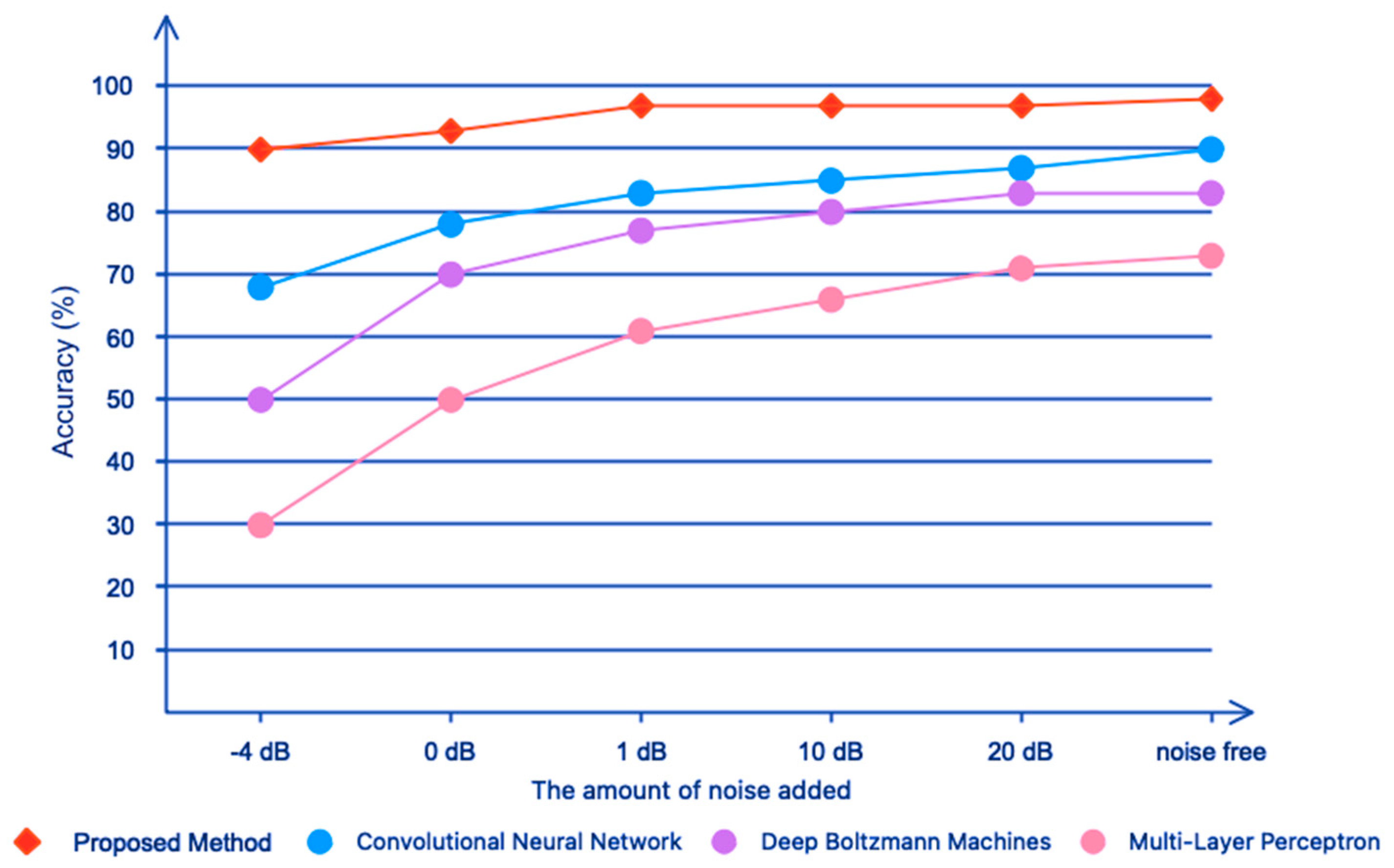
4.2. Comparison of the Proposed Method with Recent Research and Methods

The comparison of methods was conducted in two different sections: 1. comparison of the proposed method to recent research; 2. comparison of the proposed method with the different methods of extraction/selection and classification of features. Several automatic detections of driver fatigue methods were proposed using EEG signals in recent years. In

Table 3. Performance of the suggested method compared to different two-stage classification studies.

Research	Feature Method	Accuracy (%)
Correa et al. [16]	Multimodal Analysis	83
Xiong et al. [17]	Attitudinal Entropy and State Entropy	90
Chai et al. [18]	Entropy Rate Bound Minimization Analysis	88.2
Zhang et al. [19]	Entropy and Complexity Measure	96.5
Yin et al. [20]	Fuzzy Entropy	95
Ko et al. [21]	Fast Fourier Transform	90
Wang et al. [22]	Power Spectral Density	83
Mu et al. [23]	EEG Frequency Ratio	85
Nugraha et al. [24]	EMOTIV	96
Hu et al. [25]	Multiple Entropy	97.5
Min et al. [26]	Multiple Entropy	98.3
Cai et al. [27]	Horizontal Visibility Graph	98
Luo et al. [28]	Adaptive Scaling Factor and Multiple Entropy	95
Gao et al. [29]	Convolutional Neural Network	95
Proposed Method	Convolutional Neural Network–Long Short-Term Memory	99.23

, the accuracy of the proposed method is compared with different two-stage classification studies based on EEG signals. It is clear from Table 3 that the proposed method offered a greater degree of accuracy for the two-stage categorization of driver fatigue among all the comparative methods. The two-stage classification accuracy was 99.23%, while in [25,26], accuracies of 97.5% and 98.3% were reported for the same scenarios. The feature extraction was performed automatically based on deep learning from raw EEG data in the proposed method.

In contrast, traditional techniques based on manual features were used in comparative methods. However, it seemed that, despite the same scenarios, a one-to-one comparison of the proposed method with previous research was not fair because of existing uncertainties, such as varying measurement instruments and ambient circumstances. As a result, it was required to assess the suggested strategy in noise and no noise environmental conditions with other methods with the same data.

To demonstrate the efficient effect of the proposed method, we compared the performance of our method with CNN, DBM [50], and MLP [51], based on two different modes of operation (feature learning using raw data and manual feature learning) for region E (single-channel). Such networks have been commonly utilized to conduct experiments on automated driver fatigue detection in recent years. For this purpose, the CNN network architecture was carried out without considering the LSTM networks, as set out in Table 1. For the MLP and DBM networks, three hidden layers with a learning rate of 0.001 were considered. Maximum, skewness, variance, minimum, mean, crest factor, and kurtosis were also used as manual features [52,53]. The accuracy of the classification of the proposed method based on CNN–LSTM compared to the different methods is shown in

Table 4. Classification accuracy of the suggested method compared with other methods of comparison.

Methods	Feature Learning from Raw Data	Manual Features
Proposed Method	98.78%	80.35%
Convolutional Neural Network	90.26%	80.64%
Deep Boltzmann Machine	84.82%	77.78%
Multi-Layer Perceptron	73.45%	79.83%

. As shown in Table 4, the proposed CNN–LSTM, depending on feature learning from raw data, was able to show the best performance compared to other comparable networks, indicating the unique and desirable design of the network architecture.

According to the same table, as we can see, deep networks such as CNN–LSTM, CNN, and DBM showed better results depending on feature learning from raw signals compared to feature learning from manual features. As a result, we inferred that deep learning networks do not need a previous understanding of the issue/theme. However, according to Table 4, based on feature learning with manual features, the CNN–LSTM, CNN, and DBM networks showed a relatively similar performance. Figure 14 compares the suggested CNN–LSTM network to the comparable networks in terms of accuracy in applying feature learning from primary data in 100 iterations. According to this figure, the proposed network had a high convergence speed, low oscillation (due to the presence of the LSTM network), and high classification accuracy compared to the comparable networks. The time required for the training and testing of the proposed CNN–LSTM and similar networks is shown in

Table 5. Classification accuracy of the suggested method compared with other methods of comparison.

Methods	Proposed Method		Convolutional Neural Network		Deep Boltzmann Machine		Multilayer Perceptron
Region	Train	Test	Train	Test	Train	Test	Train	Test
A	1890 s	5 s	1030 s	3 s	911 s	4.5 s	100 s	2.5 s
B	1870 s	5 s	1011 s	3.5 s	801 s	4.5 s	82 s	2 s
C	1820 s	4 s	1100 s	4 s	800 s	4 s	80 s	1.5 s
D	1892 s	4.5 s	1008 s	3 s	810 s	4 s	77 s	1.5 s
E	1800 s	4 s	1002 s	3 s	680 s	3.5 s	67 s	1 s
F	1810 s	4.5 s	1004 s	3.5	672 s	3 s	79 s	2 s

for all active regions. Table 5 shows that the suggested network’s training time was greater than the alternatives. The test time for the proposed network was also acceptable compared to other networks. However, there was no need to worry because, with the advent of new graphics processing units (GPUs) and their use for processing, the learning time problem for deep learning networks was completely resolved. The minimum time required for training and testing is related to the MLP network. Still, as shown in Table 5 and Figure 14 above, the classification accuracy according to that network was not within acceptable limits.

Environmental circumstances do not remain constant when driving; thus, the suggested approach must be evaluated in ambient sounds such as vehicle engine noise and driver behavior while driving to determine assumptions that are more realistic. White Gaussian noise was introduced to the testing data with varying SNR levels to assess the performance of the various techniques (i.e., suggested approach, CNN, DBM, and MLP) in the existence of environmental noises (−4 to 20 dB). The test accuracy of the proposed method, CNN, DBM, and MLP networks based on feature learning for each SNR is shown in Figure 15. As can be seen, the proposed method, CNN, DBM, and MLP were robust to environmental noise, respectively, up to SNR ≤ 0 dB, SNR ≤ 1, SNR ≤ 10, and SNR ≤ 20, such that their accuracies were still approximately 90%, 80%, 80%, and 70%. As a result, it may be claimed that the suggested technique, outperforming CNN, DBM, and MLP, was also more resistant to environmental noise. The amazing architecture of the proposed network in the first layer of a large-sized filter was used to overcome high-frequency noises. Based on the available evidence, it can be stated that the proposed method could also be used for noisy data.

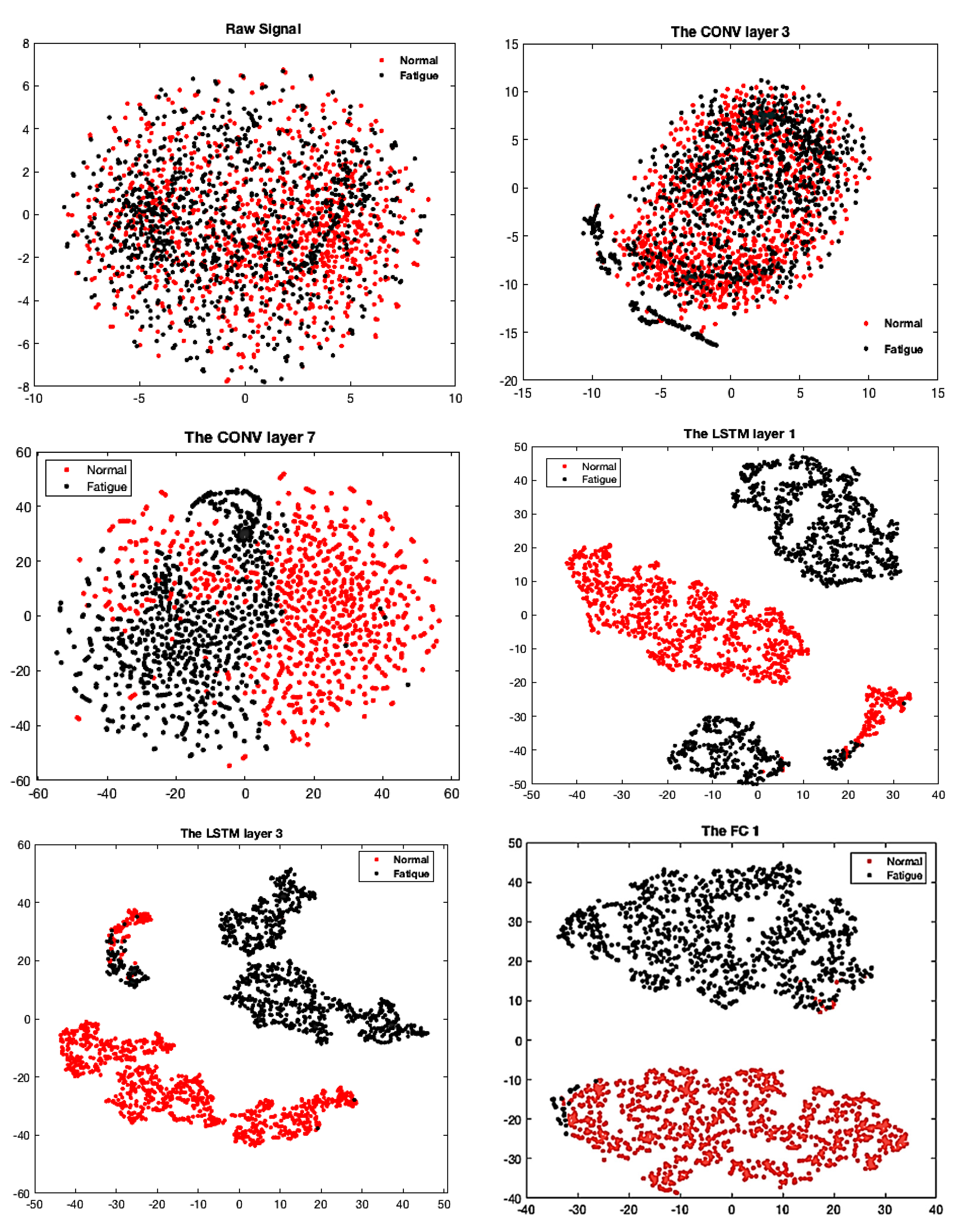
4.3. Intuitive Evaluation

The DNN is generally regarded as a black box. The internal operating mechanism of a DNN is difficult to understand, and none of the previous studies attempted to explore that, but to understand more, we tried to explore the internal activity of the proposed deep CNN–LSTM network by visualizing the activations in this network. First, we examined the reactions of the neurons in the first convolutional layer. Figure 16 shows the activations from the first convolutional layer for a sample of normal and fatigue states (region E). Sixteen convolutional kernels transformed the input signal 5000 × 1 into 625 × 16 maps, which were also called feature maps. It can be shown that the feature maps were different for two types of states, which showed that the first convolutional layer could learn the discriminant features of the raw EEG signals.

Second, to demonstrate what each layer could ‘sees’ in the proposed deep CNN–LSTM network for a sample of normal and fatigue states, the reactions of neurons of convolutional, LSTM, and FC layers were visualized. As shown in Figure 17, the size of the feature maps decreased with the exception of the first four layers, as the layer deepened. The powerful discriminating features learned from deep layers suggested the reasonableness to build a deep CNN–LSTM.

5. Discussion

As mentioned earlier, in recent years, many methods have been used to diagnose driver fatigue based on image-based methods, vehicle parameter-based methods, and physiological signal-based methods. However, image-based methods depend on brightness, and overshadow the privacy of the driver. Vehicle-based methods also depend on road marking and weather. For example, due to the coverage of road markings in snowy weather, these systems cannot perform well. Large companies such as Tesla have recently used vehicle parameters in the design of their vehicles, but reports of poor performance of embedded systems have also been reported. According to the above, the most reliable parameter for diagnosing driver fatigue can be considered the use of physiological signals such as EEG, because before causing fatigue in the driver, these signals change their nature. This change in the nature of the signals can be used to reliably detect driver fatigue. The present study was also designed on the basis of EEG signals. However, such as any other study, this study had advantages and disadvantages. The main advantages of the present study could be found in the design of the network architecture, which demonstrated good robustness to environmental noise. Additionally, as explained before (Section 2.1), previous research did not take into account the sound of the car engine when acquiring EEG data in order to not reduce the accuracy of its algorithm. In contrast to previous research, in order to present a more realistic study, we considered car engine noise in EEG signal acquisition and, as the simulation results showed, our proposed network was able to performance adequately because of its noise cancellation nature. Moreover, in view of the fact that the purpose of this study was to enter into a practical field, it is necessary to assess the different environmental conditions. The proposed algorithms in the field of driver fatigue detection must be able to remove noise in order to enter the field of application, because, as we know, driving is always subject to different environmental noises, such as driver behavior, music sound, car engine sound, etc.

The second advantage of the proposed method could be considered the provision of the active region, because to build real-time systems, it is necessary to reduce the computational complexity of the algorithm. For this purpose, as can be seen from Section 4, the accuracy of our classification based on the single-channel region (E) was over 97%. The method presented in this study was created to automatically detect driver fatigue on a small scale. In order to enter the field of application of the present research, it is necessary to present a study with a larger statistical population and more scenarios. Given the good performance of the proposed single-channel method, we predict that it can be used as a wearable hat for the driver while driving after being evaluated in a larger statistical community. In addition to reducing the computing volume, the design of a single-channel system would also result in driver comfort. Unfortunately, this goal was not achieved in this study due to the COVID-19 epidemic. For future research, we plan to consider more scenarios, including normal, semi-tired, tired, and alert, in a larger statistical community. We also plan to use the generative adversarial network (GAN) instead of the classic data increase (Section 3.1). Given the nature of these networks, we predict that the convergence rate of the network will increase to the desired value.

6. Conclusions

The objective of this study was to offer a unique approach for automatically detecting driver mental fatigue utilizing EEG signals in the presence of environmental noises, owing to a boost in road accidents caused by driver mental fatigue. A relatively comprehensive dataset was provided for two stages of mental fatigue (normal and fatigue). Moreover, a realistic approach was considered while developing the dataset based on stated criteria. A deep CNN–LSTM network was conceived and evolved to hierarchically extract characteristics from raw EEG data. The suggested network had seven CNNs, three LSTM layers, and two FC levels. The designed dataset was compared to manual features and intelligent networks, such as CNN, DBM, MLP, and CNN–LSTM. The suggested method’s findings indicated that it could learn features and provide acceptable detection outcomes. Compared to manual characteristics, the suggested strategy improved classification accuracy while relying less on expert knowledge. As previously noted, combining the CNN and LSTM networks improved the accuracy and stability of the suggested system in the case of feature learning.

We obtained a 98 percent accuracy for the single-channel region (E), which was rather promising compared to earlier techniques for autonomous driver fatigue identification. White Gaussian noise was utilized to test data with varying SNR levels to simulate environmental noises such as engine noise and driver behavior when driving to obtain results that were more realistic. The findings revealed that the suggested approach was more resistant to environmental noise than existing methods. Based on the findings, it can be concluded that the recommended approach for the automated identification of driver mental fatigue is ideal, and that it has the potential to minimize accidents and fatalities caused by driver mental fatigue if used.

References

1. World Health Organization. Global Status Report on Road Safety 2015; World Health Organization: Geneva, Switzerland, 2015. [Google Scholar]
2. Rau, P.S. In Drowsy driver detection and warning system for commercial vehicle drivers: Field operational test design, data analyses, and progress. In Proceedings of the 19th International Conference on Enhanced Safety of Vehicles, Washington, DC, USA, 6–9 June 2005; pp. 6–9. [Google Scholar]
3. Chacon-Murguia, M.I.; Prieto-Resendiz, C. Detecting Driver Drowsiness: A survey of system designs and technology. IEEE Consum. Electron. Mag. 2015, 4, 107–119. [Google Scholar] [CrossRef]
4. Sahayadhas, A.; Sundaraj, K.; Murugappan, M. Detecting driver drowsiness based on sensors: A review. Sensors 2012, 12, 16937–16953. [Google Scholar] [CrossRef] [PubMed] [Green Version]
5. Bengler, K.; Dietmayer, K.; Farber, B.; Maurer, M.; Stiller, C.; Winner, H. Three Decades of Driver Assistance Systems: Review and Future Perspectives. IEEE Intell. Transp. Syst. Mag. 2014, 6, 6–22. [Google Scholar] [CrossRef]
6. Rommerskirchen, C.P.; Helmbrecht, M.; Bengler, K.J. The Impact of an Anticipatory Eco-Driver Assistant System in Different Complex Driving Situations on the Driver Behavior. IEEE Intell. Transp. Syst. Mag. 2014, 6, 45–56. [Google Scholar] [CrossRef]
7. Sałapatek, D.; Dybała, J.; Czapski, P.; Skalski, P. Driver drowsiness detection systems. Zesz. Nauk. Inst. Pojazdów/Politech. Warsz. 2017, 3, 41–48. [Google Scholar]
8. Eichelberger, A.H.; McCartt, A.T. Volvo Drivers’ Experiences with Advanced Crash Avoidance and Related Technologies. Traffic Inj. Prev. 2013, 15, 187–195. [Google Scholar] [CrossRef]
9. Sommer, D.; Golz, M. In Evaluation of PERCLOS based current fatigue monitoring technologies. In Proceedings of the 2010 Annual International Conference of the IEEE Engineering in Medicine and Biology, Buenos Aires, Argentina, 30 August–4 September 2010; pp. 4456–4459. [Google Scholar]
10. Simons, R.; Martens, M.; Ramaekers, J.; Krul, A.; Klöpping-Ketelaars, I.; Skopp, G. Effects of dexamphetamine with and without alcohol on simulated driving. Psychopharmacology 2011, 222, 391–399. [Google Scholar] [CrossRef] [Green Version]
11. Das, D.; Zhou, S.; Lee, J.D. Differentiating Alcohol-Induced Driving Behavior Using Steering Wheel Signals. IEEE Trans. Intell. Transp. Syst. 2012, 13, 1355–1368. [Google Scholar] [CrossRef]
12. Verster, J.C.; Bervoets, A.C.; de Klerk, S.; Vreman, R.A.; Olivier, B.; Roth, T.; Brookhuis, K.A. Effects of alcohol hangover on simulated highway driving performance. Psychopharmacology 2014, 231, 2999–3008. [Google Scholar] [CrossRef]
13. Kar, S.; Bhagat, M.; Routray, A. EEG signal analysis for the assessment and quantification of driver’s fatigue. Transp. Res. Part F Traffic Psychol. Behav. 2010, 13, 297–306. [Google Scholar] [CrossRef]
14. Hua, X.; Ono, Y.; Peng, L.; Xu, Y. Unsupervised Learning Discriminative MIG Detectors in Nonhomogeneous Clutter. IEEE Trans. Commun. 2022, 57, 1–10. [Google Scholar] [CrossRef]
15. Horstmann, S.; Ramirez, D.; Schreier, P.J. Two-Channel Passive Detection of Cyclostationary Signals. IEEE Trans. Signal Process. 2020, 68, 2340–2355. [Google Scholar] [CrossRef]
16. Correa, A.G.; Orosco, L.; Laciar, E. Automatic detection of drowsiness in EEG records based on multimodal analysis. Med. Eng. Phys. 2014, 36, 244–249. [Google Scholar] [CrossRef] [PubMed]
17. Xiong, Y.; Gao, J.; Yang, Y.; Yu, X.; Huang, W. Classifying Driving Fatigue Based on Combined Entropy Measure Using EEG Signals. Int. J. Control Autom. 2016, 9, 329–338. [Google Scholar] [CrossRef]
18. Chai, R.; Naik, G.R.; Nguyen, T.N.; Ling, S.H.; Tran, Y.; Craig, A.; Nguyen, H.T. Driver Fatigue Classification with Independent Component by Entropy Rate Bound Minimization Analysis in an EEG-Based System. IEEE J. Biomed. Health Inform. 2017, 21, 715–724. [Google Scholar] [CrossRef]
19. Zhang, C.; Wang, H.; Fu, R. Automated Detection of Driver Fatigue Based on Entropy and Complexity Measures. IEEE Trans. Intell. Transp. Syst. 2013, 15, 168–177. [Google Scholar] [CrossRef]
20. Yin, J.; Hu, J.; Mu, Z. Developing and evaluating a mobile driver fatigue detection network based on electroencephalograph signals. Health Technol. Lett. 2016, 4, 34–38. [Google Scholar] [CrossRef]
21. Ko, L.-W.; Lai, W.-K.; Liang, W.-G.; Chuang, C.-H.; Lu, S.-W.; Lu, Y.-C.; Hsiung, T.-Y.; Wu, H.-H.; Lin, C.-T. In Single channel wireless EEG device for real-time fatigue level detection. In Proceedings of the 2015 International Joint Conference on Neural Networks (IJCNN), Killarney, Ireland, 12–17 July 2015; pp. 1–5. [Google Scholar]
22. Wang, Y.; Liu, X.; Zhang, Y.; Zhu, Z.; Liu, D.; Sun, J. In Driving fatigue detection based on EEG signal. In Proceedings of the 2015 Fifth International Conference on Instrumentation and Measurement, Computer, Communication and Control (IMCCC), Qinhuangdao, China, 18–20 September 2015; pp. 715–718. [Google Scholar]
23. Zhendong, M.; Jinghai, Y. Mobile Healthcare System for Driver Based on Drowsy Detection Using EEG Signal Analysis. Metall. Min. Ind. 2015, 4, 34–38. [Google Scholar]
24. Nugraha, B.T.; Sarno, R.; Asfani, D.A.; Igasaki, T.; Munawar, M.N. Classification of Driver Fatigue State Based on Eeg Using Emotiv Epoc+. J. Theor. Appl. Inf. Technol. 2016, 86, 54–60. [Google Scholar]
25. Hu, J. Automated Detection of Driver Fatigue Based on AdaBoost Classifier with EEG Signals. Front. Comput. Neurosci. 2017, 11, 72. [Google Scholar] [CrossRef] [Green Version]
26. Min, J.; Wang, P.; Hu, J. Driver fatigue detection through multiple entropy fusion analysis in an EEG-based system. PLoS ONE 2017, 12, e0188756. [Google Scholar] [CrossRef] [Green Version]
27. Cai, Q.; Gao, Z.-K.; Yang, Y.-X.; Dang, W.-D.; Grebogi, C. Multiplex Limited Penetrable Horizontal Visibility Graph from EEG Signals for Driver Fatigue Detection. Int. J. Neural Syst. 2019, 29, 1850057. [Google Scholar] [CrossRef] [Green Version]
28. Luo, H.; Qiu, T.; Liu, C.; Huang, P. Research on fatigue driving detection using forehead EEG based on adaptive multi-scale entropy. Biomed. Signal Process. Control 2019, 51, 50–58. [Google Scholar] [CrossRef]
29. Gao, Z.-K.; Li, Y.-L.; Yang, Y.-X.; Ma, C. A recurrence network-based convolutional neural network for fatigue driving detection from EEG. Chaos Interdiscip. J. Nonlinear Sci. 2019, 29, 113126. [Google Scholar] [CrossRef] [PubMed]
30. Jackson, C. The Chalder Fatigue Scale (CFQ 11). Occup. Med. 2014, 65, 86. [Google Scholar] [CrossRef] [PubMed] [Green Version]
31. Sheykhivand, S.; Rezaii, T.Y.; Meshgini, S.; Makoui, S.; Farzamnia, A. Developing a Deep Neural Network for Driver Fatigue Detection Using EEG Signals Based on Compressed Sensing. Sustainability 2022, 14, 2941. [Google Scholar] [CrossRef]
32. Craig, A.; Tran, Y.; Wijesuriya, N.; Nguyen, H. Regional brain wave activity changes associated with fatigue. Psychophysiology 2012, 49, 574–582. [Google Scholar] [CrossRef] [PubMed]
33. Desai, R.; Tailor, A.; Bhatt, T. Effects of yoga on brain waves and structural activation: A review. Complementary Ther. Clin. Pract. 2015, 21, 112–118. [Google Scholar] [CrossRef]
34. Ellis, R.S. Entropy, Large Deviations, and Statistical Mechanics; Taylor & Francis: Abingdon, UK, 2006; Volume 1431. [Google Scholar]
35. Goodfellow, I.; Bengio, Y.; Courville, A. Deep Learning; MIT Press: Cambridge, MA, USA, 2016. [Google Scholar]
36. Hung, S.-L.; Adeli, H. Parallel backpropagation learning algorithms on Cray Y-MP8/864 supercomputer. Neurocomputing 1993, 5, 287–302. [Google Scholar] [CrossRef]
37. Hinton, G.E.; Srivastava, N.; Krizhevsky, A.; Sutskever, I.; Salakhutdinov, R.R. Improving neural networks by preventing co-adaptation of feature detectors. arXiv 2012, arXiv:1207.0580. [Google Scholar]
38. Graves, A. Generating sequences with recurrent neural networks. arXiv 2013, arXiv:1308.0850. [Google Scholar]
39. Mousavi, Z.; Rezaii, T.Y.; Sheykhivand, S.; Farzamnia, A.; Razavi, S. Deep convolutional neural network for classification of sleep stages from single-channel EEG signals. J. Neurosci. Methods 2019, 324, 108312. [Google Scholar] [CrossRef] [PubMed]
40. Hochreiter, S.; Schmidhuber, J. Long short-term memory. Neural Comput. 1997, 9, 1735–1780. [Google Scholar] [CrossRef]
41. Mousavi, Z.; Ettefagh, M.M.; Sadeghi, M.H.; Razavi, S.N. Developing deep neural network for damage detection of beam-like structures using dynamic response based on FE model and real healthy state. Appl. Acoust. 2020, 168, 107402. [Google Scholar] [CrossRef]
42. Mousavi, Z.; Varahram, S.; Ettefagh, M.M.; Sadeghi, M.H.; Razavi, S.N. Deep neural networks–based damage detection using vibration signals of finite element model and real intact state: An evaluation via a lab-scale offshore jacket structure. Struct. Health Monit. 2021, 20, 379–405. [Google Scholar] [CrossRef]
43. Sheykhivand, S.; Mousavi, Z.; Rezaii, T.Y.; Farzamnia, A. Recognizing Emotions Evoked by Music Using CNN-LSTM Networks on EEG Signals. IEEE Access 2020, 8, 139332–139345. [Google Scholar] [CrossRef]
44. Sheykhivand, S.; Mousavi, Z.; Mojtahedi, S.; Rezaii, T.Y.; Farzamnia, A.; Meshgini, S.; Saad, I. Developing an efficient deep neural network for automatic detection of COVID-19 using chest X-ray images. Alex. Eng. J. 2021, 60, 2885–2903. [Google Scholar] [CrossRef]
45. Sheykhivand, S.; Rezaii, T.Y.; Mousavi, Z.; Delpak, A.; Farzamnia, A. Automatic Identification of Epileptic Seizures from EEG Signals Using Sparse Representation-Based Classification. IEEE Access 2020, 8, 138834–138845. [Google Scholar] [CrossRef]
46. Yousefi Rezaii, T.; Sheykhivand, S.; Mousavi, Z.; Meshini, S. Automatic stage scoring of single-channel sleep EEG using CEEMD of genetic algorithm and neural network. Comput. Intell. Electr. Eng. 2018, 9, 15–28. [Google Scholar]
47. Sheykhivand, S.; Rezaii, T.Y.; Saatlo, A.N.; Romooz, N. Comparison between different methods of feature extraction in BCI systems based on SSVEP. Int. J. Ind. Math. 2017, 9, 341–347. [Google Scholar]
48. Borghini, G.; Vecchiato, G.; Toppi, J.; Astolfi, L.; Maglione, A.; Isabella, R.; Caltagirone, C.; Kong, W.; Wei, D.; Zhou, Z.; et al. Assessment of mental fatigue during car driving by using high resolution EEG Activity and Neurophysiologic Indices. In Proceedings of the 2012 Annual International Conference of the IEEE Engineering in Medicine and Biology Society, San Diego, CA, USA, 28 August–1 September 2012; pp. 6442–6445. [Google Scholar]
49. Zhang, W.; Li, C.; Peng, G.; Chen, Y.; Zhang, Z. A deep convolutional neural network with new training methods for bearing fault diagnosis under noisy environment and different working load. Mech. Syst. Signal Process. 2018, 100, 439–453. [Google Scholar] [CrossRef]
50. Salakhutdinov, R.; Larochelle, H. In Efficient learning of deep Boltzmann machines. In Proceedings of the Thirteenth International Conference on Artificial Intelligence and Statistics, Sardinia, Italy, 13–15 May 2010; pp. 693–700. [Google Scholar]
51. Hsu, Y.-L.; Yang, Y.-T.; Wang, J.-S.; Hsu, C.-Y. Automatic sleep stage recurrent neural classifier using energy features of EEG signals. Neurocomputing 2013, 104, 105–114. [Google Scholar] [CrossRef]
52. Sabahi, K.; Sheykhivand, S.; Mousavi, Z.; Rajabioun, M. Recognition Covid-19 cases using deep type-2 fuzzy neural networks based on chest X-ray image. Comput. Intell. Electr. Eng. 2022, 87, 25–36. [Google Scholar]
53. Fedala, S.; Rémond, D.; Zegadi, R.; Felkaoui, A. Contribution of angular measurements to intelligent gear faults diagnosis. J. Intell. Manuf. 2015, 29, 1115–1131. [Google Scholar] [CrossRef]
Figure 1. A participant while driving in a driving simulator.
Electronics 11 02169 g001
Figure 2. A sample EEG signal collected from FC3 and FCZ electrodes in one experiment for subject 1.
Electronics 11 02169 g002
Figure 3. The block diagram for the suggested method.
Electronics 11 02169 g003
Figure 4. Select active channels in 2D and 3D models (region A = TP7, CP3 and P3; region B = FC3 and FCz; region C = Pz and P4; region D = O1 and O2; region E = T6; region F = FP2 and F8).
Electronics 11 02169 g004
Figure 5. The overlap operation for each electrode.
Electronics 11 02169 g005
Figure 6. The proposed network architecture.
Electronics 11 02169 g006
Figure 7. EEG data allocation for training, validation, and testing.
Electronics 11 02169 g007
Figure 8. The proposed network error for all regions for validation data.
Electronics 11 02169 g008
Figure 9. The proposed network accuracy for all regions for validation data.
Electronics 11 02169 g009
Figure 10. The confusion matrix for two-stage classification for regions A, B, C, D, E, and F.
Electronics 11 02169 g010aElectronics 11 02169 g010b
Figure 11. The bar chart diagram of proposed method for all regions.
Electronics 11 02169 g011
Figure 12. The receiver operating characteristic (ROC) analysis for regions A, C, E, and F.
Electronics 11 02169 g012
Figure 13. The t-sen diagram of the suggested method for single-channel region (E).
Electronics 11 02169 g013
Figure 14. The accuracy of the suggested method compared to the other networks.
Electronics 11 02169 g014
Figure 15. The test accuracy of the different methods based on feature learning for each SNR.
Electronics 11 02169 g015
Figure 16. Visualization of activations from the first convolutional layer for a sample of normal and fatigue states (region E).
Electronics 11 02169 g016
Figure 17. Visualization of convolutional, long short-term memory, and fully connected layers in the proposed deep network for a sample of normal and fatigue states.
Electronics 11 02169 g017