Abstract
Estimating the coupling properties between a radiating structure and other conductive elements, the field behavior of the radiating source is essential to know. One well-known classification of the field behavior are the field-regions around antennas, namely, the far-field, the radiating near-field, and the reactive near-field. The different kinds of near-fields are distinguished by the reactive and radiating parts of the electromagnetic field, whereas in the far-field region the field behaves as a plane wave in the direction of propagation. One way to describe these field characteristics is to use the complex Poynting vector, which defines the electromagnetic power flow. This work presents a Poynting-vector-based approach to classify and visualize the field behavior around simple radiators using numerical simulations. First, the approach is applied to simple antenna structures such as dipoles and loop antennas. Later, the introduced field regions are utilized to predict the coupling behavior of practical applications, the coupling between single elements of a linear antenna array, and the coupling behavior of an electrically large loop antenna. It could be shown that the introduced approach, defining a surface description of the boundary between the near-field regions, enables the possibility of predicting the coupling behavior between radiating structures. The introduced error estimator for the far-field also delivers knowledge about the far-field quality in different angular directions and distances. All simulations have been executed applying a one-dimensional partial element equivalent circuit method.
1. Introduction
For electromagnetic systems with alternating or pulsing currents, radiation effects arise. Consequently, every conducting structure with this kind of current can act as an antenna. To understand the radiation behavior and impact on neighboring elements, knowledge about the field properties around these radiating structures is crucial. A rough classification of the field behavior is made by introducing so-called field regions [1]. In doing so, the surrounding volume of the antenna is distinguished into three regions, described by a distance to the antenna itself. As shown in Figure 1, the immediate surrounding, enclosed by a sphere with the radius , is called the reactive near-field (NF). According to [1] (p. 23), the reactive energy predominates here. The next region, limited by a sphere with the radius , is called the radiative NF. In this region, the reactive field has mainly vanished, and the radiation behavior of the antenna is formed. Therefore, it is also called the transition zone. Outside , the far-field (FF) is located, where the angular field distribution is independent of the radius [1] (p. 15).
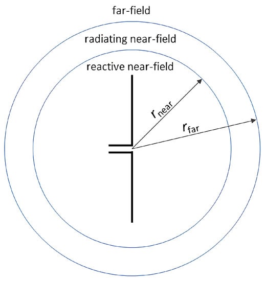
Figure 1.
Schematic view of an antenna and the surrounding field regions, described by the radii and .
For coupling mechanisms, the distinction of the field regions between reactive and radiative field components is essential. According to Figure 2, for electromagnetic interference (EMI), three kinds of electromagnetic coupling to neighboring elements are defined: radiated, conducting, and reactive interference. The last include inductive and capacitive effects [2]. Conductive interference is an effect based on galvanically coupled elements. As this work focuses on coupling through the air interface, these effects are not discussed in detail.
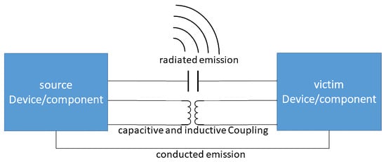
Figure 2.
Sketch of the different kinds of electromagnetic interference.
Radiated interference mainly occurs in the FF of a radiating structure, where the radiating field is predominant. Therefore, the affected surrounding can be estimated using the directivity of the radiating structure. From the EMI point of view, it is essential to know where radiated interference mainly occurs, and therefore deep knowledge about the FF region and its boundary is helpful. Hereby, the reaction on the source itself is usually minor for radiating emissions.
When another element is within the reactive NF region of a radiating structure, mainly reactive coupling can be observed. Depending on the geometry of the source and victim, this can be either capacitive or inductive coupling. From the emitting element’s point of view, it is crucial to know where the reactive power flow predominates and where reactive coupling happens. This region can be described with the knowledge of the boundary of a radiator.
For example, in [3,4], the radiative and reactive interferences are analyzed by examining the power flow between the radiator and victim to implement proper shielding structures. The exact knowledge of the directivity and highly reactive regions could help focus on potentially harmed victims.
Besides EMI considerations, knowing the NF boundary can be important when computing antenna systems. In [5], different computational methods for analyzing a linear antenna array have been examined. Among these methods, one neglects the mutual coupling effects mainly affected by reactive coupling. Therefore, deep knowledge of the reactive NF region can help choose the best computational method regarding accuracy and computation time.
First definitions of the radii and were introduced using the phase difference of two spatially separated radiation sources at a reference point , far away from the sources [6] (pp. 40–44). The phase difference between these two sources is based on the phase-term of the Green’s function for radiation problems and the different positions of the radiating sources , with k being the wavenumber. Using this approach, analytical expressions for and depending on the wavelength and the maximum dimension of the antenna l could be found [6] (pp. 40–44).
Besides this analytical approach, numerical methods based on error estimators, describing the FF quality depending on the distance to the radiation source, have been introduced in the last few years. These error estimators compare the actual field behavior with the ideal field behavior in the FF, which is based on Sommerfeld’s radiation condition.
In [7], the field regions of short dipoles are analyzed using an error estimator based on the wave impedance and an error estimator based on the electric field. In this case, for large distances to the antenna, the wave impedance has to converge to the wave impedance of free space . As in the FF, the radial component of the electric field has to vanish, and the quotient could be used to estimate the FF quality in a second analysis. Additionally, in [8], the wave impedance was used to estimate the FF behavior of dipole antennas. Additionally, the temporal phase between and is analyzed, which has to be zero in the FF. In [9], the wave impedance and a Poynting-vector-based approach were used to estimate the FF behavior of dipole antennas. In this work, an error-estimator based on the decreasing behavior of the tangential component of the Poynting vector was introduced. The work in [10] analyzed the FF quality and the boundaries and for dipole antennas, a dipole-antenna-based array, and loop antennas. In that work, the FF’s error estimator is based on the electric field components; in contrast, the error-estimator for is based on the radiating portion of the total power flow, based on the Poynting vector. This work also showed that the analytical expressions for the start of the FF in [6] (pp. 40–44) are an appropriate approximation.
In the present work, first, the net power flow and the oscillating power flow around simple antennas is visualized using the real part and the imaginary part of the time-harmonic Poynting vector. Later, error estimators based on the Poynting vector are introduced to analyze the field regions and the boundary between them. For the FF, a visualization of the FF quality is given to obtain knowledge of which angular direction an error is made at small distances to the antenna. For the boundary between the radiating NF and the reactive NF, a new approach is introduced. The gained knowledge is later applied to actual examples to predict the coupling behavior between radiating structures.
The work is structured as followed: This section gives an introduction of the topic. Section 2 discusses the theory of the Poynting vector, field regions, and the most fundamental radiator, the Hertzian dipole (HD). Section 3 investigates the field regions of dipole antennas and the impact of the NF on dipole-based antenna arrays. Section 4 shows the field behavior of simple loop antennas and the radiating and reactive coupling behavior of an electrically large loop antenna. Finally, Section 5 gives a conclusion and outlook on this topic. All simulations have been executed using a one-dimensional partial element equivalent circuit (PEEC) method [11].
2. Fundamentals and Theory
2.1. Poynting Vector
In general, the Poynting vector describes the directional electromagnetic power flow, where is the electric field intensity and the magnetic field intensity. When assuming the linear case, sinusoidal fields and using complex quantities and , the Poynting vector can be written as
In 1, it can be observed that the total power flow consists of a time-averaged power flow and an oscillating part with double the frequency. The time-averaged power flow motivates the introduction of the complex Poynting vector as
where the real part denotes the average power flow, and the imaginary part relates to the reactive energy and an oscillating power flow [12,13] (p. 265, p. 39).
2.2. Field Regions
According to Figure 1, the surrounding air region around an antenna is subdivided into three regions: the reactive NF, the radiating NF, and the FF. Each of these regions is defined using specific properties of the electromagnetic field. A radius from the antenna origin can be determined using the specified properties, describing each region’s boundary. Naturally, no abrupt change in the field behavior occurs at this radii, but, rather, a smooth transition can be observed. The most outer region, the FF, is defined as ”that region of the field of an antenna where the angular field distribution is essentially independent of the distance from a specified point in the antenna’s region” [1] (p. 15). In other words, in the FF region, the radiating wave acts as a plane wave in the direction of propagation. As shown, this region ranges from the radius to infinity. The next inner region, the radiating NF, is defined as ”that portion of the near-field region of an antenna between the far-field and the reactive portion of the near-field region, wherein the angular field distribution is dependent upon the distance from the antenna” [1] (p. 23). Hence, mainly radiating field components exist here, but in contrast to the FF, the wave is not solely propagating in the radial direction from the antenna origin. In this region, the radiation behavior of the FF is formed. The radiating NF region ranges from the radii to .
The most inner region, called the reactive NF, is defined as ”that portion of the near-field region immediately surrounding the antenna wherein the reactive field predomi- nates” [1] (p. 23). As denoted in the standard, here, the reactive energy dominates. This region is the direct surrounding of the antenna delimited by a sphere with the radius .
2.2.1. Boundary between the Radiating Near-Field and the Far-Field
According to [1] (p. 15), for electrically large antennas with an overall dimension , the boundary for the FF is defined as
For antennas with an overall dimension smaller than , the definition in 3 showed to be insufficient [6] (p. 42). Hence, other definitions which fulfill all FF requirements can be found. These are summarized and discussed in [6] (pp. 40–44) and given with
As in the FF region, the radiating part of the field has to be dominant, and the reactive part has to vanish, hence . Additionally, since the wave should propagate as a plane wave perpendicular to the sphere’s surface, the tangential component of the Poynting vector on the sphere’s surface has to vanish. Therefore, in the FF, only the real part of the radial component of the Poynting vector should be present, which leads to the estimation for the FF error :
Since no antenna system is omnidirectional, solid angles can be observed, where vanishes—consequently, it is necessary to extend 5. This is achieved by using the directivity [13] (pp. 44–58), which describes the normed radiation intensity of the antenna:
This error estimator will later be used to analyze the FF property qualitatively, and will denote regions where radiation effects can still be observable but will vanish with a higher distance.
2.2.2. Boundary between the Reactive and Radiating Near-Field
For the boundary , different definitions regarding the overall antenna dimension l can be found. According to [13] (p. 34), for electrically large antennas (), the boundary is defined as
Again, for electrically too small antennas, it could be shown that 7 underestimates the radius of the radiating NF region [6] (p. 42). A summary of the NF boundary is also discussed in this reference and can be given also for small antennas with
In contrast to the reactive NF region, the radiating field parts dominate in the radiating NF region. Assuming a closed surface of a sphere with the radius , when the reactive power flow through the enclosing surface equals the radiating power flow, the exchange of oscillating and radiating power through this surface is equal. Hence, according to the IEEE standard [1] (p. 23), this can be seen as the boundary between the two NF regions. To describe this relation, the factor is defined as
The NF boundary can then be described as the radius where
is fulfilled. It will later be shown when using 10, that for the field of an HD, the NF boundary mentioned in 8 will exactly be met for the whole sphere’s surface. In contrast, for more complex antennas, no exact sphere can be found where 10 is fulfilled for the entire surface. Hence, it is necessary to introduce the NF boundary in terms of the surface of a more general volume by introducing an angular dependent radius . Using the normal component of the power flow through the enclosing surface and introducing the error estimator ,
the more general NF boundary can be described by the radius , applying the constraint .
2.3. Hertzian Dipole
First, an HD is investigated to analyze the introduced error estimators and obtain basic knowledge about the power flow. An HD is a theoretical antenna concept of a z-orientated line-source with a constant oscillating current along a short length . In [13] (p. 34), the computation of the electric and magnetic field intensities is shown and given in spherical coordinates for the time-harmonic case:
where is the wave impedance of vacuum and k the wave number. Using 2 and 12, the complex Poynting vector of the HD can be computed:
When examining the power flow around the HD, shown in Figure 3 and stated in 13, it can be seen that the real part has pure radial components. Therefore, in this antenna concept, no radiating NF or so-called transition phase can be observed. The imaginary part of also has radial components, dominant for small distances r. Consequently, an oscillating exchange of energy between the antenna and the surrounding air is observable. Additionally, there is an oscillating power flow in -direction around the antenna, as can be seen in Figure 3b. The magnitude of the reactive power flow shows the shape of two kidneys.
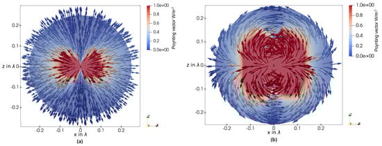
Figure 3.
(a) Real part of the Poynting vector around an HD in the E-plane, respectively, in the x/z plane. (b) Imaginary part of the Poynting vector around an HD in the E-plane.
In Figure 4, the error estimator for the NF, introduced in 9, applied on the HD is shown. It can be seen that the condition for the NF boundary stated in 10 is exactly met at the distance and shapes an exact sphere. With the modified error-estimator in 11, the same result would be present. This can also be derived by setting the real part of the radial component of the Poynting vector equal to the imaginary part of the radial component in 13.
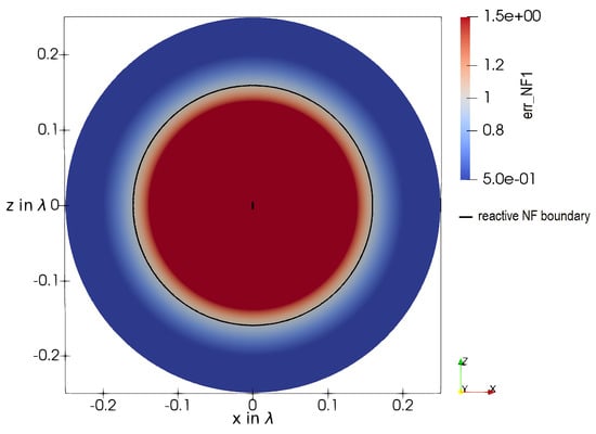
Figure 4.
The error-estimator 9, showing the reactive NF region around the HD in the E-plane.
Figure 5a shows the error estimator 5, describing the FF error around an HD. It can be seen that 5 is not applicable for solid angles, where the directivity , respectively, the real parts of , are zero. Consequently, 6 has been introduced, weighting 5 with the directivity to obtain a qualitative measure of the FF behavior. Examining Figure 5b, where the error-estimator 6 is applied on an HD, shows that the most significant error is made in regions between nulls and maximums of the directivity pattern. It can also be seen that the proposed FF boundary fits quite well for this kind of antenna, as the reactive power flow decayed and no transversal field components of the radiating part are present on the sphere’s surface.
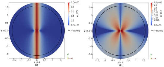
Figure 5.
(a) The error-estimator 5, describing the radial and real portion of the power flow applied on an HD in the E-plane. (b) The error-estimator 6 applied on an HD in the E-plane, describing the error-estimator weighted with the directivity . The FF boundary for very small antennas is displayed as a black circle.
3. Dipole Antennas and Dipole-Based Array
In this section, simple z-orientated dipole antennas are investigated. First, the power flow around the antenna is analyzed in detail. Second, the introduced error-estimators are applied to investigate the field behavior in the defined field regions. Subsequently, with the exact knowledge of the field regions, the coupling behavior of a linear dipole array is analyzed.
3.1. Dipole Antennas
This section analyzes the power flow and the proposed error estimators for the field regions for z-orientated dipole antennas with the overall lengths , , and .
In Figure 6, the real part (a) and the imaginary part (b) of the Poynting vector around a dipole is shown. Compared to the power flow of the HD in Figure 3, it can be seen that the real part has radial components and tangential components. The time-averaged power flow is almost normal to the antenna orientation near the antenna. However, this changes to the radial direction at a very short distance to the antenna. Hence, practically no transition zone is observable. For the imaginary part of the Poynting vector, thus, the oscillating part of the power flow, no qualitative difference is noticeable compared to the HD, and the same kidney shape of the magnitude is shown.
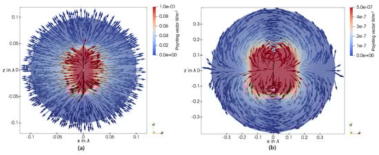
Figure 6.
(a) The real part of the Poynting vector in the E-plane of a dipole antenna with an overall length of . (b) The imaginary part of the Poynting vector in the E-plane of a dipole antenna with an overall length of .
Figure 7 shows the directivity (a) and the FF error-estimator 6 for a dipole antenna. For very small dipoles, such as the dipole, the directivity pattern and the maximum directivity are the same as for the HD [13] (p. 167). Additionally, the FF error behaves the same as for the HD. Hence, the FF boundary of fits well. The major errors are again made between the null and the lobe due to oscillating power flow.
In Figure 8, the real part (a) and imaginary part (b) of the Poynting vector of a dipole is shown. Compared to the dipole antenna, it can be seen that the transition zone is slightly more developed. Apart from that, the radiative power flow is qualitatively the same. Hence, a similar directivity pattern can be assumed. The imaginary part changes dramatically for larger dipole antennas. Now it seems as if two highly reactive regions are observable, with the upper and lower end of the antenna as the mid-points. This can be explained as the reactive energy of dipoles below behaving capacitively, and according to the transmission line theory on both ends, a voltage maximum occurs.
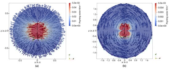
Figure 8.
(a) The real part of the Poynting vector in the E-plane of a dipole antenna with an overall length of . (b) The imaginary part of the Poynting vector in the E-plane of a dipole antenna with an overall length of .
Figure 9 indicates the directivity (a) and the FF error-estimator (b) for a dipole. Compared to the dipole and the HD, the maximum directivity grows to with a slightly narrower lobe. The error estimator for the FF shows a similar pattern to the one for small antennas. The magnitude is slightly lower at the FF boundary proposed in the literature. Again, the most significant error is made between nulls and lobes in the directivity pattern. The transition zone is more developed due to tangential field components of the real part of the Poynting vector.
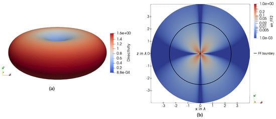
Figure 10 denotes the real part (a) and the imaginary part (b) of the Poynting vector around a dipole. From the real part, it can clearly be seen that the radiative power is flowing in different angular directions; hence, this antenna has not only one lobe. This again can be explained from transmission line theory, as the standing wave on the dipole has more than one maximum. A time-average power flow is observable between the lobes in the -direction, predominately towards the main lobe in the -direction. Consequently, here, the transition zone is more pronounced.
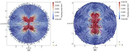
Figure 10.
(a) The real part of the Poynting vector in the E-plane of a dipole antenna with an overall length of . (b) The imaginary part of the Poynting vector in the E-plane of a dipole antenna with an overall length of .
The reactive power flow is more complex than for small antennas. The main oscillating power flow can be observed between lobes and nulls of the directivity pattern. Additionally, it can be clearly seen that the shape of the region with the dominant reactive power flow is not at all similar to a sphere. Hence, a simple radius definition of the reactive NF zone will be insufficient.
In Figure 11, the directivity (a) and the FF error (b) are shown for a dipole. It can be seen that, again, between lobes and nulls, the highest error arises. For larger antenna structures, such as that shown here, this is due to radiating field parts flowing in the tangential direction to the sphere’s surface, as shown in Figure 10a. The area where this happens is called the transition zone. Here, the FF error is relatively low at the literature’s proposed FF boundary. Hence, this can be seen as slightly overestimated.
In Figure 12, the proposed reactive NF region is shown for a (a) , (b) , and (c) dipole antenna. The regions have been derived with the error estimator 11 postulating . Hence, the oscillating power flow normal to the enclosing surface equals the time-averaged power flow.
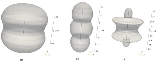
Figure 12.
The reactive NF region, described by the angular-dependent radius , when applying the error estimator 11 with of a (a) (b) , and (c) dipole. The corresponding dipole can be seen inside the region.
When investigating Figure 12a in detail, it can be seen that, compared to the HD, the former sphere stretched in the z-direction. As for the HD, the electric field is dominant. The maximum reactive power flow is close to voltage maximums along with the antenna structure. According to transmission line theory, this happens at the upper and lower end of a dipole antenna, which can be seen in the proposed region. The region seems similar to two overlapping spheres with a midpoint at the upper and lower end of the antenna.
In Figure 12b, the dipole length is . Here, another overlapping sphere can be seen at the feed-gap. As the structure has been excited with an impressed voltage, the feed gap also forms a capacitive structure; consequently, reactive power flow can be observed around it. Other than what is proposed in the literature [6] (p. 43), the proposed reactive NF region does not form a perfect sphere. In comparison, with the proposed region, the standard is met better regarding the reactive energy [1] (p. 23).
Figure 12c shows the reactive NF region of a dipole. Again, around the feeding structure and the end positions of the antenna, spherical structures can be observed. At an angle of about , a dent of the reactive NF region can be seen. This can be explained due to the low radiating power flow between the two lobes of the directivity pattern; hence, the reactive parts dominate for a longer distance.
3.2. Linear Antenna Array
This section analyzes a linear antenna array regarding the coupling behavior between the single elements. As shown in Figure 13, the array consists of five z-orientated dipoles equally spaced in the x-direction. All dipoles are excited with and no phase shift between the elements. To analyze the coupling behavior, the setting is analyzed in two ways. First, every element is computed separately using PEEC. The evaluated current on each dipole can later be used as a source to calculate a single element’s electromagnetic field. Using the pattern multiplication technique [13] (p. 286), the field of the array can later be evaluated by superposing the field parts of the single elements. As the dipoles are computed separately, no mutual coupling effects between the dipole elements are considered. Second, the array is solved at once, also using PEEC. Within this, the coupling behavior between the elements is considered. To obtain a quantitative measure of the coupling behavior, the currents of the single elements are compared. Additionally, the difference in the single elements’ impedance using the first proposed simulation method and the second one is made and visualized.
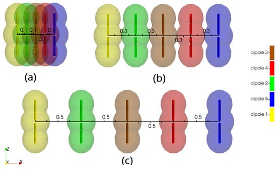
Figure 13.
The three investigated linear antenna arrays, each consisting of five -dipoles. The distance between these array elements is (a) , (b) , and (c) . The reactive NF region, proposed in Figure 12b, is shown around each dipole.
Here, we want to focus on the coupling behavior regarding the reactive NF. Three settings are analyzed in detail, as shown in Figure 13. Figure 13a shows the array with the spacing between the elements of . As can be seen, the reactive NF region overlaps, and a neighboring element is within the reactive NF region of other ones. For the second array, shown in Figure 13b, the spacing between the single elements is . Within this setting, the reactive NF regions of neighboring elements slightly overlap. In the third array, given in Figure 13c, the spacing is . Here, no overlapping of the reactive NF regions can be seen.
In Figure 14, the current distribution along each dipole can be seen. In Figure 14a, where the distance between the elements is , the mutual coupling effects strongly influence the current distributions. This is mainly due to the reactive coupling between the elements. In comparison, as can be seen in Figure 14b, when the distance between the elements increased to , the coupling between the elements decreased. However, a radiative and reactive interaction between the elements is still present. The current distributions of the third setting, shown in Figure 14c, show a minor effect of the coupling between the elements. As the reactive NF regions of the single elements are far apart and do not interact, the minor difference between the current distributions can mainly be seen as radiative coupling effects.
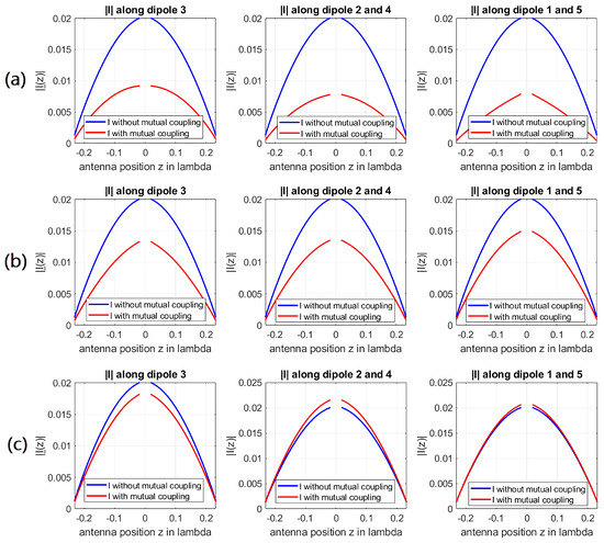
Figure 14.
The current distribution along the different dipoles for the array with (a) spacing, (b) spacing, and (c) spacing between each element. For the blue curve, each element has been computed separately, hence mutual coupling effects were not considered. For the red curve, the elements have been computed as an array; consequently, mutual coupling effects have been considered.
Figure 15 shows the impedance differences between the two methodologies of computing the array for each dipole. At a distance smaller than , where the reactive NF regions of the elements are overlapping, a significant impact on the impedance due to coupling effects can be seen. Above the distance of , still, a deviation is observable due to radiative coupling effects, as the elements are inside the main lobe of the directivity of the other elements. Finally, at an element distance of more than , a maximum at multiples of half the wavelength can be seen, which can be explained by resonance effects that occur between the elements.
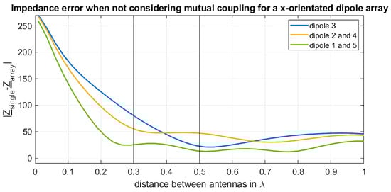
Figure 15.
The difference of the impedance between the two computation methods for every dipole as a function of the distance between the array elements in x-direction.
In contrast to the above-presented results, in Figure 16, the array elements are placed along the z-axis. As can be seen in Figure 12b, in the z-direction, the reactive NF region has a smaller distance to the antenna. Hence, the coupling effects are also decaying faster than in the other case. The overall coupling effect is also much less than in the other case, as each elements are inside a null of the directivity pattern of each element. Hence, with this setting, only reactive coupling can be observed.
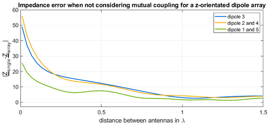
Figure 16.
The difference of the impedance between the two computation methods for every dipole as a function of the distance between the array elements in z-direction.
When again examining the overlapping of the reactive NF regions of the single elements in Figure 13, it can be seen that with the exact knowledge of the surface description of the NF boundary, the coupling behavior between the single elements can be qualitatively predicted. Hence, the introduced surface description is advantageous compared to the radius description.
4. Loop Antennas and the Coupling Behavior of Large Loop Antennas
The electromagnetic power flow around simple loop antennas is analyzed in this section. The introduced error estimators are applied, and the field regions are investigated. As a practical example, the coupling behavior of an electrically large loop antenna is examined.
4.1. Loop Antennas
This section analyzes the power flow and the proposed error estimators for the field regions of a simple loop antenna in the xy-plane. The overall circumference C of the loop antenna is given with , , and . Hence, electrically short and electrically large loop antennas are presented, which results in non-uniform current distributions for the electrically large loop antenna. The loops are excited at an angle of , with a finite feed-gap of . Hence, effects based on the feed-gap are also considered. Consequently, a symmetry will be seen regarding the xy-plane and the xz-plane. For the Poynting vector visualization, the vectors are plotted at a random seed of points; hence, non-symmetric behavior in the quiver-plots is only due to visualization reasons.
In Figure 17, the real part and the imaginary part of the Poynting vector in the coordinate planes around a loop antenna are shown. As seen in the xy-plane in Figure 17a, the real part of the Poynting vector also has non-radial parts. Hence, a transition zone can be observed. For higher distances to the antenna origin, these non-radial components vanish, and a rotationally symmetrical behavior can be observed in the xy-plane. In the xz-plane in Figure 17c, a net power flow in the -direction around the antenna can be seen. This power flow is directed from the direction to the direction. Again, this non-radial net power flow vanishes at higher distances, and pure radial components can be seen. The same occurs for the magnetic dipole; for the angles and , the real part of the energy flow vanishes at higher distances. Consequently, a donut-shaped directivity pattern can be expected.
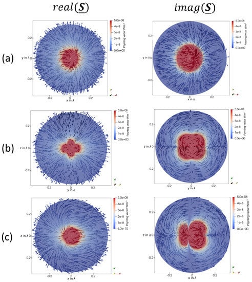
Figure 17.
(a) The real and imaginary part of the Poynting vector in the xy-plane of a loop antenna with an overall circumference of . (b) The real and imaginary part of the Poynting vector in the yz-plane of a loop antenna with an overall circumference of . (c) The real and imaginary part of the Poynting vector in the zx-plane of a loop antenna with an overall circumference of .
When investigating the imaginary part of the Poynting vector in the yz-plane, shown in Figure 17b, it can be seen that there is a fluctuating power flow in the four quadrants of this plane between the directions , , and the direction . As for small dipoles, the shape of the magnitude of the imaginary part of the Poynting vector forms a kidney shape. In the xz-plane in Figure 17c, two separate regions with a dominant imaginary part of the Poynting vector can be seen, with a null in between. This behavior can be explained as a combination of the loop’s inductive behavior and the feeding point’s capacitive behavior.
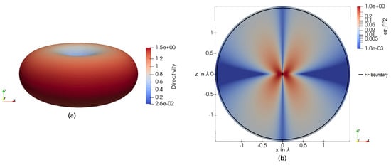
Figure 18 shows the directivity (a) and the FF error-estimator 6 in the xy-plane (b), yz-plane (c), and zx-plane (d) for a loop antenna with the circumference of . Again, it can be observed that the highest FF error is present between nulls and lobes of the directivity pattern. Hence, a quite-low error can be seen in the xy-plane, where the main lobe is present. At the FF boundary for small antennas , the error decreased to about 0.01. Following this, the FF boundary proposed from the literature can be used without any restrictions. The maximum directivity is the same as for a magnetic dipole as well as for a Hertzian dipole. Additionally, the directivity pattern behaves the same as for small dipole antennas.
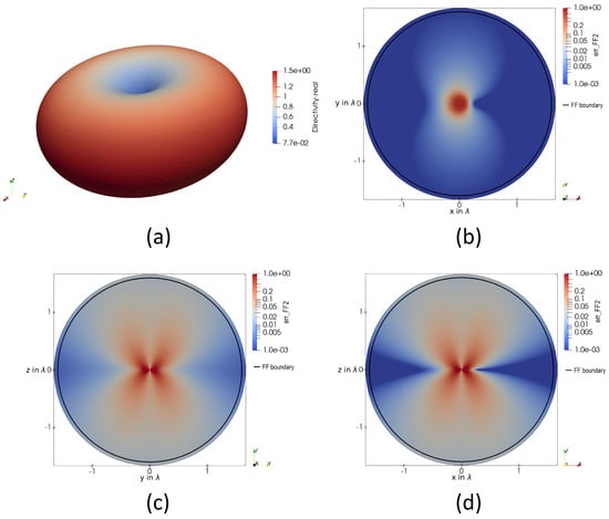
Figure 18.
(a) A 3D plot of the directivity of a loop antenna with the circumference of . The error-estimator 6, describing a qualitative measure of the FF quality, applied on a loop antenna with the circumference of in the (b) xy-plane, (c) yz-plane, and (d) zx-plane. The FF boundary for the given antenna dimension given in 4 is displayed as a black circle.
In Figure 19, the real and the imaginary part of the Poynting vector in the coordinate planes around a loop antenna are shown. Compared to the loop antenna with a circumference of in Figure 17, barely any differences can be seen. This can be explained as the loop antenna is the border case for being electrically small. However, similar field behavior is still observable, as for the electrically very small antenna. For the real part, barely no difference can be seen. As a consequence, the directivity has to also behave the same. When comparing the imaginary part of the power flow, it can be seen that in the xz-plane in Figure 17c, the second reactive region at increased. This can be explained due to the not-uniform current distribution along the antenna structure. As for very small loop antennas, in the yz plane Figure 17b, a kidney-shaped behavior of the magnitude of the imaginary part of the Poynting vector can be seen.
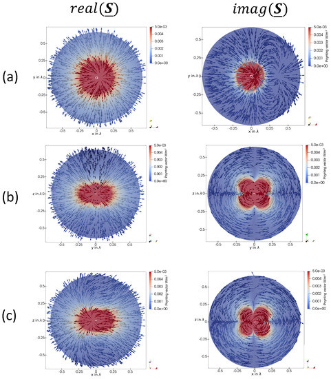
Figure 19.
(a) The real and imaginary part of the Poynting vector in the xy-plane of a loop antenna with an overall circumference of . (b) The real and imaginary part of the Poynting vector in the yz-plane of a loop antenna with an overall circumference of . (c) The real and imaginary part of the Poynting vector in the zx-plane of a loop antenna with an overall circumference of . In each sub-figure, the loop antenna is indicated as a white circle.
Figure 20 shows the directivity (a) and the FF error-estimator 6 in the xy-plane (b), yz-plane (c), and zx-plane (d) for a loop antenna with the circumference of . No difference can be observed compared to the loop antenna qualitatively. As a circumference of can still be seen as electrically short, the directivity pattern and the maximum directivity are the same.
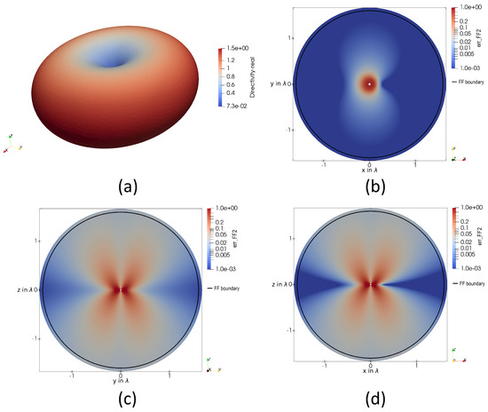
Figure 20.
(a) A 3D plot of the directivity of a loop antenna with the circumference of . The error-estimator 6, describing a qualitative measure of the FF quality, applied on a loop antenna with the circumference of in the (b) xy-plane, (c) yz-plane, and (d) zx-plane. The FF boundary for the given antenna dimension given in 4 is displayed as a black circle.
In Figure 21, the real and the imaginary part of the Poynting vector in the coordinate planes around a loop antenna are shown. For the real part of the Poynting vector, the most significant difference can be observed in the yz-plane in Figure 21b, as the behavior changes and the net power flow in the y-direction decreases faster than in the z-direction, other than for smaller loop antennas. As for larger distances, the net power flow in the y-direction decreases, and the directivity pattern also has to change, compared to small loop antennas.
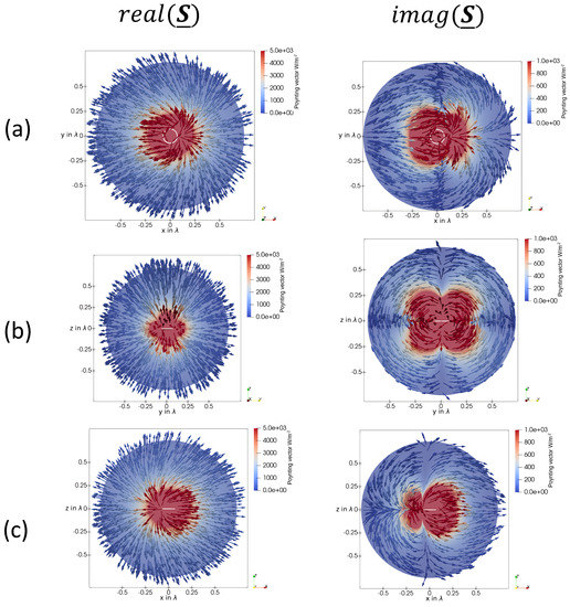
Figure 21.
(a) The real and imaginary part of the Poynting vector in the xy-plane of a loop antenna with an overall circumference of . (b) The real and imaginary part of the Poynting vector in the yz-plane of a loop antenna with an overall circumference of . (c) The real and imaginary part of the Poynting vector in the zx-plane of a loop antenna with an overall circumference of . In each sub-figure, the loop antenna is indicated as a white circle.
A more significant change can be observed for the imaginary part of the Poynting vector. In the xy-plane in Figure 21a, it can be seen that the high-reactive regions are not circular-shaped anymore. This is due to the nonuniform current distribution on the electrically large antenna. For a loop antenna with a circumference of about half a wavelength, on the exciting point at , a voltage maximum is located, and on the other side at , a current maximum. Hence, two separate high-reactive regions exist, a capacitive region at around and an inductive region at around . This can be explained by transmission-line theory, as for , a voltage-maximum and for , a current-maximum is present. Additionally, the behavior in the xz-plane in Figure 21c changed, caused by the same reason.
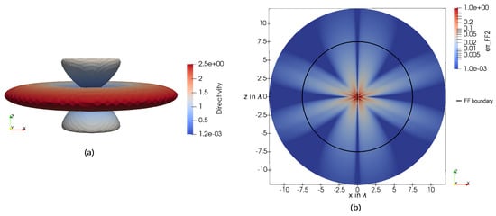
Figure 22 shows the directivity (a) and the FF error-estimator 6 in the xy-plane (b), yz-plane (c), and zx-plane (d) for a loop antenna with the circumference of . The directivity in Figure 22a differs essentially from an electrically short dipole. The power flow shifted from the y-direction towards the z-direction. Additionally, no null in the directivity pattern is observable. The maxima are located in the positive and negative x-direction. Hence, an almost rotationally symmetrical behavior along the x-axis can be seen. The xy-plane and xz-plane of the error-estimator 6 behave qualitatively the same. In Figure 22c, it can be seen that the maximum error lies in the yz-plane. As for smaller loop antennas or dipole antennas, this is again between two maxima of the directivity pattern. At the FF boundary for small antennas , the error decreased to about 0.01. Hence, the proposed FF boundary can be seen as reliable.
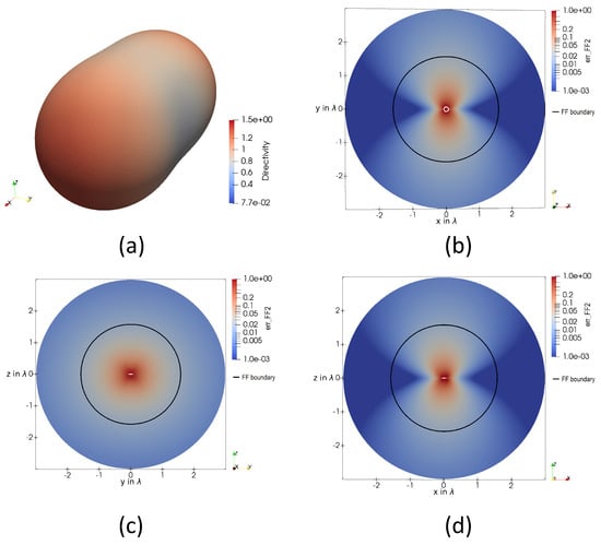
Figure 22.
(a) A 3D plot of the directivity of a loop antenna with the circumference of . The error-estimator 6, describing a qualitative measure of the FF quality, applied on a loop antenna with the circumference of in the (b) xy-plane, (c) yz-plane, and (d) zx-plane. The FF boundary for the given antenna dimension given in 4 is displayed as a black circle. The loop itself is given as a white circle.
In Figure 23, the proposed reactive NF region is shown for loop antennas with the circumference (a) , (b) , (c) , and (d) . The regions have been derived with the error estimator 11, postulating . Hence, the oscillating power flow normal to the enclosing surface equals the time-averaged power flow.
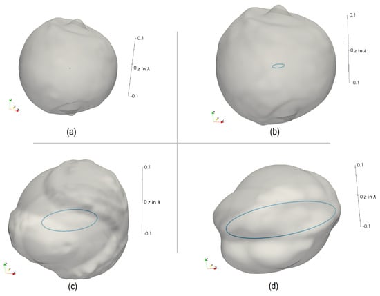
Figure 23.
The reactive NF region, described by the angular-dependent radius , when applying the error estimator 11 with of a loop antenna with the circumference of (a) , (b) , (c) , and (d) .
By investigating Figure 23 in detail, it can be seen that the reactive NF region of electrically small loop antennas in (a) and (b) have an almost spherical structure with a radius of . For the loop antenna with a circumference of , a toroidal-like behavior with a bulge at the positive and negative z-axis can be observed. Nevertheless, a sphere can still be seen as a good approximation.
Two main regions can be observed when the loop antenna is electrically large, as for the loop antenna in Figure 23c. One region is around the xy-plane between and for negative x-values. Here, a current maximum on the conducting structure occurs, and following, mainly inductive behavior can be expected. The second region can be seen from to for . As for , the voltage maximum can be observed. This region can be seen as highly capacitive. Still, the overall reactive NF region can be approximated by a sphere with the radius .
Figure 23d shows a loop antenna. As can be seen, a sphere cannot approximate the reactive NF region for electrically large antennas bigger than half a wavelength. For this type of antenna, mainly a toroid-shape behavior around the conducting structure can be seen. At the position where current or voltage maximums occur, the reactive NF region is more pronounced.
4.2. Coupling Behavior of an Electrically Large Loop Antenna
This section analyzes the coupling behavior of a loop antenna with the circumference of . Therefore, first, the reactive NF region is examined in more detail. Second, an electrically small dipole antenna (the coupling mechanism is mainly capacitive) and an electrically small loop antenna (the coupling mechanism is mainly inductive) are placed near the antenna and the induced voltage is analyzed.
In Figure 24, the reactive NF region of a loop antenna is shown. Two main regions can be observed: one with a negative imaginary part of the normal component of the Poynting vector (blue) and one with a positive imaginary part (red). As the blue region is close to the current maximum on the current structure, higher inductive coupling behavior can be expected. The red region is close to a potential maximum—consequently, higher capacitive coupling behavior can be expected.
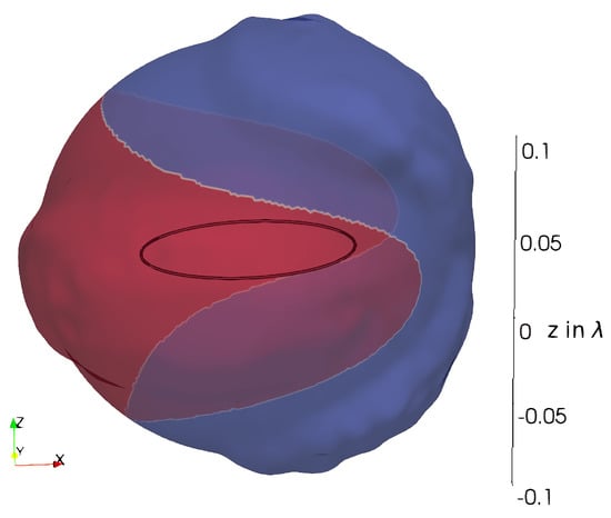
Figure 24.
The reactive NF region of a loop antenna with the circumference of , determined by applying the error-estimator in 11, is given. The red surface shows the region where the imaginary part of the normal component of the Poynting vector is positive, and the blue surface shows the region with a negative imaginary part.
Figure 25 shows the simulation setup to analyze the coupling behavior. Here, the analyzed loop antenna is excited. Then, an additional electrically small, open-circuited loop antenna is placed above the excited loop to sense the inductive coupling. In the second setup, an electrically small dipole antenna is placed above the excited loop antenna, to mainly sense the capacitive coupling.
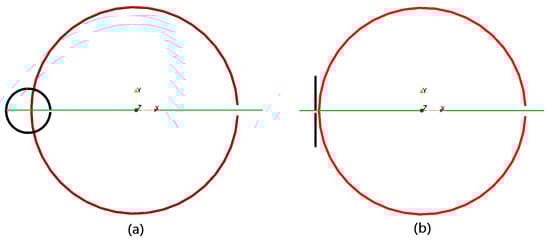
Figure 25.
Simulation setup for the coupling investigations. For both setups, a loop antenna (red) is placed in the xy-plane. The feed-gap is placed in the -direction. In (a), an electrically small loop antenna is placed parallel to the big loop with a z-distance of . In (b), a y-orientated electrically small dipole antenna is placed above the big loop antenna, with a z-distance of . The small loop (a) and small dipole (b) are placed along the green line to analyze the coupling behavior for different points.
In Figure 26, the induced voltage on the loop probe (a) and dipole probe (b) are shown. As seen in the loop probe, the maximum of the induced voltage can be observed for negative x-values. As already discussed, this area is mainly inductive. The following behavior could be expected. Around the feed-gap of the excited loop, mainly capacitive behavior is expected. Hence, also the induced voltage on the loop probe is significantly smaller. Additionally, two positions with a voltage minimum can be observed. These minima occur as at these positions, half of the probe loop’s area overlaps the inside of the excited loop, and the other half of the area is outside the excited loop. Hence, the magnetic flux cancels, which is called zero-coupling behavior.
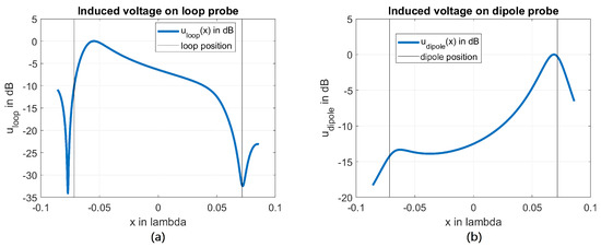
Figure 26.
The induced voltage of a loop probe (a) and a dipole probe (b) when moved along the green line denoted in Figure 25 above a loop antenna.
For the dipole probe, inverse behavior can be observed. Here, the maximum is given above the feed-gap of the excited loop. This behavior can be explained, as the voltage along the conducting structure is maximized at this position. Additionally, the highest capacitive coupling behavior can be observed. At negative x-values, the excited loop has a voltage minimum and shows mainly inductive behavior. Hence, the capacitive coupling is minor.
Therefore, by introducing the surface-based NF boundary and categorizing the surface, using the sign of the imaginary part of the Poynting vector, advanced predictions regarding the coupling behavior can be given.
5. Conclusions
The field regions around simple antenna structures are analyzed using a Poynting vector-based approach. A new method for defining the reactive NF region using an arbitrary surface instead of a radius is introduced. Finally, the main findings are applied to practical examples to predict the coupling behavior of neighboring radiating structures.
It was shown that the introduced error-estimators give a valuable measure to analyze the field behavior in the different field regions defined by the IEEE-standard [1].
When analyzing simple dipole and loop antennas, it could be shown that the FF boundary proposed in the literature can be used as a good approximation. The most significant directivity error is made between maxima and minima in the directivity pattern. There, radiating energy flows into the lobes, present in the FF directivity pattern. By visualizing the real part of the complex Poynting vector, the transition zone, as well as the formation of the directivity pattern, can be observed.
By analyzing the boundary between the reactive and radiating NF, it could be seen that a simple radius is insufficient for electrically large antennas to define the reactive NF region. Consequently, an angular-dependent radius has been proposed to border this region. The benefit of the introduced reactive NF region has been examined by analyzing the coupling behavior of a linear antenna array. There, we could show that the coupling behavior could be predicted with the knowledge of the defined field region boundaries. The enveloping surface of the reactive NF region can further be classified by the sign of the imaginary part of the Poynting vector. In doing so, it could be shown that the inductive or capacitive coupling behavior can be predicted with the detailed knowledge of the field regions.
Author Contributions
Conceptualization, P.B. and T.B.; methodology, P.B.; software, P.B. and A.M.; formal analysis, P.B.; investigation, A.M., P.B. and C.R.; writing—original draft preparation, P.B.; writing—review and editing, P.B., T.B. and A.M.; visualization, A.M.; supervision, T.B. All authors have read and agreed to the published version of the manuscript.
Funding
This research received no external funding.
Acknowledgments
The authors want to thank Riccardo Torchio from the University of Padua for providing his PEEC toolbox. The solver can be accessed via [14].
Conflicts of Interest
The authors declare no conflict of interest.
Abbreviations
The following abbreviations are used in this manuscript:
| NF | Near-field |
| FF | Far-field |
| PEEC | Partial element equivalent circuit |
| EMI | Electromagnetic interference |
References
- IEEE. IEEE Standard for Definitions of Terms for Antennas. In IEEE Std 145-2013 (Revision of IEEE Std 145-1993); IEEE: Piscataway, NJ, USA, 2014; pp. 1–50. [Google Scholar] [CrossRef]
- Paul, C.R. Introduction to Electromagnetic Compatibility (Wiley Series in Microwave and Optical Engineering); Wiley-Interscience: Hoboken, NJ, USA, 2006. [Google Scholar]
- Li, H.; Khilkevich, V.V.; Pommerenke, D. Identification and Visualization of Coupling Paths—Part I: Energy Parcel and Its Trajectory. IEEE Trans. Electromagn. Compat. 2014, 56, 622–629. [Google Scholar] [CrossRef]
- Li, H.; Khilkevich, V.V.; Pommerenke, D. Identification and Visualization of Coupling Paths—Part II: Practical Application. IEEE Trans. Electromagn. Compat. 2014, 56, 630–637. [Google Scholar] [CrossRef]
- Baumgartner, P.; Bauernfeind, T.; Renhart, W.; Biro, O.; Torchio, R. Limitations of the Pattern Multiplication Technique for Uniformly Spaced Linear Antenna Arrays. In Proceedings of the 2016 International Conference on Broadband Communications for Next Generation Networks and Multimedia Applications (CoBCom), Graz, Austria, 14–16 September 2016. [Google Scholar]
- Stutzman, W.; Thiele, G. Antenna Theory and Design, 3rd ed.; Wiley: Hoboken, NJ, USA, 2012. [Google Scholar]
- Laybros, S.; Combes, P. On radiating-zone boundaries of short, /spl lambda//2, and /spl lambda/ dipoles. IEEE Antennas Propag. Mag. 2004, 46, 53–64. [Google Scholar] [CrossRef]
- Amin, S.; Ahmed, B.; Amin, M.; Abbasi, M.I.; Elahi, A.; Aftab, U. Establishment of boundaries for near-field, fresnel and Fraunhofer-field regions. In Proceedings of the 2017 IEEE Asia Pacific Microwave Conference (APMC), Kuala Lumpur, Malaysia, 13–16 November 2017; pp. 57–60. [Google Scholar] [CrossRef]
- Vallauri, R.; Bertin, G.; Piovano, B.; Gianola, P. Electromagnetic Field Zones Around an Antenna for Human Exposure Assessment: Evaluation of the human exposure to EMFs. IEEE Antennas Propag. Mag. 2015, 57, 53–63. [Google Scholar] [CrossRef]
- Baumgartner, P.; Bauernfeind, T.; Renhart, W.; Biro, O. Numerical Investigations of the Field Regions for Wire Based Antenna Systems. IEEE Trans. Magn. 2019, 56, 7513204. [Google Scholar] [CrossRef]
- Ruehli, A.; Antonini, G.; Jiang, L. Circuit Oriented Electromagnetic Modeling Using the Peec Techniques; John Wiley & Sons, Ltd.: Hoboken, NJ, USA, 2017; Volume 1. [Google Scholar]
- Jackson, J.D. Classical Electrodynamics, 3rd ed.; Wiley: New York, NY, USA, 1998. [Google Scholar]
- Balanis, C.A. Antenna Theory: Analysis and Design; Wiley-Interscience: Hoboken, NJ, USA, 2005. [Google Scholar]
- Torchio, R. Github Riccardo Torchio. 2022. Available online: https://github.com/UniPD-DII-ETCOMP?tab=repositories (accessed on 16 May 2022).
Publisher’s Note: MDPI stays neutral with regard to jurisdictional claims in published maps and institutional affiliations. |
© 2022 by the authors. Licensee MDPI, Basel, Switzerland. This article is an open access article distributed under the terms and conditions of the Creative Commons Attribution (CC BY) license (https://creativecommons.org/licenses/by/4.0/).