Abstract
In this paper, battery electric vehicle (BEV) controllers are smartly tuned with particle swarm optimization (PSO) and genetic algorithm (GA) to ensure good speed regulation. Intelligent tuning is ensured with a proposed and well-defined cost function that aims to satisfy the design requirements in terms of minimum overshoot, fast response, and tolerable steady state input. Two proposed cost functions are formulated for both simple speed input and for driving cycles. The BEV is controlled with the field oriented control technique (FOC), and it is driven by a permanent magnet synchronous motor (PMSM). An efficient control scheme based on FOC is built using a simplified closed loop control system including BEV components such as regulators, inverter, traction machine, and sensors. Simulation results show that the optimum controller gains obtained by intelligent tuning have resulted in satisfactory BEV performance that sustains the harsh environmental conditions. Robustness tests against BEV parameter changes and environmental parameter variations confirmed the effectiveness of intelligent tuning methods.
1. Introduction
Today, one trend in the field of electrical engineering is the integration of renewable energy sources in almost all engineering disciplines [1,2,3,4]. For instance, wind, solar, and tidal energies, which are clean and renewable sources, have successfully replaced the conventional methods of electricity production. In the field of automotive engineering, conventional vehicles that rely on the use of exhaustible and polluting energy sources are being continuously substituted with HEV [5,6,7]. Being ecologically and environmentally friendly, electric vehicles have gained traction in the market and have pushed many countries around the world to reorient their policies toward the electrification of their transport sectors already suffering from greenhouse gas emissions. Figure 1 shows that Global HEV sales reached 6.75 million units in 2021, 108% more than in 2020. This volume includes passenger vehicles, light trucks, and light commercial vehicles [8]. The remarkable growth rate of 108% is relative to the low base volume of 2020 mainly caused by regulations and COVID-19, global HEV sales of 2019 and 2020 were below the long-term trajectory, and in 2021 they returned back to trend, as it can be seen in Figure 1.
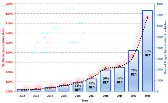
Figure 1.
Global electric vehicle sales.
Over the past few years, a lot of research has been carried out to investigate various aspects of the development of sustainable low-carbon transportation technologies to solve the persistent problem of carbon emissions. Vehicle electrification is an efficient solution for reducing or totally eliminating gas emissions. This fact has significantly challenged researchers to explore new research axes and to propose new solutions toward the elaboration of an efficient and ecological vehicle. Control of electric propulsion systems [9,10,11], intelligent energy management [12,13,14], intelligent transportation and vehicular communication systems [15,16,17], autonomous vehicles [18], vehicle chassis systems [19], power electronics [20], power train architecture [21], vehicle safety [22], and machine control [23] are among the biggest current trends in automotive engineering. Driveline architecture is a key factor for improving the performance of HEVs. For this reason, it has been widely diversified since the invention of HEVs. The number and the location of the used electric machines is used as a scale in HEV classification. Information about HEV classifications is detailed in [24].
Electrical vehicles are subjected to different driving cycles, which are used to predict the behavior and the performance of electric drive systems. Some of these driving cycles are derived theoretically, as it is preferred in the European Union, whereas others are derived from direct measurements. More information about driving cycles is discussed in detail in [25]. A driving cycle is a set of data representing an HEV speed over time. The collected data reflect the driver’s behavior in different driving situations (e.g., city, highway). These cycles are used for measuring different HEV performances such as battery, fuel consumption minimization, and HEV road side performance. Table 1 summarizes different driving cycles classifications found in the literature.

Table 1.
Different driving cycle classifications.
A permanent magnet synchronous motor (PMSM) is a machine which uses permanent magnets instead of electromagnets in order to produce the air gap magnetic fields [26]. In recent years, especially in the last decade, permanent magnet synchronous motor (PMSM) drives have been extensively employed in various domains, such as wind-power generation and traction applications, especially electric vehicles. PMSM has several advantages over other machines such as its high efficiency, high torque and power-to-inertia ratios, and high acceleration and deceleration rates [27]. During the last decade, more attention was given to optimization techniques and researchers still try to inspire new optimization algorithms from natural wisdom. These new emerging optimization techniques such as the genetic algorithm (GA), convex optimization, the particle swarm optimization (PSO) algorithm, the biogeography algorithm, the brain emotional learning algorithm, and their modified versions are extensively used in different fields due to their simplicity, effectiveness, and quickness in comparison with other classical methods, which are tedious and time consuming. These naturally inspired algorithms mentioned so far find many applications. One of the most used application area of these algorithms is the control of drive systems. In [28], the convex optimization algorithm is used to optimize the performances (speed) of the permanent magnet synchronous motor (PMSM) drive system. However, in [29], the genetic algorithm (GA) is used to regulate the speed of a permanent magnet synchronous motor. In [30], authors have used the biogeography optimization algorithm for an optimal adjustment of the Proportional Integral (PI) parameters for the speed regulation of a permanent magnet synchronous motor (PMSM). In [31], the brain emotional learning algorithm is used for PI tuning of a permanent magnet synchronous machine (PMSM) drive. In [32], the authors have used particle swarm optimization (PSO) to automatically tune the PI controller for speed regulation of a PMSM. Artificial intelligence techniques are extensively used in the field of hybrid electric vehicles [33]. In [34], the authors have developed an effective energy management strategy under different driving cycles, and they have found that the optimized fuzzy logic strategy is better in terms of energy-saving compared to other techniques used. In [35], the authors have developed a heuristically learning- charging cost optimization algorithm (CCOA) for the residential charging of electric vehicles. In [36], the authors have used a metaheuristic-based vector-decoupled algorithm to balance the control and operation of hybrid microgrids in the presence of stochastic renewable energy sources and an electric-vehicle charging structure. In [37], an adaptive equivalent consumption minimization strategy based on a recurrent neural network is presented to solve the multi-objective optimal control problem for a plug-in hybrid electric vehicle. In [38,39,40], the authors propose particle swarm optimization as a method for controlling power-split hybrid electric vehicles within ≥an optimized fuel economy. In this paper, particle swarm optimization and genetic algorithms with a new proposed cost function are used for speed regulation by properly adjusting the PI parameters of the speed and current controllers.
The authors in [41] have designed a robust speed controller for a hybrid electric vehicle, and they use fractional order PID; however, the designed controller and its robustness were tested only for simple and custom speed profiles that bear little resemblance to the real speed profiles to which the electric vehicle is subjected in real situations. The authors in [42] have discussed an adaptive fault tolerant control of an electrical vehicle, but they did not consider driving cycles in any of their simulations, which were restricted to only a few seconds. A novel technique for tuning PI-controllers is proposed in [43] and a reliable speed controller for electrical vehicles was designed in [44]; in these two last mentioned works, authors have considered that the control of an electric vehicle comes back to the control of the traction machine whose speed reference and load torque are just simple step inputs neglecting the fact that the BEV is in reality subjected to driving cycles and load torque, which are variable and much more complex than a simple step input. In [45], the authors have taken into consideration driving cycles when analyzing the performance of a permanent magnet synchronous motor used in a vehicle’s traction, but they have neglected some important external parameters that affect vehicle performances, such as wind; moreover, authors in that article have considered a constant rolling resistance during all of the driving cycle periods, neglecting the fact that the rolling resistance depends on several parameters, such as vehicle speed, ground surface, and tire inflation, which are not consistent across the path traveled by the vehicle.
In this work, intelligent optimization algorithms (PSO/GA) are used to optimize the parameters of the speed controller of the electric vehicle. This is done through a proposed and simplified control scheme that considers the real load conditions to which the BEV is subjected. The BEV is controlled with the field-oriented control technique, and the PI controllers used for BEV speed and PMSM current control are tuned with classic and intelligent control techniques. The PMSM used to ensure BEV traction is subjected to variable load torque conditions that depend on BEV speed and on environmental conditions. The rolling-resistance coefficient is considered to be variable depending on vehicle speed. Robustness tests were performed to see whether the BEV control system performs well in case of variations of some of its parameters and the variations of environmental parameters.
2. Vehicle Dynamics
When a vehicle is undergoing a given driving cycle, it is subjected to some external forces, which tend to attenuate or to amplify its speed. The motion of the vehicle shown in Figure 2 is governed by the following equation:
is the net external force acting on the vehicle body, is the vehicle mass, and is the vehicle acceleration.
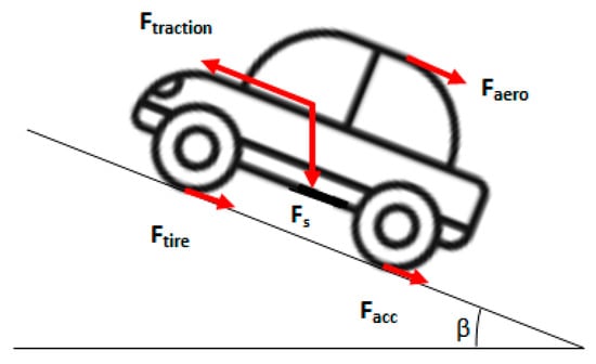
Figure 2.
Forces exerted on the vehicle.
Equation (1) can be rewritten as highlighted with Equation (2):
where is the net resistive force acting on the BEV. It is defined as given in Equation (3):
is the aerodynamic force, is the force due to road slope, and is the force due to friction between vehicle tires and ground surface.
2.1. Aerodynamic Force
The vehicle encounters air resistance while it travels, and this phenomenon is called aerodynamic drag. This force is modeled by the mathematical expression given by Equation (4):
where ρ is the air density (kg/m3). A is the vehicle frontal area (m2), is the aerodynamic drag coefficient (s2/m2), is the vehicle longitudinal speed (m/s), and is the wind speed (m/s).
2.2. Slope Force
This force is due to road inclination, and it is proportional to the mass of the vehicle. It is given by Equation (5), where g is the gravity acceleration (m/s2) and is the road inclination angle (radians).
2.3. Rolling Force
This force is due to the friction between a vehicle’s tires and the ground surface. It depends on several parameters, such as pressure, tire deflection, ground surface, which may be hard or soft and vehicle speed. The rolling-resistance force is given by Equation (6) shown below:
is the rolling-resistance coefficient. Typical values of the rolling-resistance coefficient are provided in Table 2.
Table 2.
Rolling-resistance values for different road types.
In fact, the values provided in Table 2 do not consider the variations of with respect to speed. In this work, the rolling resistance is related to vehicle velocity with the linear relation given in Equation (7) that predicts the values of the rolling-resistance constant with acceptable accuracy for speeds up to 128 km/h [46]:
2.4. Acceleration Force
Acceleration force names the necessary force needed to accelerate from zero to maximum speed. It is given by the Equation (8) shown below:
is the maximum vehicle speed (m/s), g is the gravity acceleration, and is the time characteristic of the vehicle (s).
All cars have gears, including electric cars. However, most electric cars neither have nor need a multispeed transmission due to the high torque available over a very wide range of motor speeds and because electric motors produce their peak torque at 0 rpm. Generally, the electric motor is always connected to the drive wheels through a simple gear with a fixed ratio. Speed and torque on a motor’s shaft are not the same on a vehicle’s wheels. The torque (Tm) and the mechanical speed () transmitted from the motor’s shaft (Tm) to the driven wheels are respectively given by Equations (9) and (10):
is the total gear ratio of the driveline and is the driveline efficiency of a motor’s shaft in relation to the driven wheels. The electric vehicle used in this paper is under the name of “Microlino”, and all its parameters are provided in Table 3. In this work, the permanent magnet synchronous machine (PMSM) is responsible for vehicle traction. Hence, the PMSM should be able to sustain the maximum load torque applied on it. From Table 2, the PMSM can handle a maximum torque of 111 N·m and the Microlino electric vehicle can develop a maximum torque of 110 N·m as it is highlighted in Table 3. To summarize, the Microlino electric vehicle was chosen because it develops a maximum torque that is in the range of the nominal values that can be sustained by the traction machine (PMSM).
Table 3.
Electric vehicle and environmental parameters.
3. PMSM Model
Permanent magnet synchronous motors present higher efficiency, a high torque-to-mass ratio, and competitive dynamic performance compared to asynchronous motors without sacrificing reliability. It has also been shown that these motors can be operated over a wide constant power speed range [47]. In this section, the modeling and analysis of the permanent magnet synchronous machine is carried out in both time and frequency domain.
Stator voltage is expressed by Equation (11) shown below:
Stator flux in both direct and quadrature axes is expressed by Equation (12):
where rs is the stator resistance, id is the d-axis stator current, iq is the q-axis stator current, λd is the d-axis flux linkage, λq is the q-axis stator flux linkage. Ld is the d-axis inductance, Lq is the q-axis inductance, and is the flux linkage due permanent magnets. We is the electrical speed, and wr is the motor mechanical speed. For a machine with p pair of poles, electrical and mechanical speed are related by the following formula:
Importing Equations (12) and (13) into Equation (11) yields Equation (14):
Converting the two last equations to Laplace domain yields:
The electromagnetic torque developed by the PMSM is given by the following expression:
It is worth noticing that a rotor’s rotation produces a mechanical torque given by the following equation where represents the electromagnetic torque and is the mechanical load torque.
Equation (17) can be expressed in Laplace domain as follows where is the inertia of the rotor (Kg·m2) and B is the mechanical damping coefficient. The parameters of the PMSM motor used in this work are shown in Table 4:
Table 4.
BEV and environment parameters.
4. FOC Control of Electric Vehicle
AC machine control is a difficult task due to several reasons like the nonlinearity of the machine model and the strong coupling and interaction that exists between stator and rotor fields. The idea behind field oriented control is to always keep the stator field perpendicular to the rotating rotor field as it is shown in the Figure 3. It is worth noticing that represents the stator flux reference represents the measured stator flux.
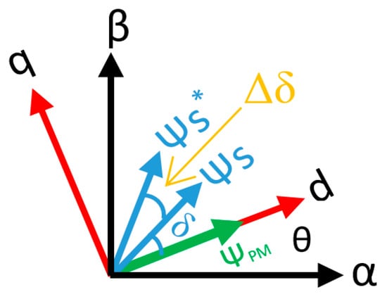
Figure 3.
Stator and rotor field orientations in dq axis.
Today, several control techniques are used for the control of PMSM such as direct torque control (DTC) and field-oriented control. This last control technique is used for obtaining large instantaneous speed regulation without developing current and torque ripples for low speeds, as it is the case in DTC. Figure 4 shows a general scheme of field-oriented control technique applied to the BEV. A current feedback loop is formed by sensing then transforming the stator phase currents to a coordinate system rotating with the rotor of the machine. Vehicle speed is also measured and then compared with its reference forming a speed loop. This speed error is fed into a PID controller, which generates the reference torque. Setting the d-axis current to zero in Equation (16) maximizes the electromagnetic torque of the PMSM and provides the following linear relationship between stator current and motor torque:
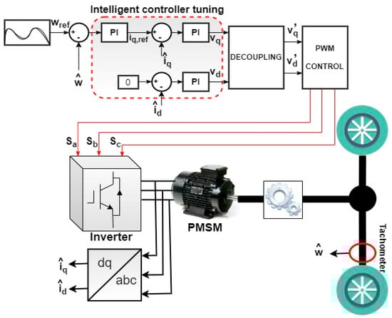
Figure 4.
Electric vehicle field oriented controlled scheme.
One can see that the control of vehicle torque comes back to the control of the q-axis component of the stator current. The inputs to the decoupling block shown in Figure 4 are given by Equation (20) where a strong coupling between direct and quadrature axes can be noticed. The decoupling by compensation approach procedure is used as it is shown in the following equation:
Equating Equations (15) and (20) yields a decoupled system given by the following equations:
The decoupling ensured by Equation (21) enables us to separately analyze the performances of the BEV in direct and quadrature axes. Based on Equations (18) and (19), and (21), a control system model of a BEV driven by PMSM is derived, and it is shown in Figure 5. The outer loop of decoupled control scheme shown in Figure 5 is used to control the speed of the electric vehicle, whereas the inner loop highlighted with red dashed lines is used to control the permanent magnet synchronous currents. It is worth noticing that represents the reference current in the quadratic axis.
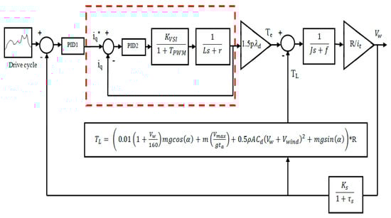
Figure 5.
Decoupled control scheme of the electric vehicle driven by PMSM.
Each stage of the figure above is discussed in detail, as it will be shown below.
4.1. Inverter Model
The output of the decoupling block is supplied to a the three-phase SPWM inverter whose transfer function is given as follows:
where is the inverter gain which is given by:
where is DC voltage input to the inverter and is amplitude of the triangular modulation signal. The inverter time constant is given by the following equation where fm is the frequency of the triangular modulation signal:
4.2. PID Controller Model
PID controllers are used to provide an output whose value is as close as possible to the input reference value with minimum overshoot for a given input. The transfer function of the PID controller shown in Figure 6, which is used in the outer loop for speed and current regulation is given by the following equation:
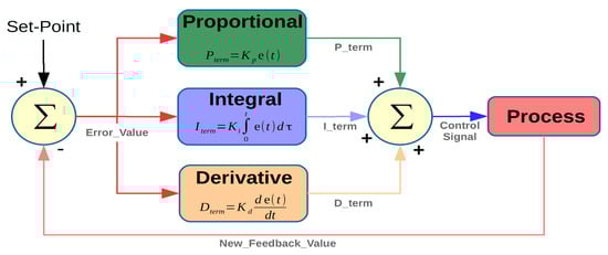
Figure 6.
PID control scheme.
4.3. Sensor Model
A tachometer is used as a tool to calculate a wheel’s speed. This device can be represented by a simple first-order transfer function with a gain KS and time constant Ts and is given by:
In electrical engineering or more precisely in drive control, PMSM speed regulation is usually ensured by PI controllers. Finding those optimum controller parameters is too time consuming, and it is also a risky task, since some the PI gains may damage the system or make it unstable. To overcome these problems, PI gains should be automatically adjusted using the idea that only the best proportional and integral gains should be provided to the PI controller at each instant. This is usually performed using population-based optimization algorithms such as particle swarm optimization (PSO) or genetic algorithm (GA). These two aforementioned naturally inspired algorithms have been used in this work to tune the PI speed controller and optimize its parameters as it will be discussed in the forthcoming section.
5. Intelligent Controllers’ Tuning
5.1. Particle Swarm Optimization
Particle swarm optimization is a population-based algorithm inspired by the social behavior of organisms such as birds and fishes. It was first introduced by Eberhart and Kennedy in 1995. It is similar to other population-based algorithms like (GA) in that the algorithm is initialized with a population of random solutions. To optimize the time complexity of the algorithm, the idea of several evaluations at one iteration was adapted, and this means that all the particles in the population are exploring the search space while at the same time attempting to find an optimal location (solution) with respect to a cost function.
For a population of N particles, the personal and global bests are given by:
where and are the personal and global best position of particle i at iteration t.
The particles’ position is updated by:
where:
- : The ith Particle’s velocity at iteration t.
- : The ith Particle’s position at iteration t.
- : Personal best position of particle i.
- : Personal best position of particle i found in [0 t].
- : Acceleration factors. The relation between c1 and c2 is given by Equation (30):
- : Random coefficients.
- is linearly decreasing [0.4, 0.9].
All the particles’ updated position is given by:
Table 5 shown below contains all the PSO parameters that have been used when performing the different simulations, and the PSO pseudocode is shown in Figure 7.
Table 5.
PSO parameters.
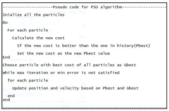
Figure 7.
Pseudo code of PSO algorithm.
5.2. Genetic Algorithm
GA is a stochastic universal adaptive search optimization technique based on the procedure of inherent selection. Darwin also stated that the survival of an organism can be maintained through the process of selection, crossover, and mutation. The solution generated by GA is called a chromosome, while the collection of chromosomes is referred as a population that will undergo a process called evaluation to measure the suitability of a solution. Some chromosomes will mate through a process called crossover, producing offspring that are the combination of their parents’ genes. In a generation, few chromosomes will undergo mutation in their genes. The number of chromosomes that will undergo crossover and mutation is controlled by the crossover rate and the mutation-rate value. The chromosomes that will be maintained for the next generation will be selected based on Darwin’s rule; the chromosome with higher fitness or lower cost value will have greater probability of being selected again in the next generation. After several generations, the chromosome value will converge to a certain value which is the best solution for the problem. Figure 8 shown below points out a GA flowchart, which explains the different major steps of this algorithm.
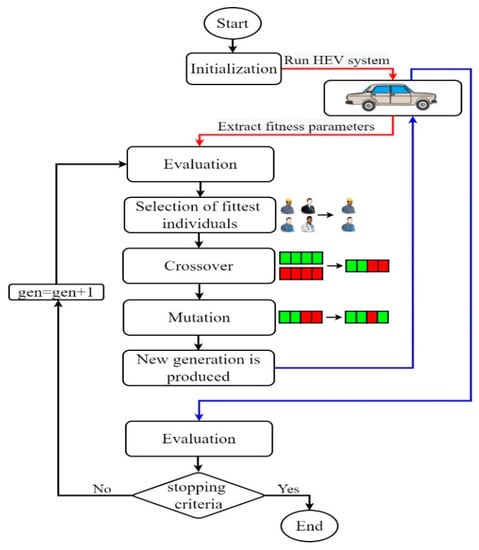
Figure 8.
Genetic algorithm flowchart.
Each step of the algorithm shown below is explained below:
- Search space initialization
In solving problems, some solutions will be the best among others. The space of all feasible solutions (among which the desired solution resides) is called search space. Each point on this state space is a possible solution that is characterized by its cost for the problem. Figure 9 shows a GA population in a four-dimensionional search space. One can remark that the first two dimensions are dedicated to the speed regulator and the last two ones are reserved for the PI current controller.
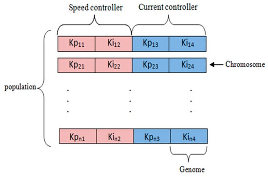
Figure 9.
GA PI controller.
- Selection
Selection names the process of choosing the fittest chromosomes based on their cost. The number of chromosomes selected for crossover is decided by the selection factor. Many techniques exist for selecting chromosomes such as roulette-wheel selection, rank selection, and tournament selection. Roulette-wheel selection, which is the most commonly used technique for chromosome selection, is the technique that has been used in this project; for this reason, we will explain bellow its principle of operation.
- Calculate the cost of each chromosome F(i).
- Calculate the selection probability for each chromosome with Equation (32):
- Compute the cumulative probability values.
- Generate two random vectors, R1 and R2.
- Basing our selection on R1 and R2, we select two sets of chromosomes (parents) for crossover.
In this method, each individual is allocated a section of a roulette wheel. The size of the section is proportional to the cost of the individual. A pointer is spun and the individual to whom it points is selected. This continues until the selection criterion has been met. The probability of an individual being selected is related to its cost, ensuring that fitter individuals are more likely to leave offspring. Figure 10 in the next page illustrates the roulette wheel selection:
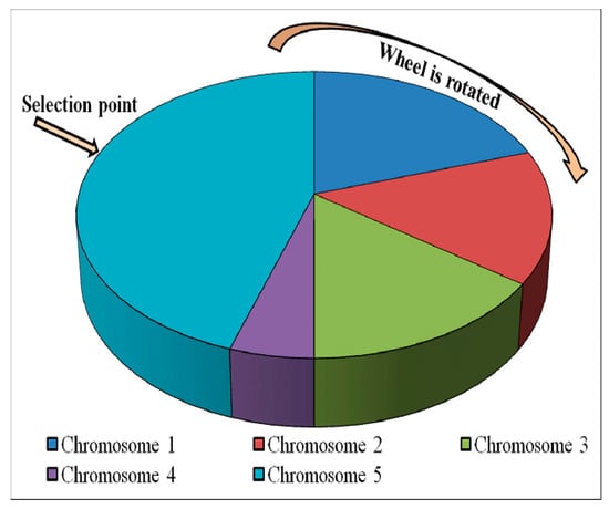
Figure 10.
Depiction of roulette Wheel selection.
- Crossover
Crossover is a genetic operator that combines (mates) two chromosomes (parents) to produce a new chromosome (offspring). The idea behind crossover is that the new chromosome may be better than both of the parents if it takes the best characteristics from each of the parents. There exist two types of crossover: single-point crossover and two-point crossover. When performing a single-point crossover, both parental chromosomes are split at a randomly determined crossover point, and then a new child genotype is created by appending the first part of the first parent with the second part of the second parent. A single crossover point on both parents’ organism strings is selected. All data beyond that point in either organism string is swapped between the two parent organisms. The advantage of having more crossover points is that the search space may be searched more thoroughly. However, adding further crossover points reduces the performance of the GA.
- Mutation
Mutation means the flipping of variable values. For every chromosome, the variable value that will change is randomly selected. Using selection and crossover on their own will generate a large amount of different strings. However, the following problem will be faced when using only selection and crossover; depending on the initial population chosen, there may not be enough diversity in the initial strings to ensure the genetic algorithm searches the entire search space. Furthermore, the genetic algorithm may converge to sub-optimum strings due to a bad choice of initial population. These problems may be overcome by introducing a mutation operator into the genetic algorithm. Table 6 points out all the GA parameters used when performing the different simulations:
Table 6.
GA parameters.
5.3. Cost Function and Performance Assessement
A cost function is a mathematical formula used to measure and evaluate the goodness or the performance of a given particle (potential solution). In most cases, the cost function is constructed from the different parameters that do affect the system output, or it is constructed with some well-defined error functions. In general, four criteria are employed to judge the suitability of the PID parameters. The performance criteria that are mostly used in control system design and summarized as follows:
The performance of our system is measured with a cost function. It is used to provide a measure of how good the solution is and how the potential solutions have performed in the problem domain. A good formulation of the cost function will have a positive impact on the BEV system by enhancing its performances. In this paper, we have considered two types of speed inputs: step-input reference (simple) and driving cycles (complex). For simple speed inputs, one can use system performance indices such as rising time, percentage overshoot, and steady-state speed and torque errors to formulate a good fitness function that optimizes BEV system response. When driving cycles are used as the reference speed, it is meaningless to use the performance indices mentioned above since the input is a set of random data points that does not settle during all the simulation time. This is why two cost functions were formulated for the two different types of inputs in terms of instantaneous errors, steady state errors, and other quantities that we want to optimize.
The cost function proposed for simple-step input is given by Equation (37). Its first term includes steady-state torque error essT and steady-state speed error essΩ that are both multiplied by a weighting factor α. The second term includes a percentage overshoot PO and settling time Ts, which are all multiplied by a weighting factor of (1 − α).
For driving cycles’ reference speed, the proposed cost function is given by Equation (38). It is a weighted sum of average mean speed error and average mean torque error. This cost function is a tradeoff between vehicle speed and torque. So, it gives the designer the freedom of prioritizing either vehicle speed or vehicle torque by attributing a larger weighting factor to it. In this paper, the weighting factor α was set to 0.5 so that an equivalent importance will be attributed to both speed and torque.
Average absolute speed error and average absolute torque error are respectively calculated with Equations (39) and (40) shown below, where Ωi and Ti represent BEV reference speed and torque, respectively. and represent the measured BEV speed and torque, respectively.
It is worth noticing that N in the two above equations is the length of the torque and speed vectors during a given driving cycle. N is given by Equation (41) where is the duration of the speed profile.
The flowchart presented in Figure 11 explains how PSO is used to find the optimum controller gains that satisfy the design requirements established via the proposed cost functions.
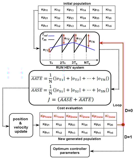
Figure 11.
PSO-based tuning of BEV controllers.
The following steps explain point by point how optimum controllers’ gains are found with the PSO algorithm. When the same steps are almost followed while using the genetic algorithm, only the algorithm philosophy differs:
- Initialize the swarm in a six-dimensional search space.
- For each population particle, run the BEV system for a complete speed profile and evaluate particle’s performance with Equation (38).
- Apply penalty function to exclude unstable PI combinations that resulted in infinite cost values. Infinite or large cost values mean that the actual PMSM speed or torque values are too far from their references.
- Update particles’ speed and position.
- Evaluate the cost of the particle at its new location. If it is smaller than the previous cost value, then update it.
- Keep iterating until the decison signal D (Figure 11) is 1. This last mentioned signal is equal to 1 when the maximum number of iterations is elapsed or the minimum cost is reached.
- Extract the particles that resulted in the smallest cost value.
6. Simulation and Results
To test PSO and GA performance before their integration to the BEV system, the convergence of the two bio inspired algorithms is evaluated with the two benchmark test functions given by Equations (42) and (43) for which the optimum is already known. It is worth noticing that the minimums of F1 and F3 are −18.56 and −0.5231, respectively. Equations (42) and (43) are depicted in Figure 12 and Figure 13, respectively.
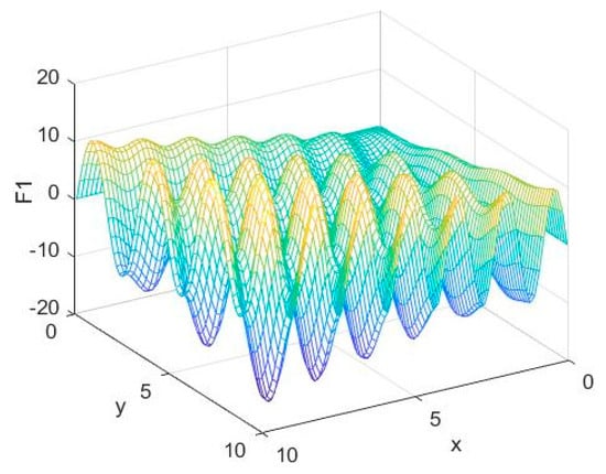
Figure 12.
First-used test function.
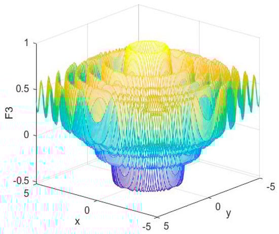
Figure 13.
Second-used test function.
The results of minimizing F1 and F3 with GA and PSO algorithms are depicted in Figure 14 and Figure 15. It could be noticed that both algorithms have converged to the minimum of the employed test functions with a slightly tolerable error, and this confirms the convergence of PSO and GA.
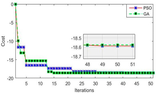
Figure 14.
Cost minimization of F1.
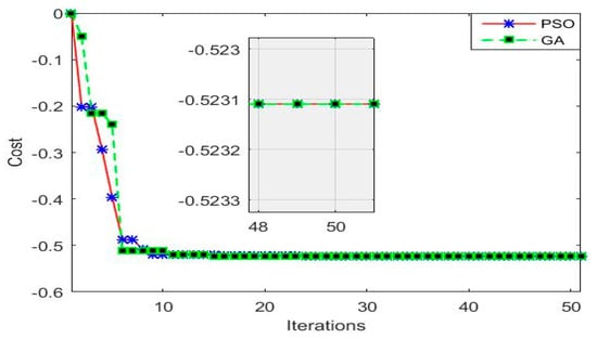
Figure 15.
Cost minimization of F3.
All the simulations carried out through this paper are under a constant wind speed of 10 Kph against vehicle motion and a road slope of 10°. The BEV is subjected to two speed inputs: step-speed input and driving-cycle input speed. For step speed input, we want our response to have minimum overshoot, minimum settling time, and minimum speed and torque steady-state error. For driving-cycle input speed, since the UDDS driving cycle is a series of data points that does not settle, it is meaningless to include peak overshoot or settling time in the design specification. This is why the design specifications for driving-cycle input speed are the minimum instantaneous absolute-torque and speed errors.
6.1. Simple Step Reference input Speed
Figure 16 shows the electric vehicle response when it is subjected to a simple reference speed input of 50 km/h. One can remark form Figure 16 that PSO and GA algorithms yielded a speed response with almost a null peak overshoot, but a trial-an- error approach yielded a relatively faster response with 5% overshoot. From Figure 17, Figure 18, Figure 19, Figure 20, Figure 21 and Figure 22, one can state that the absolute-speed error obtained by either the trial-and-error approach or the intelligent-tuning approach is approximately the same and it is in the order of 10−5 km/h. For absolute torque error, the trial and error approach yielded a mean error of 1.5 N·m, whereas genetic algorithm and particle swarm optimization resulted respectively in an average absolute-torque error of 0.007 N·m and 0.01 N·m.
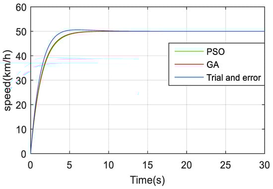
Figure 16.
BEV speed response for simple input speed reference.
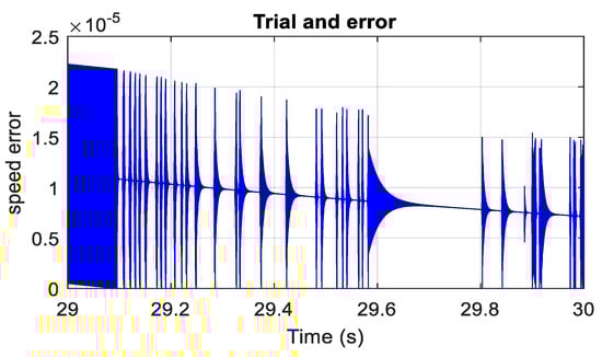
Figure 17.
BEV absolute speed error based on trial and error.
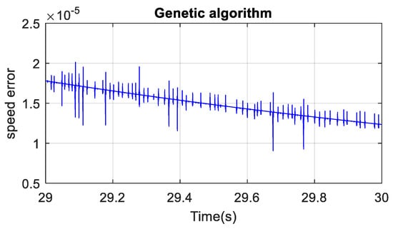
Figure 18.
BEV absolute speed error with GA.
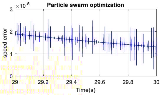
Figure 19.
BEV absolute speed error with PSO.
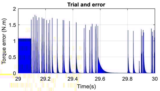
Figure 20.
BEV absolute torque error based on trial and error.
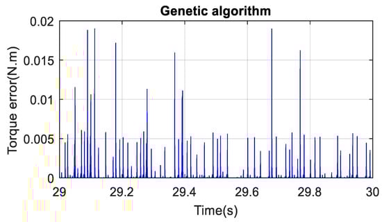
Figure 21.
BEV absolute torque error with GA.
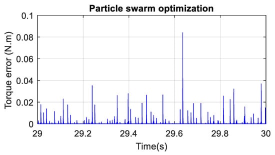
Figure 22.
BEV absolute torque error with PSO.
Figure 23 highlights the cost value for PSO and GA algorithms while minimizing the fitness function J1 given in Equation (37). One can notice the cost value for both algorithms keeps decreasing as the number of iterations increases, which mean that the used-cost function was effectively optimized. From Figure 23, moreover, one can remark that both algorithms converged to the same value, although GA converged faster.
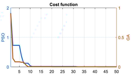
Figure 23.
Cost value for PSO and GA algorithm.
Figure 24 shows the evolution of controller parameters using PSO and GA algorithms. After each iteration, the PID parameters resulting in the minimized cost function given by Equation (37) are kept. Subsequently, the best global cost is deduced with Equations (27) and (28).
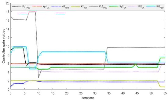
Figure 24.
Best controller position for PSO and GA algorithm.
6.2. Driving Cycle
It is clear enough that in real life an electric vehicle is not subjected to simple-step inputs, but it is subjected to driving cycles with different levels of complexity. City driving cycles are known by their high level of complexity and for their random and abrupt variations that make the control task more difficult. In this section, the electric vehicle was subjected to different international driving cycles, and the friction coefficient is made variable following Equation (7). The electric vehicle control system is now subjected to three international certified driving cycles, and its speed and current loops were tuned to track the reference input driving cycles.
6.2.1. ECE 15 Driving Cycle
Figure 25 shows the BEV speed response and its reference when the ECE15 driving cycle is applied. One can notice that there is almost a perfect match between the actual BEV speed and its reference. This is confirmed by Figure 26, which highlights that the maximum absolute speed error is 3.5 × 10⁻³. From Figure 27, it can be remarked that the BEV torque response precisely follows its reference with a maximum absolute torque error of 0.42 N·m as it is shown in Figure 28.
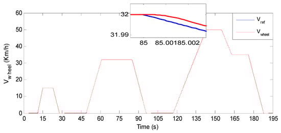
Figure 25.
BEV speed response and its reference for ECE driving cycle.
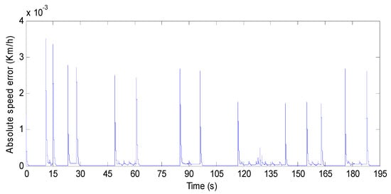
Figure 26.
BEV speed absolute error for ECE driving cycle.
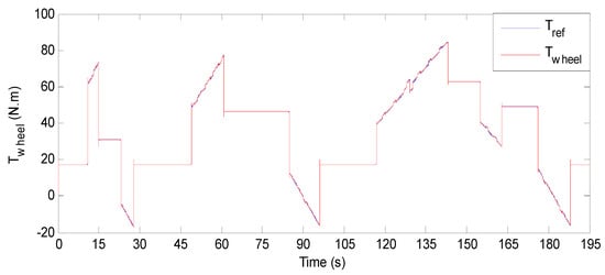
Figure 27.
BEV torque response and its reference for ECE driving cycle.
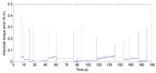
Figure 28.
BEV speed absolute-torque error for ECE driving cycle.
PMSM phase currents are shown in Figure 29; the zooms on that figure show that they are pure sinusoidal and 120 degrees apart, which means that the traction motor operates under balanced or normal conditions. The amplitude of PMSM phase currents depends on BEV torque, and both of them vary in the same manner. When the BEV torque is constant, the phase currents’ amplitude is also constant; when BEV torque increases, the phase currents’ amplitude increases, and when BEV torque decreases, so does the phase current amplitude. One can also conclude from the zooms of Figure 29 that the frequency of PMSM phase currents is variable and depends on vehicle speed. To confirm this, it is necessary to mention that PMSM rotor speed is related to frequency as follows:
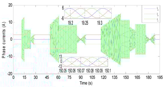
Figure 29.
BEV torque response and its reference for ECE driving cycle.
When t [96 s, 117 s] in Figure 25, the BEV speed or rotor speed is null. According to Equation (43), this means that the f = 0 Hz, which means that the PMSM currents must be constant at that time interval. Indeed, in Figure 29, PMSM phase currents are constant at that time interval, and their sum is null, which means that there is no current flowing to the motor because the vehicle is at rest.
6.2.2. HWFET Driving Cycle
Figure 30 shows the BEV speed response and its reference when HWFET driving cycle is used as input speed reference. The vehicle absolute-speed error is shown in Figure 31 where one can see that the speed error is satisfactory, and it is in the order of 10−3. Figure 32 shows that the BEV torque follows its reference during all of the driving cycle periods. The absolute-torque error is in a narrow band as it is shown in Figure 33 where one can see that the maximum torque error is 0.6 N·m. Figure 34 shows PMSM phase currents during the HWFET driving cycle; their zoom provided in Figure 35 shows a sinusoidal shape with variable amplitude and frequency. From Equation (40), one can conclude that the variable current frequency is due to BEV speed variation. The amplitude of PMSM phase currents depends on BEV torque, and both of them vary in the same manner. When the BEV torque is constant, the phase currents’ amplitude is also constant. When BEV torque increases, the phase currents’ amplitude increases, and when BEV torque decreases, so does the phase current amplitude.
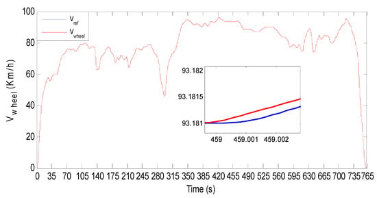
Figure 30.
BEV speed response and its reference for HWEFT driving cycle.
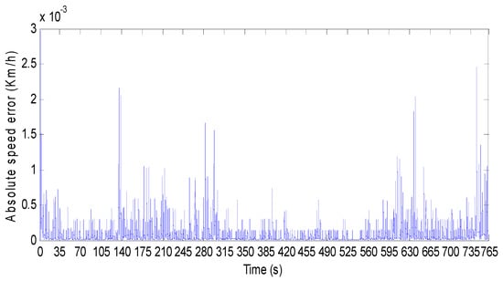
Figure 31.
BEV speed absolute error for HWEFT driving cycle.
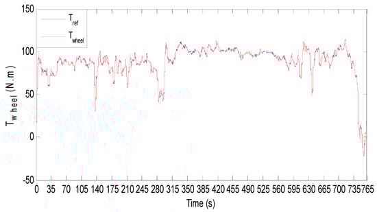
Figure 32.
BEV torque response and its reference for HWEFT driving cycle.
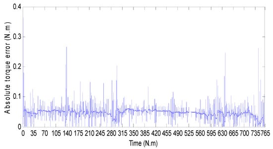
Figure 33.
BEV torque absolute error for HWEFT driving cycle.
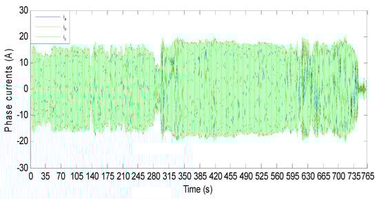
Figure 34.
PMSM phase currents for HWFET driving cycle.
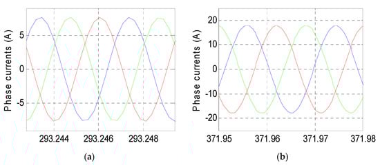
Figure 35.
BEV torque response and its reference for HWEFT driving cycle.
6.3. Robustness against Change of Environmental Parameters
As mentioned in the previous section, the load torque is varying as the vehicle is undergoing a given path. This variation is due to some external and environmental parameters such as road type, which maybe a concrete, snowy, or sandy road. Road slop and wind are also crucial factors that affect the system response. The impact of surface friction on BEV response is shown in Figure 36 where one can see that the BEV response remains always stable with zero steady-state error, which means that the BEV response is robust. Figure 37 shows that the road slope does have an impact on vehicle dynamics, which tend to become slower as the slope angle becomes larger. From Figure 38, it can be concluded that when the speed is negative (which means that the speed is in the same direction as the vehicle), the response becomes faster, and when the speed is against vehicle motion, the vehicle dynamics become slower.
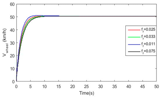
Figure 36.
Effect of variation of surface-friction coefficient on BEV speed response.
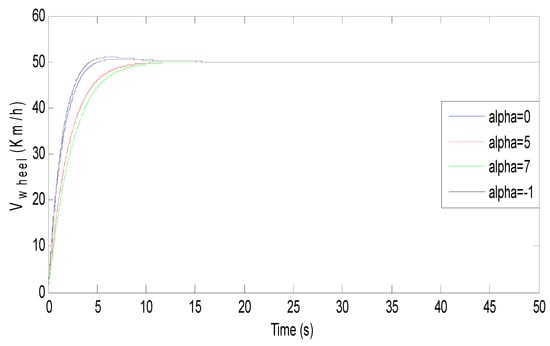
Figure 37.
Effect of variation of surface-friction coefficient on BEV speed response.
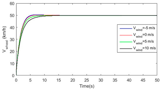
Figure 38.
Wind variation effect of surface-friction coefficient on BEV speed response.
From Figure 39 one can deduce that when wind speed is in the same direction as BEV motion, its response becomes faster and this increases the performance of its speed response in terms of rising and settling time. However, when wind speed is against vehicle motion, the overshoot of the speed response gets lowered and its dynamics becomes relatively slow. Figure 40 confirms that BEV performances gets slow as road slope increases and the inverse is correct. Figure 41 confirms that road type does affect BEV speed response.
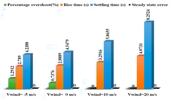
Figure 39.
Wind variation effect on BEV performances.
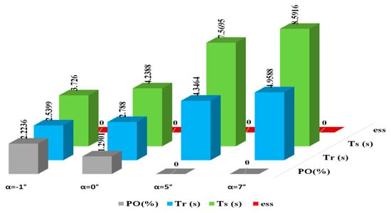
Figure 40.
Road inclination effect on BEV transient performance.
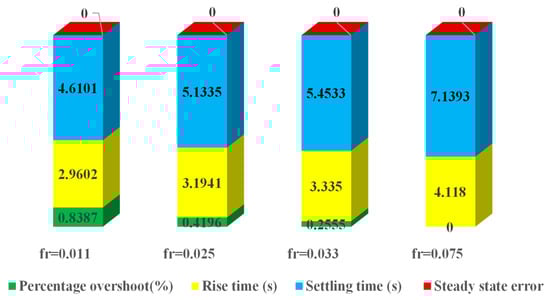
Figure 41.
Wind variation effect on BEV performances.
6.4. Robustness against BEV Parameters Variation
The parameters of any electrical system may be subjected to variations due to different factors such as heat, moisture, and uncertainty of the measurement device. In this section, a robustness analysis is carried out by varying the time constant of some of the EV components, which are the vehicle sensor and inverter. Table 7 shows that the effect of parameter variation is very small. Figure 42 and Figure 43 respectively show the BEV speed response for different inverter and sensor time constants. Changes in inverter and sensor time constants have been made in the interval of −50% to +50% in steps of 25%.
Table 7.
Results of robustness analysis against BEV parameter variation.
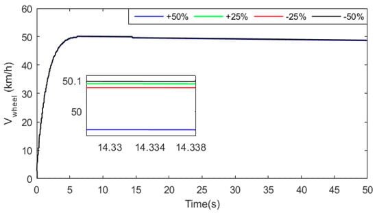
Figure 42.
Effect of inverter time constant variation.
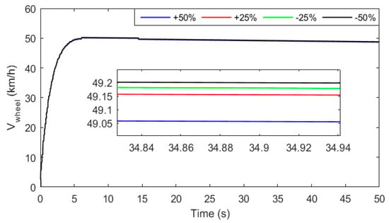
Figure 43.
Effect of sensor time constant variation.
From the zooms of Figure 42 and Figure 43, one can notice that the variation of inverter and sensor time constants do not significantly affect vehicle performace. For instance, a maximum speed deviation of 0.1 km/h was recorded when the varying inverter time remained constant. Moreover, from Figure 43 one can notice that the sensor time constant variation resulted in a maximum speed deviation of 0.2 km/h. These results confirm the effectiveness of intelligent tuning and the robustness of the designed vehicle control system.
7. Conclusions
The speed of the BEV was controlled with the FOC technique, which added a degree of freedom and simplicity to the control by providing decoupling between direct and quadrature axes. PI controllers were used for BEV speed regulations and for PMSM current regulation, which was used to ensure the traction of the electric vehicle. The PI speed and current regulators were tuned with the classical method based on trial and error, and then intelligent tuning was used with PSO and GA algorithms. These two algorithms have succeeded in providing better results, and they have also succeeded in providing a good tradeoff between speed and current control, which was the main problem with the trial-and-error method The electric vehicle was simulated for simple input speed reference and international driving cycles and the simulation results show that the application of the FOC technique along with the efficient tuning of speed and current loops provided satisfactory speed and torque results. Robustness analysis was carried out and the results show that the BEV is robust against the variations of environmental parameters.
Author Contributions
Conceptualization, A.O., N.T. and T.R.; methodology, A.O., N.T., T.R., A.F. and S.N.; software, A.O., N.T. and T.R.; validation, T.R., T.E.A.A., S.S.M.G. and A.F.; formal analysis, A.O., N.T., T.R. and S.N.; investigation, A.O., T.E.A.A. and S.S.M.G.; resources, A.O., T.E.A.A. and S.S.M.G.; data curation, A.O., N.T. and T.R.; writing—original draft preparation, A.O., N.T. and T.R.; writing—review and editing, T.E.A.A., S.S.M.G., A.F. and S.N.; visualization, T.E.A.A., S.S.M.G., A.F. and S.N.; supervision, T.R. and S.S.M.G.; project administration, T.R. and S.S.M.G.; funding acquisition, T.E.A.A., S.S.M.G. and S.N. All authors have read and agreed to the published version of the manuscript.
Funding
This research was supported by Taif University Researchers Supporting Project Number TURSP-2020/34, Taif, Saudi Arabia.
Institutional Review Board Statement
Not applicable.
Informed Consent Statement
Not applicable.
Data Availability Statement
The data presented in this study are available on request from the corresponding author.
Acknowledgments
The authors express their gratitude to Taif University Researchers Supporting Project Number TURSP-2020/34, Taif, Saudi Arabia.
Conflicts of Interest
The authors declare no conflict of interest.
References
- Prakash, P.; Meena, D.C.; Malik, H.; Alotaibi, M.A.; Khan, I.A. A Novel Analytical Approach for Optimal Integration of Renewable Energy Sources in Distribution Systems. Energies 2022, 15, 1341. [Google Scholar] [CrossRef]
- Agrawal, H.; Talwariya, A.; Gill, A.; Singh, A.; Alyami, H.; Alosaimi, W.; Ortega-Mansilla, A. A Fuzzy-Genetic-Based Integration of Renewable Energy Sources and E-Vehicles. Energies 2022, 15, 3300. [Google Scholar] [CrossRef]
- AlKassem, A.; Draou, A.; Alamri, A.; Alharbi, H. Design Analysis of an Optimal Microgrid System for the Integration of Renewable Energy Sources at a University Campus. Sustainability 2022, 14, 4175. [Google Scholar] [CrossRef]
- Sahri, Y.; Belkhier, Y.; Tamalouzt, S.; Ullah, N.; Shaw, R.N.; Chowdhury, M.; Techato, K. Energy Management System for Hybrid PV/Wind/Battery/Fuel Cell in Microgrid-Based Hydrogen and Economical Hybrid Battery/Super Capacitor Energy Storage. Energies 2021, 14, 5722. [Google Scholar] [CrossRef]
- Longo, M.; Yaïci, W.; Zaninelli, D. “Team play” between renewable energy sources and vehicle fleet to decrease air pollution. Sustainability 2015, 8, 27. [Google Scholar] [CrossRef] [Green Version]
- Han, S.; Zhang, B.; Sun, X.; Han, S.; Höök, M. China’s energy transition in the power and transport sectors from a substitution perspective. Energies 2017, 10, 600. [Google Scholar] [CrossRef] [Green Version]
- Sobol, Ł.; Dyjakon, A. The influence of power sources for charging the batteries of electric cars on CO2 emissions during daily driving: A case study from Poland. Energies 2020, 13, 4267. [Google Scholar] [CrossRef]
- Irle, R.; Pontes, J.; Irle, V. Available online: https://www.ev-volumes.com/ (accessed on 16 May 2022).
- Sant, A.V.; Khadkikar, V.; Xiao, W.; Zeineldin, H.H. Four-axis vector-controlled dual-rotor PMSM for plug-in electric vehicles. IEEE Trans. Ind. Electron. 2014, 62, 3202–3212. [Google Scholar] [CrossRef]
- Stippich, A.; Van Der Broeck, C.H.; Sewergin, A.; Wienhausen, A.H.; Neubert, M.; Schülting, P.; Taraborrelli, S.; van Hoek, H.; De Doncker, R.W. Key components of modular propulsion systems for next generation electric vehicles. CPSS Trans. Power Electron. Appl. 2017, 2, 249–258. [Google Scholar] [CrossRef]
- Bai, H. Position Estimation of a PMSM in an Electric Propulsion Ship System Based on High-Frequency Injection. Electronics 2020, 9, 276. [Google Scholar] [CrossRef] [Green Version]
- Khan, M.A.; Zeb, K.; Sathishkumar, P.; Ali, M.U.; Uddin, W.; Hussain, S.; Ishfaq, I.; Cho, H.-G.; Kim, H.J. A novel supercapacitor/lithium-ion hybrid energy system with a fuzzy logic-controlled fast charging and intelligent energy management system. Electronics 2018, 7, 63. [Google Scholar] [CrossRef] [Green Version]
- Suanpang, P.; Pothipassa, P.; Jermsittiparsert, K.; Netwrong, T. Integration of Kouprey-Inspired Optimization Algorithms with Smart Energy Nodes for Sustainable Energy Management of Agricultural Orchards. Energies 2022, 15, 2890. [Google Scholar] [CrossRef]
- Nguyen, T.H.; Nguyen, L.V.; Jung, J.J.; Agbehadji, I.E.; Frimpong, S.O.; Millham, R.C. Bio-inspired approaches for smart energy management: State of the art and challenges. Sustainability 2020, 12, 8495. [Google Scholar] [CrossRef]
- Hasan, U.; Whyte, A.; Al Jassmi, H. A review of the transformation of road transport systems: Are we ready for the next step in artificially intelligent sustainable Transport? Appl. Syst. Innov. 2019, 3, 1. [Google Scholar] [CrossRef] [Green Version]
- Guevara, L.; Auat Cheein, F. The role of 5G technologies: Challenges in smart cities and intelligent transportation systems. Sustainability 2020, 12, 6469. [Google Scholar] [CrossRef]
- Chen, Z.; Cao, Z.; He, X.; Jin, Y.; Li, J.; Chen, P. DoA and DoD estimation and hybrid beamforming for radar-aided mmwave MIMO vehicular communication systems. Electronics 2018, 7, 40. [Google Scholar] [CrossRef] [Green Version]
- Becerra, V.M. Autonomous control of unmanned aerial vehicles. Electronics 2019, 8, 452. [Google Scholar] [CrossRef] [Green Version]
- Wang, W.; Chen, X.; Wang, J. Motor/generator applications in electrified vehicle chassis—A survey. IEEE Trans. Transp. Electrif. 2019, 5, 584–601. [Google Scholar] [CrossRef]
- İnci, M.; Büyük, M.; Demir, M.H.; İlbey, G. A review and research on fuel cell electric vehicles: Topologies, power electronic converters, energy management methods, technical challenges, marketing and future aspects. Renew. Sustain. Energy Rev. 2021, 137, 110648. [Google Scholar] [CrossRef]
- Wang, Z.; Zhou, J.; Rizzoni, G. A review of architectures and control strategies of dual-motor coupling powertrain systems for battery electric vehicles. Renew. Sustain. Energy Rev. 2022, 162, 112455. [Google Scholar] [CrossRef]
- Wang, C.; Xie, Y.; Huang, H.; Liu, P. A review of surrogate safety measures and their applications in connected and automated vehicles safety modeling. Accid. Anal. Prev. 2021, 157, 106157. [Google Scholar] [CrossRef] [PubMed]
- Jiang, B.; Sharma, N.; Liu, Y.; Li, C.; Huang, X. Real-Time FPGA/CPU-Based Simulation of a Full-Electric Vehicle Integrated with a High-Fidelity Electric Drive Model. Energies 2022, 15, 1824. [Google Scholar] [CrossRef]
- Xiao, Z.; Dui-Jia, Z.; Jun-Min, S. A synthesis of methodologies and practices for developing driving cycles. Energy Procedia 2012, 16, 1868–1873. [Google Scholar] [CrossRef] [Green Version]
- Yadav, D.; Verma, A. Performance analysis of permanent magnet synchronous motor drive using particle swarm optimization technique. In Proceedings of the 2016 International Conference on Emerging Trends in Electrical Electronics & Sustainable Energy Systems (ICETEESES), Sultanpur, India, 11–12 March 2016; IEEE: Piscataway, NJ, USA, 2016; pp. 280–285. [Google Scholar]
- Wang, H.; Pei, X.; Yin, B.; Eastham, J.F.; Vagg, C.; Zeng, X. A Novel Double-Sided Offset Stator Axial-Flux Permanent Magnet Motor for Electric Vehicles. World Electr. Veh. J. 2022, 13, 52. [Google Scholar] [CrossRef]
- Sun, X.; Yi, Y.; Zheng, W.; Zhang, T. Robust PI speed tracking control for PMSM system based on convex optimization algorithm. In Proceedings of the 33rd Chinese Control Conference, Nanjing, China, 28–30 July 2014; IEEE: Piscataway, NJ, USA, 2014; pp. 4294–4299. [Google Scholar]
- Liu, K.; Zhu, Z.Q. Quantum genetic algorithm-based parameter estimation of PMSM under variable speed control accounting for system identifiability and VSI nonlinearity. IEEE Trans. Ind. Electron. 2014, 62, 2363–2371. [Google Scholar] [CrossRef]
- Kannan, R.; Gayathri, N.; Natarajan, M.; Sankarkumar, R.S.; Iyer, L.V.; Kar, N.C. Selection of PI controller tuning parameters for speed control of PMSM using biogeography based optimization algorithm. In Proceedings of the 2016 IEEE International Conference on Power Electronics, Drives and Energy Systems (PEDES), Trivandrum, India, 14–17 December 2016; IEEE: Piscataway, NJ, USA, 2016; pp. 1–6. [Google Scholar]
- Qutubuddin, M.D.; Yadaiah, N. Modeling and implementation of brain emotional controller for permanent magnet synchronous motor drive. Eng. Appl. Artif. Intell. 2017, 60, 193–203. [Google Scholar] [CrossRef]
- Baskin, M.; Caglar, B. A modified design of PID controller for permanent magnet synchronous motor drives using particle swarm optimization. In Proceedings of the 2014 16th International Power Electronics and Motion Control Conference and Exposition, Antalya, Turkey, 21–24 September 2014; IEEE: Piscataway, NJ, USA, 2014; pp. 388–393. [Google Scholar]
- Sreejeth, M.; Singh, M.; Kumar, P. Particle swarm optimisation in efficiency improvement of vector controlled surface mounted permanent magnet synchronous motor drive. IET Power Electron. 2015, 8, 760–769. [Google Scholar] [CrossRef]
- Sahri, Y.; Tamalouzt, S.; Hamoudi, F.; Belaid, S.L.; Bajaj, M.; Alharthi, M.M.; Alzaidi, M.S.; Ghoneim, S.S. New intelligent direct power control of DFIG-based wind conversion system by using machine learning under variations of all operating and compensation modes. Energy Rep. 2021, 7, 6394–6412. [Google Scholar] [CrossRef]
- Sayed, K.; Kassem, A.; Saleeb, H.; Alghamdi, A.S.; Abo-Khalil, A.G. Energy-saving of battery electric vehicle powertrain and efficiency improvement during different standard driving cycles. Sustainability 2020, 12, 10466. [Google Scholar] [CrossRef]
- Hussain, S.; Thakur, S.; Shukla, S.; Breslin, J.G.; Jan, Q.; Khan, F.; Ahmad, I.; Marzband, M.; Madden, M.G. A Heuristic Charging Cost Optimization Algorithm for Residential Charging of Electric Vehicles. Energies 2022, 15, 1304. [Google Scholar] [CrossRef]
- Aljohani, T.M.; Ebrahim, A.F.; Mohammed, O. Hybrid microgrid energy management and control based on metaheuristic-driven vector-decoupled algorithm considering intermittent renewable sources and electric vehicles charging lot. Energies 2020, 13, 3423. [Google Scholar] [CrossRef]
- Han, L.; Jiao, X.; Zhang, Z. Recurrent neural network-based adaptive energy management control strategy of plug-in hybrid electric vehicles considering battery aging. Energies 2020, 13, 202. [Google Scholar] [CrossRef] [Green Version]
- Hwang, H.Y.; Chen, J.S. Optimized fuel economy control of power-split hybrid electric vehicle with particle swarm optimization. Energies 2020, 13, 2278. [Google Scholar] [CrossRef]
- Hwang, H.Y.; Lan, T.S.; Chen, J.S. Optimization and application for hydraulic electric hybrid vehicle. Energies 2020, 13, 322. [Google Scholar] [CrossRef] [Green Version]
- He, H.; Liu, D.; Lu, X.; Xu, J. ECO Driving Control for Intelligent Electric Vehicle with Real-Time Energy. Electronics 2021, 10, 2613. [Google Scholar] [CrossRef]
- Kumar, V.; Rana, K.P.S.; Mishra, P. Robust speed control of hybrid electric vehicle using fractional order fuzzy PD and PI controllers in cascade control loop. J. Frankl. Inst. 2016, 353, 1713–1741. [Google Scholar] [CrossRef]
- Zhang, D.; Liu, G.; Zhou, H.; Zhao, W. Adaptive sliding mode fault-tolerant coordination control for four-wheel independently driven electric vehicles. IEEE Trans. Ind. Electron. 2018, 65, 9090–9100. [Google Scholar] [CrossRef]
- Elwer, A.S. A novel technique for tuning PI-controllers in induction motor drive systems for electric vehicle applications. J. Power Electron. 2006, 6, 322–329. [Google Scholar]
- Zhang, D.; Jiang, J. A reliable speed controller for suppressing low frequency concussion of electric vehicle. Microelectron. Reliab. 2018, 88, 1256–1260. [Google Scholar] [CrossRef]
- Huynh, T.A.; Hsieh, M.F. Performance analysis of permanent magnet motors for electric vehicles (EV) traction considering driving cycles. Energies 2018, 11, 1385. [Google Scholar] [CrossRef] [Green Version]
- Ziane, H.; Retif, J.M.; Rekioua, T. Fixed-switching-frequency DTC control for PM synchronous machine with minimum torque ripples. Can. J. Electr. Comput. Eng. 2008, 33, 183–189. [Google Scholar] [CrossRef]
- Metidji, B.; Taib, N.; Baghli, L.; Rekioua, T.; Bacha, S. Low-cost direct torque control algorithm for induction motor without AC phase current sensors. IEEE Trans. Power Electron. 2012, 27, 4132–4139. [Google Scholar] [CrossRef]
Publisher’s Note: MDPI stays neutral with regard to jurisdictional claims in published maps and institutional affiliations. |
© 2022 by the authors. Licensee MDPI, Basel, Switzerland. This article is an open access article distributed under the terms and conditions of the Creative Commons Attribution (CC BY) license (https://creativecommons.org/licenses/by/4.0/).