Analysis of Mobile Robot Control by Reinforcement Learning Algorithm

Abstract

This work presents a Deep Reinforcement Learning algorithm to control a differentially driven mobile robot. This study seeks to explain the influence of different definitions of the environment with a mobile robot on the learning process. In our study, we focus on the Reinforcement Learning algorithm called Deep Deterministic Policy Gradient, which is applicable to continuous action problems. We investigate the effectiveness of different noises, inputs, and cost functions in the neural network learning process. To examine the feature of the presented algorithm, a number of simulations were run, and their results are presented. In the simulations, the mobile robot had to reach a target position in a way that minimizes distance error. Our goal was to optimize the learning process. By analyzing the results, we wanted to recommend a more efficient choice of input and cost functions for future research.

1. Introduction

Machine learning has been strongly developed in recent times [1,2,3]. The advantages of these algorithms enable us to solve important problems in industrial applications, medicine, and many more. The crucial part of machine learning which grows rapidly is deep neural networks. Their application gives the possibility of solving difficult problems in image processing, decision support systems, etc. [1,2,3]. One of the common factors to split the algorithms related with deep neural networks is an approach to learning—supervised and unsupervised. To solve the control problem, which is a subject of this work, the special interest is to take an approach of unsupervised learning, which is Reinforcement Learning (RL) [4]. It enables learning a strategy to solve a problem by teaching an agent using only interactions with the environment.

The basics of Reinforcement Learning are a well-stated part of machine learning. The review of basic algorithms is widely discussed in [4] and survey work [5,6]. An area that has become increasingly important is Deep Reinforcement Learning [2,7,8]. The application of deep neural networks allow to exploit a new field of applications, for instance,  playing games from raw input [7]. In the field of control systems, there are two main types of applications of RL algorithms. The first approach is to extend the control algorithm (such as the PID controller and adaptive controller) by applying the agent to adjust the parameters of the control algorithm [9]. In the second approach, the agent directly controls the object [10,11,12]. The problems of application of the Reinforcement Learning algorithms are described in the work by [13].  Reinforcement Learning has been widely used in robotics [14,15,16]. In our work, we solve the control problem for a mobile robot which has a continuous state space and action space. Therefore, our attention is focused on the actor–critic method. The recent research on the actor–critic method has made great strides towards the development of the Deterministic Policy Gradient (DPG) and its further extension Deep Deterministic Policy Gradient (DDPG) [8,17]. In the work [8], an interesting continuous control algorithm is presented that uses developments such as replay buffer and the target network of the work [7]. It was shown to be capable of learning difficult control algorithms [8,12]. Therefore, in our work, we chose to teach a differentially driven robot.

In this work, we would like to control a two-wheeled mobile robot. In this context, one approach is to apply the classical control algorithms based on explicitly implemented kinematics or dynamics. Classic algorithms are, for instance, vector field-oriented methods [18], transverse functions [19], predictive control [20], etc. Alternatively, the application of Reinforcement Learning is possible to solve this problem [11,21]. The introduction of RL algorithms allow to learn a control policy by interaction with a mobile robot, which is represented as environment. In this approach, dynamics or kinematics do not have to be exploited directly in the design process. It is also possible to learn the control policy by interaction with a robot in experiments [22].

In our work, the main goal is to show a various configurations of the DDPG algorithm applied to control differentially driven mobile robots. The mobile robot is described by kinematics with two alternative input signals. To show the influence on the learning process, we take into account the definition of reward as a variable, the type of control input, and the random exploratory process.

The next part of the paper is organized as follows. Section 2.1 describes the robot model and the definition of the environment for RL. Section 2.2 concentrates on the implementation of the DDPG algorithm. Section 3 shows the learning process with validating tests. This section also points out the main features of the learning process.

2. Problem Definition

In this work, the control problem of a mobile robot is solved by the application of the Reinforcement Learning approach. In general, the target of Reinforcement Learning is to find the optimal policy for the given environment. Learning is carried out based on rewards returned by the environment. The target of the RL algorithm is to find the optimal policy or at least its close approximation. In order to build the environment, firstly, the model of the two-wheeled robot is defined with two sets of inputs consisting of the yaw angular velocity, the forward velocity, and the angular velocities of the right and left wheel. Next, the environment that describes the control problem is proposed. We analyze different rewards to obtain the best final results.

2.1. The Mobile Robot Environment

The kinematics of a differentially driven robot with two wheels has been well studied in the literature [11,18,23,24]. In our work, we consider the following model:

$$\begin{array}{cc}\hfill \dot{q}\left(t\right)& =G\left(q\right(t\left)\right)U\left(t\right)\hfill \\ \hfill U\left(t\right)& =J\mathrm{\Omega }\left(t\right)\hfill \end{array}$$

(1)

where $q\left(t\right)={\left[\begin{array}{ccc}\theta \left(t\right)& x_c\left(t\right)& y_c\left(t\right)\end{array}\right]}^T$ is the state of the robot which consists of the orientation $\theta \left(t\right)$ and the position $x_c\left(t\right)$, $y_c\left(t\right)$. The robot parameters are defined as:

$$\begin{array}{cc}G\left(q\left(t\right)\right)=\left[\begin{array}{cc}1& 0\\ 0& cos\left(\theta \right(t\left)\right)\\ 0& sin\left(\theta \right(t\left)\right)\end{array}\right] & J=\left[\begin{array}{cc}\frac{r}{b}& -\frac{r}{b}\\ \frac{r}{2}& \frac{r}{2}\end{array}\right]\end{array}$$

(2)

where r is the radius of the wheel and b is the tread of the wheel.

In this work, we consider two kinds of input, U and $\mathrm{\Omega }$:

$$\begin{array}{cc}\mathrm{\Omega }\left(t\right)=\left[\begin{array}{c}{\omega }_R\left(t\right)\\ {\omega }_L\left(t\right)\end{array}\right] & U\left(t\right)=\left[\begin{array}{c}\omega \left(t\right)\\ v\left(t\right)\end{array}\right]\end{array}$$

(3)

where ${\omega }_R\left(t\right)$ and ${\omega }_L\left(t\right)$ are the angular velocities of the right and left wheel, $\omega \left(t\right)$ and $v\left(t\right)$ are the yaw angular velocity and the forward velocity of the mobile robot, respectively. The control signals $U\left(t\right)$ and $\mathrm{\Omega }\left(t\right)$ are linked by the invertible matrix J. Therefore, it is possible to calculate $U\left(t\right)$ based on $\mathrm{\Omega }\left(t\right)$ and the other way around. However, in simulations, we show that from the point of view of the Reinforcement Learning algorithms the choice of input will give different results.

The above model is presented in the continuous-time domain, which is typical for the kinematic representation of mobile robots [11,18,23,24]. To implement the model in the environment, it is converted by the Euler forward method to the discrete representation:

$$q_{n+1}=q_n+{\Delta }_{T}G\left(q_n\right)U_n$$

(4)

where $q_n$ denotes $q\left(t_n\right)$ (and similarly for other signals) and ${\Delta }_T$ is the time step.

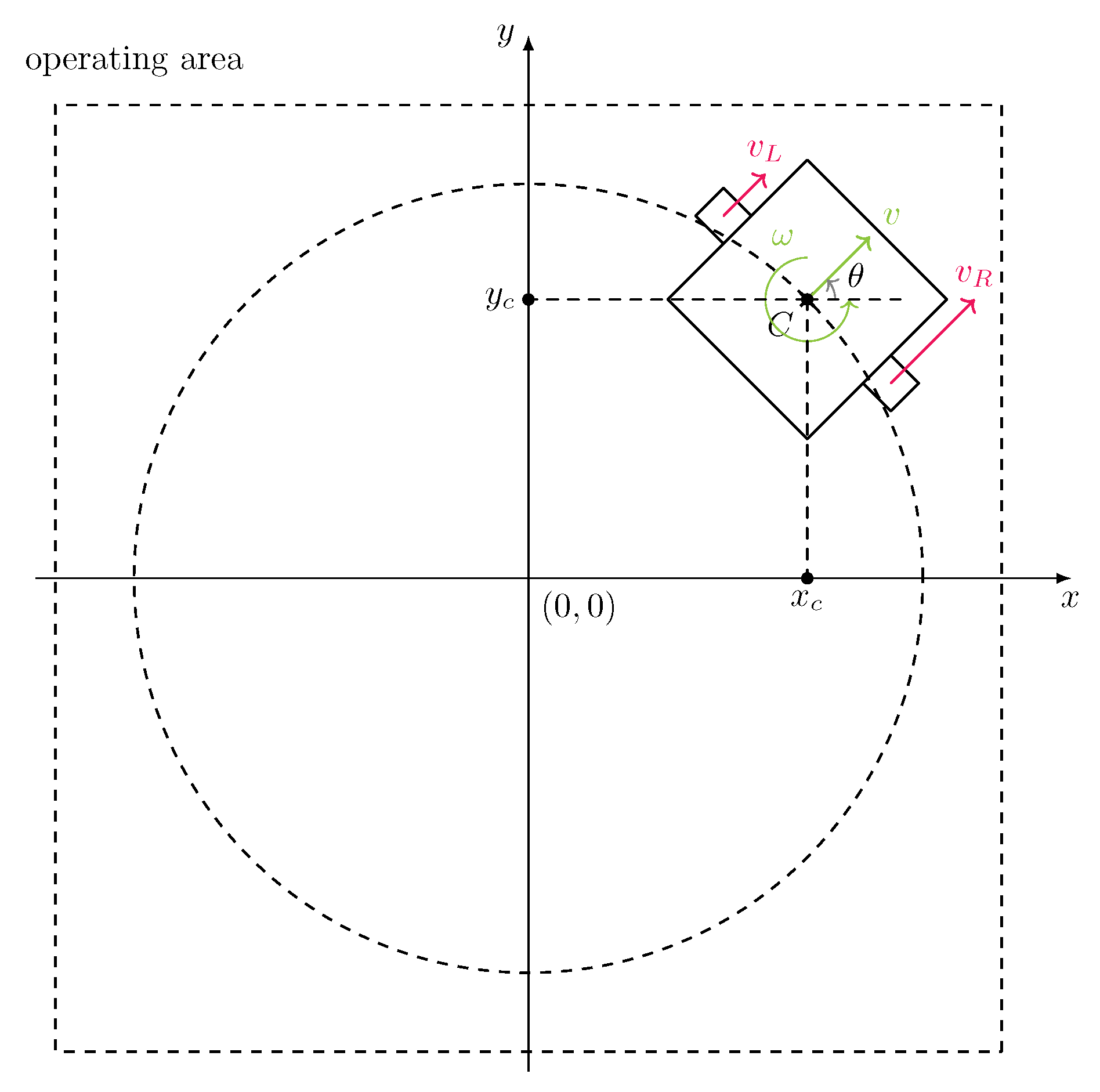
The goal of the work is to drive the robot from the initial state $q_{ini}$ to goal state ${\left[\begin{array}{ccc}0& 0& 0\end{array}\right]}^T$. The initial position of the mobile robot $(x_{ini},y_{ini})$ is randomly chosen in the circle with radius 1 around the point $(0,0)$. The orientation ${\theta }_{ini}$ is also randomly chosen from the range $-\pi$ to $\pi$, so from a practical point of view it does not have limitations. The mobile robot with the state and input variables is presented in Figure 1. The figure also shows possible initial positions. It is worth pointing out that the initial orientation is not constrained, so that the mobile robot can be directed inside or outside the circle.

The crucial part of the Reinforcement Learning approach is the definition of the environment. In our work, the environment is directly incorporated from the discrete model of the mobile robot Equation (4). Therefore, the environment state is $q_n$ and the action is $U_n$ or ${\mathrm{\Omega }}_n$.

To complete the environment, the reward must be designed. We define the auxiliary sets and variables to simplify the description of the reward function. The region in which the robot can move is defined as:

$$Q_{max}=\left\{q:\left|x\right|\le x_{max}\wedge \left|y\right|\le y_{max}\right\}$$

(5)

where $x_{max}$ and $y_{max}$ are the maximum positions around the robot. The orientation is not limited, but it is kept in the range $-\pi$, $\pi$ by $\theta$ signal normalization. The normalization does not influence the possibility of robot rotation, which can be performed without limit.

We also define the distance to $(0,0)$ as:

$$d\left(q\right)=\sqrt{x^2+y^2}$$

(6)

and the norm of orientation:

$$\alpha \left(q\right)=\left|\theta \right|.$$

(7)

The reward is defined in various ways to show its strong influence on the learning process:

$$r_i(q_n,q_{n-1})=-c_i(q_n,q_{n-1})-c_{out}\left(q_n\right)$$

(8)

where $c_i$ is a definition of the cost related to goal achievement and $c_{out}$ is a common term for all costs related to escaping the operating area. The cost $c_{out}$ is given by:

$$c_{out}\left(q_n\right)=\left\{\begin{array}{cc}0,& q_n\in Q_{max}\backslash \partial Q_{max}\hfill \\ 100,& q_n\in \partial Q_{max}\hfill \end{array}\right.$$

(9)

where $\partial Q_{max}$ is a boundary of $Q_{max}$. Furthermore, if $q_n$ reaches the limits of $Q_{max}$ the episode is terminated.

At some cost $c_i$, the additional cost will be added, which partially describes success. It is given by:

$$c_s\left(q_n\right)=\left\{\begin{array}{cc}-100,& q_n\in Q_s\\ 0,& q_n\notin Q_s\end{array}\right.$$

(10)

and is $-100$ (so the reward is 100) inside the region $Q_s$ that is defined around the goal position:

$$Q_s=\left\{q:d\left(q\right)\le d_s\wedge \alpha \left(q\right)\le {\alpha }_s\right\}.$$

(11)

The symbols $d_s$ and ${\alpha }_s$ are the thresholds for distance and orientation. The target of this cost is to promote being close to the goal position.

Now, we propose the set of costs that can be considered to solve the problem of mobile robot control. The general idea of the cost is based on the literature [4,11]; however, it is also fit to the presented problem. Its objective is to drive the robot from initial state to goal state. Some of the cost only takes into account position but some also take the orientation. The first cost is given by

$$c_1\left(q_n\right)=\left|\right|q_n{\left|\right|}^2+c_s\left(q_n\right)$$

(12)

and the goal part is defined similarly to the Lyapunov function. It takes into account the orientation and position with the same weights. The second cost is defined as the weighted part of the distance and the squared orientation:

$$c_2\left(q_n\right)=0.7d\left(q_n\right)+0.3{\theta }^2+c_s\left(q_n\right)$$

(13)

Compared with cost $c_1\left(q_n\right)$, the influence of orientation is decreased. The next cost is the weighted part of absolute orientation and position:

$$c_3\left(q_n\right)=\left|{\theta }_n\right|+200\left(|x_n|+|y_n|\right)+c_s\left(q_n\right)$$

(14)

Its intention is to significantly reduce the absolute position error rather than the orientation. However, in the case of small position error, orientation also becomes important. The following cost function:

$$c_4\left(q_n\right)=\left\{\begin{array}{cc}{x}_n^2+y_n^2-100,& d\left(q_n\right)<d_s\hfill \\ x_n^2+y_n^2,& d\left(q_n\right)\ge d_s\hfill \end{array}\right.$$

(15)

only takes the position into account, and the thresholds only depend on the distance. The next cost is defined as:

$$c_5(q_n,q_{n-1})=\left\{\begin{array}{cc}-100,& d\left(q_n\right)<d_s\hfill \\ 100\left[d\left(q_n\right)-d\left(q_{n-1}\right)\right],& d\left(q_n\right)\ge d_s\hfill \end{array}\right.$$

(16)

and only the position is taken into account. In addition, a decrease in distance error is promoted, which is different from all previous costs. In the region around the goal position, the additional reward is given. A similar approach with incremental reward is given in the work [11]. The following cost:

$$c_6(q_n,q_{n-1})=\left\{\begin{array}{cc}-100,& d\left(q_n\right)<d_s\hfill \\ 1,& d\left(q_n\right)\ge d\left(q_{n-1}\right)\hfill \\ -1,& d\left(q_n\right)<d\left(q_{n-1}\right)\hfill \end{array}\right.$$

(17)

is similar to the previous one (16). However, the increase in distance gives a constant penalty when the decrease in distance gives a reward. The cost with varying weights is defined as

$$\begin{array}{cc}\hfill \gamma \left(q_n\right)& =\left\{\begin{array}{cc}0,& d\left(q_n\right)\le 0\hfill \\ d\left(q_n\right),& 0<d\left(q_n\right)\le 1\hfill \\ 1,& d\left(q_n\right)>0\hfill \end{array}\right.\hfill \\ \hfill c_7\left(q_n\right)& =\gamma \left(q_n\right)d\left(q_n\right)+\left(1-\gamma \left(q_n\right)\right){\theta }_n^2+c_s\left(q_n\right)\hfill \end{array}$$

(18)

to first decrease the position error, then the orientation error. It is also an extension of the cost Equation (13). At the last but not the least cost, we define three thresholds:

$$c_8(q_n,q_{n-1})=\left\{\begin{array}{cc}-50,& d\left(q_n\right)<d_s\wedge \alpha \left(q_n\right)\ge {\alpha }_s\hfill \\ -100,& d\left(q_n\right)<d_s\wedge \alpha \left(q_n\right)<{\alpha }_s\hfill \\ 80\left[d\left(q_n\right)-d\left(q_{n-1}\right)\right]+20\left[\alpha \left(q_n\right)-\alpha \left(q_{n-1}\right)\right],& d\left(q_n\right)\ge d_s\hfill \end{array}\right.$$

(19)

If the distance is above the threshold $d_s$, then the cost is proportional to the decrease in the distance and the orientation error. If the distance is below the threshold then two levels of cost are assigned, respectively, to orientation.

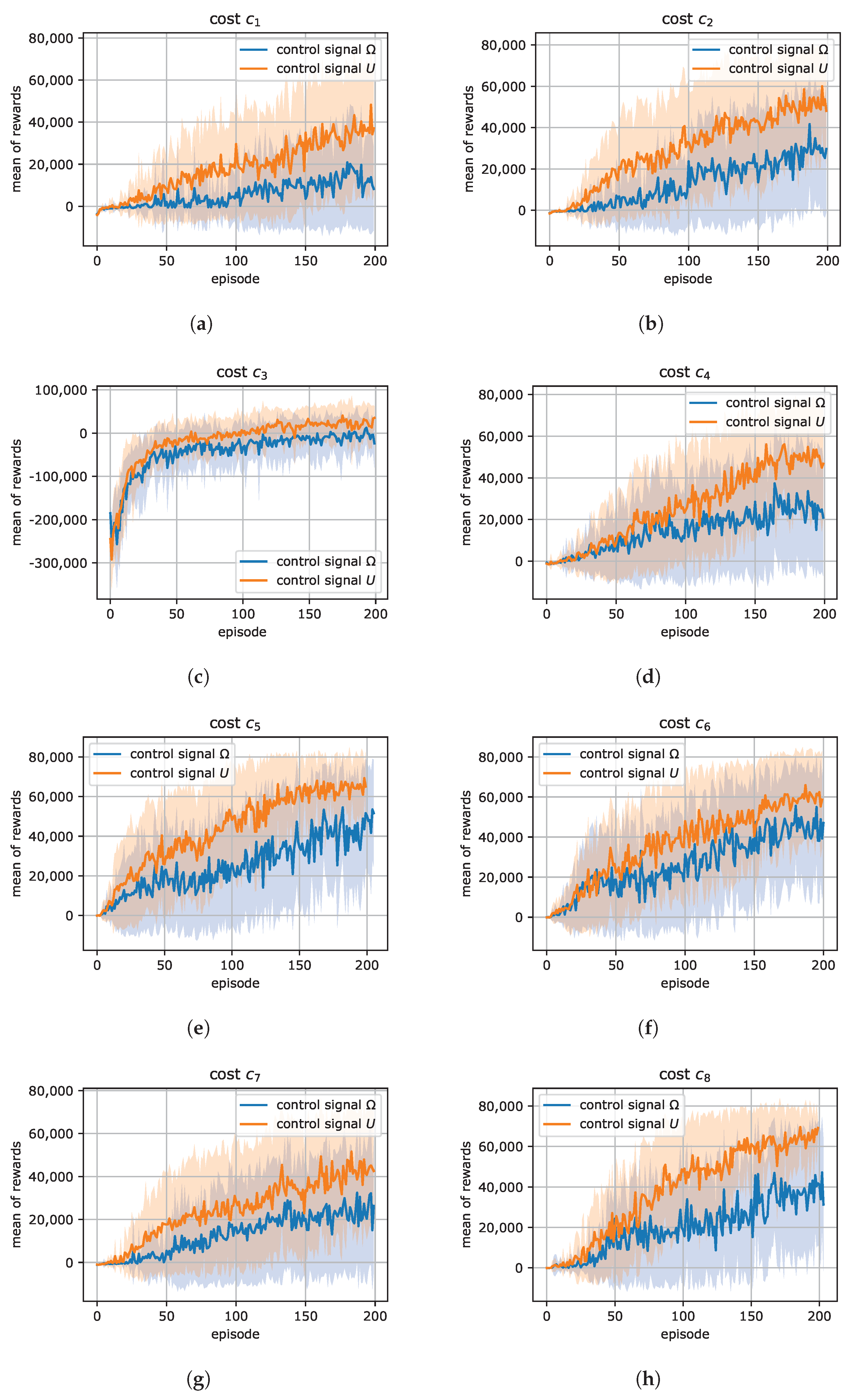
In summary, we defined 8 different costs in which the goal position is taken into account. In

Table 1. Summary of the costs functions.

Cost Type	Attribute
$c_1$	squared norm of the state + additional reward
$c_2$	scaling distance and squared orientation + additional reward
$c_3$	absolute linear function of state + additional reward
$c_4$	only squared distance + additional reward
$c_5$	differential of distance + additional reward
$c_6$	sign of distance differential + additional reward
$c_7$	varying distance and orientation weights during movement + additional reward
$c_8$	scaled differential of distance and orientation + thresholded additional reward

, we present information about attributes for each cost function. The costs $c_1$, $c_2$, $c_3$ and $c_7$, $c_8$ depend on the orientation of the goal, while the costs $c_4$, $c_5$, $c_6$ only take position into account. The costs $c_5$, $c_6$ and $c_8$ depend on the current and the previous state, while others only the current state. Our intention is to check different types of errors and their influence on the learning process and final results.

2.2. The Learning Algorithm

The environment with the mobile robot has continuous input and state. This is one of the crucial aspects of choosing the Reinforcement Learning algorithm. Therefore, we solve the problem by applying the Deep Deterministic Policy Gradient algorithm, which allows to have continuous action space and state space. The DDPG algorithm represents the actor–critic algorithm, which uses approximations by neural networks. The actor decides about the current action based on the policy $\pi \ast \left(a_t\right|s_t)$, which depends on the current state. The critic is described by an action-value function Q. In this work, both the functions Q and $\pi$ are approximated by Deep Neural Network with multiple layers.

In general, the target of Reinforcement Learning and, therefore, the DDPG algorithm, is to find the optimal policy that chooses the action $a_t$ based on the distribution $\pi \ast \left(a_t\right|s_t)$. The learning process is based on the Deterministic Policy Gradient described in the work [8,17]. According to the work [7,8], the important parts of Deep Reinforcement Learning are the replay buffer and target networks.

In our work, the action is a control signal ($\mathrm{\Omega }$ or U) set to mobile robot. We consider two problems where, first, the action is $U_n$ and secondly the action is ${\mathrm{\Omega }}_n$, both defined in Equation (4). The optimal policy $\pi \ast \left(a_t\right|s_t)$ decides the action based on the current state $s_n$. In this work, the environment state $s_n$ is based on the mobile robot model described in the previous section and is equal to $q_n$.

3. Results

This section examines the proposed RL algorithm in the simulations. The parameters of the mobile robot model defined in (1) are based on the literature example [25], and it is called Mini Tracker (MTV3). According to the work [25], we set the wheel radius to $r=26 \mathrm{m}\mathrm{m}$ and platform width to $2b=66 \mathrm{m}\mathrm{m}$, so the model illustrates the actual object. In the beginning of every simulation, the robot is spawned on a circle with a radius $1 \mathrm{m}$ with random orientation. The size of the available robot world is set 5 by 5 $\mathrm{m}$. The goal of the robot is to go to $q=(0,0,0)$ (in some cost functions, orientation is not taken into account). It is also simulated with the time step ${\Delta }_T$ equal to 5 $\mathrm{m}$$\mathrm{s}$.

To approximate the actor and critic described in the Section 2.2, we create 2 types of neural networks, one for the actor (described by $\pi$) and one for the critic (described by Q). Both types have 3 hidden layers, 1 input layer and 1 output layer. In both types, we use the Rectified Linear Unit (ReLU) activation functions for hidden layers. For an actor neural network, we used 16 neurons for each hidden layer and 2 neurons for the output layer with linear activation function. For a critic neural network, we used 32 neurons for each hidden layer and 1 neuron in the output layer with a hyperbolic tangent activation function. Therefore, the control signal is limited. The neural networks are trained by Adam optimizer with mean absolute error (MAE) metrics.

3.1. Simulations

The following section sets out the results of the simulations. The implementation is based on the library keras-rl [26]. We implement two types of robot input described in Equation (3). We prepare eight cost functions described in Equations (12)–(19). To visualize the cost function, the two open-loop movements of the mobile robot are performed, and the rewards for each position are calculated. The trajectories of the robot are shown in Figure 2, and the rewards function is presented in Figure 3. It is worth noticing that left to right has a small orientation error and right to left has a large orientation error. In Figure 3, it is visible that all costs have a different shape. The costs $c_4$, $c_5$, and $c_6$ are the same for both cases because they do not depend on orientation. In costs $c_1$, $c_2$, and $c_7$, the orientation dominates the cost function so much that reverse orientation for movement from right to left is more important than achieving the position $(0,0)$. We also define three vicinity errors parameterized by delta $\delta$ as presented in

Table 2. The vicinity threshold values of distance $d_s$ and orientation ${\alpha }_s$.

$\mathit{\delta }$	${\mathit{d}}_{\mathit{s}}$ ($\mathbf{m}$)	${\mathit{\alpha }}_{\mathit{s}}$ (${}^{\circ }$)
0.8	0.04	24
1.0	0.05	30
1.2	0.06	36

. We check how the DDPG algorithm learns for two starting random types. This noise call is Gaussian White Noise with zero mean and standard deviation 1 and Ornstein Uhlenbeck Process ($\theta =3$, $\sigma =0.5$). Both exploratory noises are linearly annealed to 0 after 800 steps, as is visible in Figure 4, where an example of random process transients are generated. To specify, we describe our single process as a set of different conditions $p_i$ Equation (20), where $i_s$ is an input type, c is a cost type, n is a noise type, and $\delta$ is the accuracy radius. We show that these design aspects can crucially influence the learning process and resulting trajectories. As a result, the number of learning processes and testing simulations is performed to show the influence of the design variables.

$$\begin{array}{cc}\hfill p_i& =\{i_s,c,n,\delta \},where\hfill \\ \hfill i_s& \in I=\{U,\mathrm{\Omega }\}\hfill \\ \hfill c& \in C=\{c_1,c_2,c_3,c_4,c_5,c_6,c_7,c_8\}\hfill \\ \hfill n& \in N=\{GaussianWhiteNoiseProcess,OrnsteinUhlenbeckProcess\}\hfill \\ \hfill \delta & \in D=\{0.8,1.0,1.2\}\hfill \end{array}$$

(20)

With the goal to check the repeatability of the learning process, we run everything 4 times. In summary, it gives 384 learning processes. The hyperparameters of the RL algorithm are defined in

Table 3. The hyperparameters of the learning algorithm.

Parameter Name	Value
forgetting ratio $\gamma$	0.99
target model update	0.001
warm-up steps actor	100
warm-up steps critic	100
number of steps	160,000
maximum episode steps	800
Adam’s learning rate	0.001
Adam’s clip norm	1.0

.

The learned agents are verified in the 10 independent tests, so it gives a total of 3840 data. We have implemented the equations of quality indicators as a tool that helps to determine which tested factor gives better results. These indicators are described as follows:

$$J_{xy}=\frac{1}{N}\sum _{k=0}^N(x_k^2+y_k^2)$$

(21)

$$J_q=\frac{1}{N}\sum _{k=0}^N({\theta }_k^2+x_k^2+y_k^2)$$

(22)

$$J_{qk}=\frac{1}{N}\sum _{k=0}^N({\theta }_k^2+x_k^2+y_k^2)k$$

(23)

$$J_a=\frac{1}{N}\sum _{k=0}^N(v_{1k}^2+{\omega }_{2k}^2)$$

(24)

where N is the number of steps in the validation test. The presented indicators are designed so that a lower value means better results. Because not every cost function includes the orientation of the robot, we choose the performance index $J_{xy}$ to compare every variant in terms of position error. Next, indicator $J_q$ includes the whole state $q=\begin{array}{ccc}[\theta & x& {y]}^T\end{array}$, so we could easily compare the orientation error impact of every solution. We presumed that controllers that include orientation in calculations should have smaller $J_q$ values than the ones that do not include it. The third indicator adds time to our analysis. The lower the value of $J_{qk}$, the quicker our robot minimizes the state errors. Comparing $J_q$ and $J_{qk}$ allows us to define which indicator is better in terms of reaching the final state in finite time. At last, we wanted to compare the energy consumption in every controller. The $J_a$ indicator is calculated based on actions, so the lower values inform us which case is more energy efficient than the others. It is important to mention that the performance index $J_a$ is calculated on v, $\omega$ signals for both types of input to create comparable results.

3.2. Analysis

The analysis in this section is based on the described simulations. We group the data by factors such as control type, cost type, input type, and random process. For the grouped data, the mean value of the performance index is calculated (hence it is denoted as $\overline{J}$). In

Table 4. Comparison of quality indicators depending on the type of control.

Control Type	${\overline{\mathit{J}}}_{\mathit{xy}}$	${\overline{\mathit{J}}}_{\mathit{q}}$	${\overline{\mathit{J}}}_{\mathit{qk}}$	${\overline{\mathit{J}}}_{\mathit{a}}$
$\mathrm{\Omega }$	$3.92\times {10}^{-1}$	$1.84$	$5.77\times {10}^2$	$5.97\times {10}^6$
U	$2.53\times {10}^{-1}$	$1.40$	$4.69\times {10}^2$	$1.93\times {10}^6$

, validation tests are grouped by the control type, which gives two groups of 1920 data. It is relatively easy to see that all types of performance indexes related to error are better for the control type of $\mathrm{\Omega }$.

In

Table 5. Comparison of quality indicators depending on the various cost for control type $\mathrm{\Omega }$.

Cost Type	${\overline{\mathit{J}}}_{\mathit{xy}}$	${\overline{\mathit{J}}}_{\mathit{q}}$	${\overline{\mathit{J}}}_{\mathit{qk}}$	${\overline{\mathit{J}}}_{\mathit{a}}$
$c_1$	$5.77\times {10}^{-1}$	$1.30$	$3.25\times {10}^2$	$6.42\times {10}^6$
$c_2$	$4.23\times {10}^{-1}$	$1.12$	$2.10\times {10}^2$	$4.88\times {10}^6$
$c_3$	$8.52\times {10}^{-2}$	$1.21$	$3.96\times {10}^2$	$5.39\times {10}^6$
$c_4$	$4.03\times {10}^{-1}$	$3.61$	$1.34\times {10}^3$	$6.88\times {10}^6$
$c_5$	$4.39\times {10}^{-1}$	$2.38$	$8.75\times {10}^2$	$6.06\times {10}^6$
$c_6$	$4.36\times {10}^{-1}$	$2.51$	$7.53\times {10}^2$	$5.07\times {10}^6$
$c_7$	$3.10\times {10}^{-1}$	$0.58$	$1.60\times {10}^2$	$7.28\times {10}^6$
$c_8$	$4.59\times {10}^{-1}$	$2.04$	$5.58\times {10}^2$	$5.81\times {10}^6$

and

Table 6. Comparison of quality indicators depending on the various cost for control type U.

Cost Type	${\overline{\mathit{J}}}_{\mathit{xy}}$	${\overline{\mathit{J}}}_{\mathit{q}}$	${\overline{\mathit{J}}}_{\mathit{qk}}$	${\overline{\mathit{J}}}_{\mathit{a}}$
$c_1$	$4.30\times {10}^{-1}$	$6.04\times {10}^{-1}$	$1.78\times {10}^2$	$1.35\times {10}^6$
$c_2$	$2.86\times {10}^{-1}$	$6.68\times {10}^{-1}$	$1.56\times {10}^2$	$2.62\times {10}^6$
$c_3$	$8.19\times {10}^{-2}$	$5.01\times {10}^{-1}$	$1.00\times {10}^2$	$9.53\times {10}^5$
$c_4$	$2.87\times {10}^{-1}$	$3.48$	$1.36\times {10}^3$	$2.96\times {10}^6$
$c_5$	$2.65\times {10}^{-1}$	$2.48$	$9.98\times {10}^2$	$2.03\times {10}^6$
$c_6$	$4.10\times {10}^{-1}$	$2.60$	$8.13\times {10}^2$	$2.15\times {10}^6$
$c_7$	$2.13\times {10}^{-1}$	$6.27\times {10}^{-1}$	$1.27\times {10}^2$	$2.42\times {10}^6$
$c_8$	$4.79\times {10}^{-2}$	$2.41\times {10}^{-1}$	$2.40\times {10}^1$	$9.90\times {10}^5$

, we present data about cost type divided into control types. Analyzing the values in Table 5 and Table 6, we can see that the control type U is better for all indicators. The interesting results have cost type $c_3$ because this cost has a simple formula and good values in Tables. This control type is good where position accuracy is important because the position has a main impact on (14). Analyzing Table 6, we can highlight $c_7$ because of its smallest values in $J_q$ and $J_{qk}$ indicators. This means that we obtain the most accurate final position, but it is worth mentioning that it is also the most energy-consuming type. Even though $c_7$ has the best performance, we should only use it when the robot input is $\mathrm{\Omega }$. When we change our input into U, not only the indicators reach lower values, but also different cost types give better results. Analyzing Table 6, $c_8$ stands out from the others costs because it achieves the lowest values in ${\overline{J}}_{xy}$, ${\overline{J}}_q$, and ${\overline{J}}_{qk}$. Cost type $c_8$ is also better than the others in the ${\overline{J}}_{qk}$ table column, which shows that it has the smallest steady state error. This indicator also says the runtime for this cost type is the smallest. Cost type $c_8$ also has an energy efficient input signal.

Table 7. Comparison of quality indicators depending on the type of random.

Random Type	${\overline{\mathit{J}}}_{\mathit{xy}}$	${\overline{\mathit{J}}}_{\mathit{q}}$	${\overline{\mathit{J}}}_{\mathit{qk}}$	${\overline{\mathit{J}}}_{\mathit{a}}$
Gaussian White Noise	$2.58\times {10}^{-1}$	$1.37$	$4.25\times {10}^2$	$4.72\times {10}^6$
Ornstein Uhlenbeck	$3.86\times {10}^{-1}$	$1.88$	$6.22\times {10}^2$	$3.19\times {10}^6$

shows that Gaussian White Noise gives better configuration results, but the Ornstein Uhlenbeck Process gives lower energy consumption.

The example of robot movement on the X–Y plane is presented in Figure 5 for the single case. It shows one of the best results based on Table 4, Table 5, Table 6 and Table 7. It is visible that for 10 tests and 4 learning tries, the mobile robot moves close to position $(0,0)$. The orientation also has a small error. It is visible that for some starting position, the mobile robot must turn around, which generates a more complicated trajectory. The transient view of the position and orientation is shown in Figure 6 and Figure 7. The waveforms in these figures were calculated as a mean of the absolute value of 10 tests. The transients end up after 200 steps. A little chattering in the orientation transients is also visible. In summary, in the presented example, the transients show that the robot can obtain the goal position for many learning tries and many validation tests.

To examine the learning process, the mean of the rewards obtained was calculated for the data grouped by input signal $\mathrm{\Omega }$ and U and cost type. In Figure 8, it is visible that the learning process for the control signal U obtains better results than for $\mathrm{\Omega }$. It is also worth to point out that reward levels for different costs can be different due to various reward definitions (which was not the case for performance indexes presented in the Tables). Overall, the learning process is difficult due to the nonlinearity of the problem, but the DDPG mostly successfully finds the policy.

4. Conclusions

In summary, we showed that the DDPG learning process is strongly dependent on the reward function. The expression of the goal can be easily described by the cost functions, which do not have to be complicated. Furthermore, an interesting alternative to continuous costs (very similar to the definition of Lyapunov functions) is the application of the thresholds. In the case of a mobile robot, the rewards based on thresholds give good performance indexes. Furthermore, the choice of input signals can be crucial for learning performance, as was visible in the analyzed simulation for U and $\mathrm{\Omega }$. In practice, the presented DDPG algorithm could be used to compensate for the nonlinear part of robot kinematics. The presented example shows mobile robot control for a small area. However, that configuration could be used in trajectory tracking tasks with additional extensions.

References

1. Lecun, Y.; Bengio, Y.; Hinton, G. Deep learning. Nature 2015, 521, 436–444. [Google Scholar] [CrossRef] [PubMed]
2. Arulkumaran, K.; Deisenroth, M.P.; Brundage, M.; Bharath, A.A. Deep Reinforcement Learning: A Brief Survey. IEEE Signal Process. Mag. 2017, 34, 26–38. [Google Scholar] [CrossRef] [Green Version]
3. Schmidhuber, J. Deep Learning in neural networks: An overview. Neural Netw. 2015, 61, 85–117. [Google Scholar] [CrossRef] [Green Version]
4. Sutton, R.S.; Barto, A.G. Reinforcement Learning: An Introduction; MIT Press: Cambridge, MA, USA; London, UK, 2018. [Google Scholar]
5. Kaelbling, L.; Littman, M.; Moore, A. Reinforcement learning: A survey. J. Artif. Intell. Res. 1996, 4, 237–285. [Google Scholar] [CrossRef] [Green Version]
6. Grondman, I.; Busoniu, L.; Lopes, G.A.D.; Babuska, R. A Survey of Actor-Critic Reinforcement Learning: Standard and Natural Policy Gradients. IEEE Trans. Syst. Man Cybern. Part C Appl. Rev. 2012, 42, 1291–1307. [Google Scholar] [CrossRef] [Green Version]
7. Mnih, V.; Kavukcuoglu, K.; Silver, D.; Rusu, A.; Veness, J.; Bellemare, M.; Graves, A.; Riedmiller, M.; Fidjeland, A.; Ostrovski, G.; et al. Human-level control through deep reinforcement learning. Nature 2015, 518, 529–533. [Google Scholar] [CrossRef]
8. Lillicrap, T.; Hunt, J.; Pritzel, A.; Heess, N.; Erez, T.; Tassa, Y.; Silver, D.; Wierstra, D. Continuous control with deep reinforcement learning. arXiv 2015, arXiv:1509.02971. [Google Scholar]
9. Howell, M.; Best, M. On-line PID tuning for engine idle-speed control using continuous action reinforcement learning automata. Control Eng. Pract. 2000, 8, 147–154. [Google Scholar] [CrossRef] [Green Version]
10. Hwangbo, J.; Sa, I.; Siegwart, R.; Hutter, M. Control of a Quadrotor With Reinforcement Learning. IEEE Robot. Autom. Lett. 2017, 2, 2096–2103. [Google Scholar] [CrossRef] [Green Version]
11. Choi, J.; Lee, G.; Lee, C. Reinforcement learning-based dynamic obstacle avoidance and integration of path planning. Intell. Serv. Robot. 2021, 14, 663–677. [Google Scholar] [CrossRef]
12. Bernat, J.; Apanasiewicz, D. Model Free DEAP Controller Learned by Reinforcement Learning DDPG Algorithm. In Proceedings of the 2020 IEEE Biennial Congress of Argentina—IEEE ARGENCON 2020, Resistencia, Argentina, 1–4 December 2020. [Google Scholar]
13. Hafner, R.; Riedmiller, M. Reinforcement learning in feedback control. Mach. Learn. 2011, 84, 137–169. [Google Scholar] [CrossRef] [Green Version]
14. Kober, J.; Bagnell, J.A.; Peters, J. Reinforcement learning in robotics: A survey. Int. J. Robot. Res. 2013, 32, 1238–1274. [Google Scholar] [CrossRef] [Green Version]
15. Muzio, A.; Maximo, M.; Yoneyama, T. Deep Reinforcement Learning for Humanoid Robot Behaviors. J. Intell. Robot. Syst. Theory Appl. 2022, 105, 1–6. [Google Scholar] [CrossRef]
16. Muratore, F.; Ramos, F.; Turk, G.; Yu, W.; Gienger, M.; Peters, J. Robot Learning From Randomized Simulations: A Review. Front. Robot. AI 2022, 9, 799893. [Google Scholar] [CrossRef] [PubMed]
17. Silver, D.; Lever, G.; Heess, N.; Degris, T.; Wierstra, D.; Riedmiller, M. Deterministic policy gradient algorithms. In Proceedings of the International Conference on Machine Learning, Bejing, China, 22–24 June 2014; Volume 1, pp. 605–619. [Google Scholar]
18. Michałek, M.; Kozłowski, K. Vector-field-orientation feedback control method for a differentially driven vehicle. IEEE Trans. Control Syst. Technol. 2010, 18, 45–65. [Google Scholar] [CrossRef]
19. Pazderski, D. Waypoint Following for Differentially Driven Wheeled Robots with Limited Velocity Perturbations: Asymptotic and Practical Stabilization Using Transverse Function Approach. J. Intell. Robot. Syst. Theory Appl. 2017, 85, 553–575. [Google Scholar] [CrossRef] [Green Version]
20. Nascimento, T.; Dórea, C.; Gonçalves, L. Nonholonomic mobile robots’ trajectory tracking model predictive control: A survey. Robotica 2018, 36, 676–696. [Google Scholar] [CrossRef]
21. Tai, L.; Paolo, G.; Liu, M. Virtual-to-real Deep Reinforcement Learning: Continuous Control of Mobile Robots for Mapless Navigation. CoRR 2017. Available online: http://xxx.lanl.gov/abs/1703.00420 (accessed on 1 April 2022).
22. Levine, S.; Finn, C.; Darrell, T.; Abbeel, P. End-to-End Training of Deep Visuomotor Policies. J. Mach. Learn. Res. 2016, 17, 1334–1373. [Google Scholar]
23. Kolmanovsky, I.; McClamroch, N. Developments in nonholonomic control problems. IEEE Control Syst. Mag. 1995, 15, 20–36. [Google Scholar] [CrossRef]
24. M’Closkey, R.; Murray, R. Exponential stabilization of driftless nonlinear control systems using homogeneous feedback. IEEE Trans. Autom. Control 1997, 42, 614–628. [Google Scholar] [CrossRef]
25. Dariusz, P.; Maciej, M. Sterowanie Robotów Mobilnych. Laboratorium, 1st ed.; Wydawnictwo Politechniki Poznańskiej/Poznan University of Technology: Poznan Poland, 2012. [Google Scholar]
26. Plappert, M. keras-rl. 2016. Available online: https://github.com/keras-rl/keras-rl (accessed on 1 April 2022).
Figure 1. The mobile robot with the input and state variables.
Electronics 11 01754 g001
Figure 2. The two example movements of a mobile robot in visual reward functions: left to right (a) and right to left (b).
Electronics 11 01754 g002
Figure 3. All rewards ( c 1 c 8 ), respectively (ah), presented, for example, movement of the mobile robot.
Electronics 11 01754 g003
Figure 4. The example of noise added to action to provide exploration: Gaussian White Noise Process (a) and Ornstein Uhlenbeck Process (b).
Electronics 11 01754 g004
Figure 5. Example result for U control type, c 8 cost type, Gaussian White Noise Process and δ = 0.8 on X-Y plane.
Electronics 11 01754 g005
Figure 6. Error x and y for example result for U control type, c 8 cost type, Gaussian White Noise Process and δ = 0.8 .
Electronics 11 01754 g006
Figure 7. Error θ for example result for U control type, c 8 cost type, Gaussian White Noise Process, and δ = 0.8 .
Electronics 11 01754 g007
Figure 8. The mean of rewards in the episode for control signals (Ω and U) and all cost types (ah).
Electronics 11 01754 g008