Article

An Improved Multi-Objective Deep Reinforcement Learning Algorithm Based on Envelope Update

1
School of Microelectronics and Control Engineering, Changzhou University, Changzhou 213164, China
2
School of Computer Science and Artificial Intelligence, Changzhou University, Changzhou 213164, China
*
Author to whom correspondence should be addressed.
Electronics 2022, 11(16), 2479; https://doi.org/10.3390/electronics11162479
Submission received: 12 July 2022 / Revised: 30 July 2022 / Accepted: 5 August 2022 / Published: 9 August 2022

Abstract

:
Multi-objective reinforcement learning (MORL) aims to uniformly approximate the Pareto frontier in multi-objective decision-making problems, which suffers from insufficient exploration and unstable convergence. We propose a multi-objective deep reinforcement learning algorithm (envelope with dueling structure, Noisynet, and soft update (EDNs)) to improve the ability of the agent to learn optimal multi-objective strategies. Firstly, the EDNs algorithm uses neural networks to approximate the value function and update the parameters based on the convex envelope of the solution boundary. Then, the DQN structure is replaced with the dueling structure, and the state value function is split into the dominance function and value function to make it converge faster. Secondly, the Noisynet method is used to add exploration noise to the neural network parameters to make the agent have a more efficient exploration ability. Finally, the soft update method updates the target network parameters to stabilize the training procedure. We use the DST environment as a case study, and the experimental results show that the EDNs algorithm has better stability and exploration capability than the EMODRL algorithm. In 1000 episodes, the EDNs algorithm improved the coverage by 5.39% and reduced the adaptation error by 36.87%.

1. Introduction

In recent years, as research into reinforcement learning (RL) has continued, researchers have proposed models that are applicable to a variety of tasks. For single-objective tasks, the agent usually knows the task preferences in advance. The developer makes a fixed choice to maximize future rewards by selecting the optimal decision in the form of a scalar reward [1,2,3,4]. However, in reality, tasks are usually in the form of multiple objectives, each with different priorities, which may conflict with each other. The priority of one of the goals may hinder the success of the other, so the applicability of the strategies learned through single goals is limited in scenarios with different preferences. Multi-objective reinforcement learning (MORL) [5,6] integrates RL and multi-objective optimization by replacing scalar rewards with reward vectors in single-objective tasks, aiming at solving sequential decision problems of the agent in complex environments.
MORL is mainly divided into the categories of single-strategy algorithms and multi-strategy algorithms. Single-strategy MORL [7,8] uses a linearly weighted scalarization method to decompose multiple objectives into a single objective for processing. However, due to the dimensionality reduction of the objective space, single-strategy MORL can only learn the optimal policy with a single weight preference. Multi-strategy MORL learns generalized expectation value functions in objective preferences [9]. Unlike learning each preference value function independently, multi-strategy MORL can learn multiple policies in a single run.
Current multi-strategy MORL methods effectively combine preference values to derive an expectation value function for decision-making or learning. This linear approach identifies the expected payoff strategies for the convex covering set (ccs), where the ccs is a subset of the Pareto covering set [10]. However, in practice, problems such as insufficient exploration and unstable convergence of the agent often lead to difficulties in learning optimal preferences and finding balanced multi-objective solutions [11].
Considering the shortcomings of the existing multi-strategy MORL algorithm, this paper improves the standard DQN algorithm framework and proposes a novel MODRL algorithm (envelope with dueling structure, Noisynet, and soft update, EDNs).
The specific contributions of this paper are as follows:
  • Replacing the traditional DQN structure with a dueling structure. Splitting the state value function into the advantage and value functions to avoid unnecessary value evaluation and make the model converge faster.
  • Adding exploration noise to the neural network parameters using the Noisynet method, which bring persistent, complex, state-independent random perturbations to the strategy and make the agent efficient in exploration.
  • Replacing the traditional DQN parameter update with a soft parameter update to ensure that the target network is updated at each iteration. Improving the training speed and stabilizing the training procedure.
  • A hindsight experience replay approach [12] is used to update the utility-based multi-objective Q-network with a strategy that allows the algorithm to learn more efficiently by reusing different sampling preferences.
The rest of the paper is structured as follows. Section 2 recalls the necessary background of multi-objective optimization, the classical DQN algorithms, multi-objective deep reinforcement learning (MODRL), and envelope update methods. In Section 3, we improve the network structure based on envelope updating, adding exploration noise to the network parameters and replacing the DQN update method with soft updates. In Section 4, we conduct experiments in the Deep Sea Treasure (DST) environment, where DST is the environment used to verify the performance of the MORL algorithm. The experimental results show that the algorithm has better stability and exploration capability compared to other algorithms being compared and improves the efficiency of the agent in learning multi-objective policies. Section 5 describes work related to the multi-strategy MORL algorithm. Section 6 reviews our work and describes future work.

2. Related Work

MORL is a subfield of RL that finds optimal solutions for two or more objectives. We refer to this solution process as multi-objective optimization (MOO). In recent years, many studies have transformed MOO into single-objective optimization (SOO) problems by scalarizing functions, the class of methods of which is called single-strategy MORL. The multiobjective fractional programming problem was studied by Dubey et al. [13,14]. Vamplew et al. [15] proposed to scalarize functions in a simple linear weighting way to achieve the transformation of MOO. Van et al. [16] proposed a Chebyshev scalarization method based on the study of Vamplew, which solved the problem that the learned strategy could not converge at the Pareto concave boundary. Dazeley et al. [17] proposed a single-strategy MORL with softmax as an action-oriented approach by combining the Q-learning algorithm. Overall, due to the dimensionality reduction of the target space, the single-strategy MORL can only learn the optimal policy with a single weight preference.
Multi-strategy MORL can learn multiple strategies in a single run. Abels et al. [18] proposed a method based on generalized vector Q-functions, approximated by weighted conditional networks (CNs), using diverse experience replay for sample-efficient learning to avoid catastrophic forgetting in dynamic preference settings. Xu et al. [19] addressed the continuity problem and proposed a new prediction model to find the set of Pareto solutions. They constructed a set of continuous Pareto-optimal solutions by Pareto analysis and interpolation. Thiago et al. [20] differed from the others by proposing a hybrid MOO approach that can accelerate convergence to similar strategies by prior knowledge from past iterations. In addition to the studies above, improvements to the MORL framework have also been studied. Tajmajer et al. [21] proposed a modular DQN algorithm, where the first three DQN networks work in parallel, and each DQN performs a different optimization task. Then, the framework introduces decision values and weight vectors for each DQN for the selection of actions by the agent, where the decision values are related to the optimization goals of the DQN networks. Finally, the output of each DQN is weighted under specific weight preferences using a scalarization method to obtain the final output. Thanh et al. [22] proposed a more advanced modular multi-objective deep learning framework based on Tajmajer’s research, which separates the neural network structure, the deep reinforcement learning algorithm, and the task environment. The network configuration module sets the number of layers, size, input, and output of the neural network, and the policy network generates the corresponding network structure based on the configuration information. Then, the deep reinforcement learning algorithm performs the training task based on the configured neural network and the environment information. In this framework, only different environments and agents must be provided to train different tasks. Nguyen et al. [23] introduced the asynchronous actor–critic framework to adjust the agent behavior by weighting and scalarizing different objective functions to achieve the specified goals effectively.
Multi-strategy MORL can combine the preferences with the expectations in a linear manner to derive the learned expectation function. However, in the current study, some researchers have only proposed simple modular MORL frameworks that weight the output under specific weight preferences to obtain the final output. The researchers did not consider the improvement of the network structure of MORL. The traditional MORL network structure will have disadvantages such as slow convergence speed and poor stability, while the dueling network structure splits the state value function into an advantage function and value function to avoid unnecessary value evaluation and improve the convergence speed and stability. Some other researchers simply optimized the action selection, ignoring the lack of exploration ability. Adding noise to the parameters of the neural network using the Noisynet method can bring persistent, complex, and state-independent random perturbations to the strategy, making the agent have efficient exploration capability. In addition, current research continues to use the traditional network update approach, which also results in slower convergence of the agent, while soft update ensures that the target network is updated at each iteration, allowing for faster training of the algorithm. In general, the current research suffers from insufficient exploration ability and unstable convergence, which will lead to difficulties in learning the optimal preferences and finding the optimal multi-objective solution.

3. Background

3.1. Multi-Objective Optimization

Multi-objective optimization tasks require two or more objectives to be accomplished simultaneously. However, different optimization objectives often conflict with each other. Optimizing one of the objectives alone may result in a loss of performance of the other objectives, which is not easy to have a unique optimal solution in a multi-objective optimization task [24]. The multi-objective optimization problem is defined as shown in Equation (1).
f ( X ) = f 1 ( X ) , f 2 ( X ) , , f m ( X ) s . t . g l ( X ) 0 l = 1 , 2 , , L
where f i ( X ) represents the ith objective function, g l ( X ) represents the lth constraint function, m represents the number of objective functions (the m optimization objectives conflict with each other), and L represents the number of constraint functions. The goal of multi-objective optimization is to find a set of optimal solutions X * = x 1 * , x 2 * , , x n * , to make f X * reach the optimum while satisfying all constraints, and the Pareto dominance relation is usually used to construct the Pareto-optimal solution [25].
For different optimization objectives f i ( X ) , the optimal condition may be to maximize the objective function or to minimize the objective function. We considered that the objective of RL is to maximize the expected payoff of the agent, so all objective functions are uniformly transformed into maximization objective functions; the expression is Equation (2).
min f i ( X ) = max f i ( X )

3.2. DQN

The Q-learning [26] algorithm uses Q tables to record Q values for each action in each state and update them iteratively, which is suitable for relatively small-scale problems. However, in practice, the state space may be huge or even continuous, which makes it impossible to use the table to save, so the value function can be used to approximate it. Value functions such as neural networks called Q-networks can be linear or nonlinear. In recent years, introducing deep learning structures such as convolutional neural networks and recurrent neural networks in RL has become a trend. DQN takes r + γ max a Q s , a ; θ as the target Q value and defines the loss function based on the deviation between the network output Q value and the target Q value, as shown in Equation (3).
L ( w ) = E r + γ max a Q s , a ; θ Q ( s , a ; θ ) 2
where s , a represents the next status and action after the status s takes action a and Q ( s , a ; θ ) represents the output value of the Q-network. In the calculation, the weight of the deep Q-network can be updated by random gradient descent.

3.3. Multi-Objective Deep Reinforcement Learning

MODRL integrates deep learning with MORL to solve multi-objective optimization problems with higher spatial dimensionality.
The classical MODRL network structure is displayed in Figure 1, and the input and fully connected layers of the network are consistent with traditional deep reinforcement learning. Because MODRL needs to consider multiple optimization objectives simultaneously, there are n groups of nodes at the output end of the network, where n represents the number of optimization objectives, each group of nodes has m child nodes, and the number of child nodes is equal to the size of the behavior space. In addition, the output of the network provides a weight vector according to the relative importance of different optimization objectives. The final output is obtained according to the combination of the output and weights of each group of nodes.

3.4. Envelope Update Method

Single-strategy MODRL runs each single-objective deep reinforcement learning algorithm independently based on a given preference vector, guided by scalarized rewards. However, single-strategy MODRL can only find one Pareto-optimal solution at a time, so it is often necessary to set up multiple sets of preference vectors to train the algorithm multiple times on multi-objective problems. However, this approach will result in the scalarized MODRL algorithm not being able to approach the Pareto boundary uniformly, and the performance is poor in practical applications.
The EMODRL algorithm [27] uses an envelope approach to update the value function and network parameters, i.e., the value function is updated based on the vector form. The neural network parameters are updated using a convex envelope of the solution boundary. The envelope update approach extends the Bellman equations of the Q-learning algorithm in single-objective RL to a multi-objective scenario with the Bellman equations for Q-learning, as shown in Equation (4).
( T Q ) ( s , a ) = R s s , a + γ E s ( H Q ) s , γ < 1
where T is the Bellman optimal operator, R s s , a is the immediate reward in scalar form obtained by the agent after performing action a in state s and transiting to the state s , γ is the discount factor, and H is the optimal operator for the value of the behavior under state s . The H operator is defined as in Equation (5).
( H Q ) s = sup a A Q s , a
The envelope update method extends the Bellman optimal operator T under a single objective to a multi-objective Bellman optimal operator T . This method extends immediate rewards and behavioral values in the scalar form to vector form. The method provides a preference vector ω of length m ( m > 2 ) , and m represents the number of optimization objectives. Therefore, the envelope update method is based on updating the behavioral value function in vector form, and the Bellman equation under multiple objectives is shown in Equation (6).
( T Q ) ( s , a , ω ) = R s s , a + γ E s ( H Q ) s , ω , γ < 1
where H is the optimal operator for the behavioral value vector corresponding to state s in the multi-objective scenario; the expression is Equation (7).
( H Q ) ( s , ω ) = arg Q sup a A , ω Ω ω T Q s , a , ω
where ω is the preference vector passed into the network along with state s and behavior a. ω is the preference vector used to scalarize the behavior value vector Q s , a , ω output from the network.
Given a scalar preference vector ω , an upper bound is found by adjusting the preference vector ω and behavior a of the network input. Finally, an optimal multi-objective behavior value vector Q s , a , ω is returned according to the upper bound corresponding to a , ω . In short, H solves the convex envelope of the current solution boundary to optimize the multi-objective behavioral value, not only on the behavior space, but also by adjusting ω to optimize the multi-objective behavioral value function given the preference vector ω .

4. EDNs Algorithm

4.1. Dueling Network

The traditional DQN algorithm uses a neural network to approximate the behavior value function. The algorithm inputs states as observations to the network, outputs the value corresponding to each action in the current state, then estimates each value. However, in many states, the agent does not need to change the action to adapt to the new state. Therefore, evaluating the value of such state–action pairs is not efficient.
The dueling network structure [28,29] considers that each behavior can bring different advantages and avoid unnecessary action evaluation. The Q value can be estimated more accurately and has a faster convergence speed, which is done by introducing two branching networks after the fully connected layer. One network is used to predict the state value; the other is used to predict the advantage of each action. Finally, the results of these two branches are combined to output the behavior value.
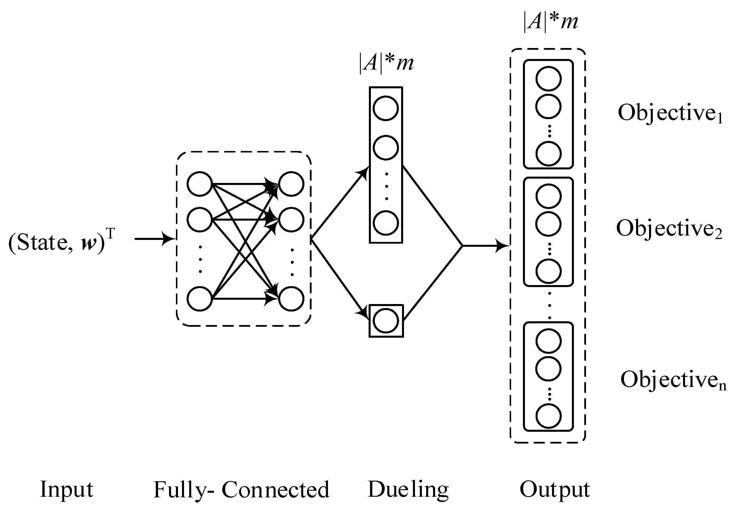
The MODRL algorithm also uses a deep neural network to approximate the behavioral value function. This update of the behavioral value function using the envelope update method requires the state of the agent as an input to the network and the preference vector used for scalarization as a conditional input to the network. Unlike the critic network structure proposed by Treesatayapun et al. [30], as shown in Figure 2, dueling MODRL introduces a dueling structure based on the MODRL network framework. The network framework includes two fully connected layers. The output layer includes n groups of nodes with | A | elements in each group, where m represents the number of optimization targets and | A | represents the size of the behavior space, and all neurons are activated using Relu. The network output is a vector of n sets of behavioral values of size | A | , which makes behavior selection very difficult. However, introducing the dueling network into the network framework of MODRL can make behavior selection easier by fully considering the advantages of each behavior.

4.2. Exploring Noise

Exploration and exploitation are crucial in RL algorithms, determining whether the agent can obtain an optimal solution. If the agent chooses the action with the maximum behavioral value to execute each time, the strategy will converge faster. However, due to the low level of exploration of the environment, many state transitions are not sampled. The corresponding behavioral values are not updated, resulting in a converged strategy that is not optimal. Therefore, the agent should try to explore the unknown regions of the environment during the learning process so that the final strategy is as globally optimal as possible [31].
In the standard DQN algorithm, the agent usually uses the ε -greedy strategy to balance exploration and exploitation. We generally set ε ( 0 < ε 1 ) to a large value at the beginning of the training algorithm, then ε gradually decreases it as the number of training sessions increases. However, there is significant uncertainty in the initialization of ε when using the ε -greedy strategy in RL algorithms. When the initialized ε is small, the probability of an agent reaching a certain state will be low. The agent is unable to perform global exploration, which can lead to a learned strategy that is not optimal. In complex environments, even a larger initial value of ε will lead to insufficient exploration, because the agent will be limited by the termination conditions and the number of episodes. In simpler environments, larger initial values may lead to unnecessary exploration by the agent, resulting in a decrease in the convergence rate. Therefore, an unreasonable setting of the initial value of ε may significantly affect the learning outcome of the agent [32].
In order to improve the efficiency of exploring the agent in multi-objective optimization scenarios, this paper uses the the Noisynet method to add random perturbations to the parameters of the neural network to bring persistent, complex, and state-independent perturbations to the agent strategies. We added parametric noise to the neurons of the fully connected layer of the dueling MODRL network and to automatically adjust the intensity of the noise during the training of the algorithm, so that the output of the network has a certain degree of randomness.
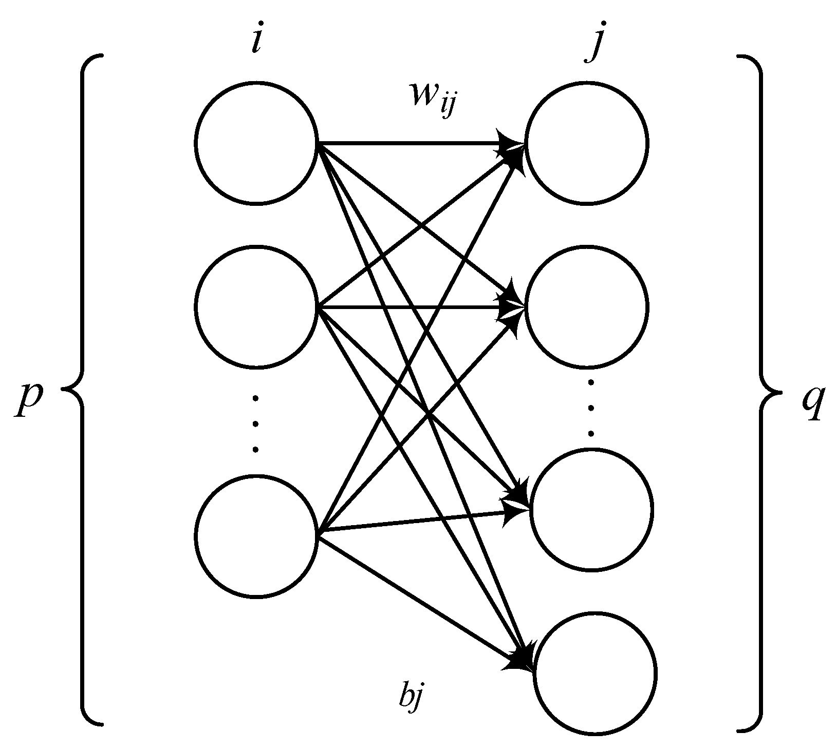
For a linear fully connected layer with p inputs and q outputs, the model is presented in Figure 3. The mathematical representation is y = w x + b , where w is the weight and b is the bias term, w R q × p , x R p , b R q . If random noise is added to the parameters w and b of the fully connected layer, then w μ w + σ w ε w , b μ b + σ b ε b , where ε is the random noise parameter and ⊙ represents elementwise multiplication [33]. The mathematical representation of a fully connected linear layer with noise is displayed in Equation (8).
y = μ w + σ w ε w x + μ b + σ b ε b
The parameters μ w , σ w , and μ b are variable, and the parameters are constant ε w , ε b . Since the DQN and its improved algorithms are generally single-threaded and use decomposed Gaussian noise in order to reduce the computation time, only p + q random noises are needed. For each neuron, the noise of w i j is ε i , j w = f ε i f ε j and the noise of b j is ε j b = f ε j , where f ( x ) = sgn ( x ) | x | .

4.3. Soft Update of the Target Network

The traditional DQN introduces the target network based on the behavioral network in order to enhance the stability of the algorithm. The behavioral network clones its parameters to the target network after updating a certain number of steps, so that the parameter updates remain relatively stable in the updates within a certain number of steps. The update frequency of the target network is adjusted by modifying the update interval of the target network. The larger the update interval of the target network, the more stable the algorithm is, but the convergence speed is relatively slow.
The soft update ensures that the target network is updated at each iteration, equivalent to an update interval of 1 for the target network. It updates the network using a convex combination of the behavioral network and the target network. The soft update is shown in Equation (9).
θ i + 1 ( 1 τ ) θ i + τ θ i
where θ i is the target network parameter in state i, θ i is the current network parameter in state i, θ i + 1 is the target network parameter in state i + 1 , and 0 < τ <<1. The soft update makes the parameters change less in each iteration of the network update, and the calculated target value changes relatively smoothly. Even if the network parameters are updated in each iteration, the stability of the algorithm can be guaranteed. The smaller the soft update factor τ is set, the more stable the algorithm will be, but the algorithm convergence speed will be slower accordingly. Therefore, an appropriate soft update factor can make the algorithm training both stable and fast.

4.4. Algorithm Description

Algorithm 1 shows the algorithm for ENDs. When the agent knows nothing about the environment at the early stage of learning, the DQN choose the most favorable action in each iteration, such as the action with the maximum value function value corresponding to it. The agent can find the suboptimal policy in a short time and has a high learning efficiency, but there is a local optimum problem. In this paper, the ENDs algorithm does not select actions based on the maximum value function value. In contrast, the ENDs algorithm adds a parameterized noise to the neurons in the fully connected layer of the network, as shown in Equation (9), and automatically adjusts the intensity of the noise during the training process of the algorithm, so that the output of the network has a certain degree of randomness to solve the exploration–exploitation problem faced by the agent.
For the problems of convergence speed and convergence stability, we improved the DQN structure by introducing the dueling network structure. In this paper, the ENDs algorithm uses the dueling structure to take into account the different advantages that each behavior can bring and to avoid unnecessary action evaluation. Then, Equation (8) is used as a soft update to ensure that the target network is updated in each iteration, making the training of the ENDs algorithm both stable and fast. The specific algorithm is shown in Algorithm 1.
Algorithm 1 Envelope with dueling structure, Noisynet, and soft update.
  • Input: minibatch m, dueling network advantage parameter α , dueling network value parameter β , budget T, soft update factor τ , linear preference ω .
  • Initialize replay memory M, Q-network parameters θ .
  • for t = 1 to T:
    (a)
    Observe state s t , and choose action a t π θ s t with NoisyNet.
    (b)
    Store transition < s t , a t , r t , s t + 1 , d o n e > in M.
    (c)
    Update state s t = s t + 1 .
    if M mod m == 0
    (d)
    for j = 1 to m:
    i
    Sample transition j.
    ii
    Calculate the current target Q value:
    y j = r ^ j + γ arg Q max a A , ω Ω ω T Q s j + 1 , a , ω ; θ , α , β .
    iii
    Use the mean-squared error loss function to backpropagate to update the Q-network parameters.
    (e)
    Soft update target network θ i + 1 = ( 1 τ ) θ i + τ θ i .

5. Experiment Design and Result Analysis

5.1. Environment Description and Parameter Setting

DST is a simulation environment for verifying the performance of MORL algorithms [34]. DST is a 10-row, 11-column grid world with 10 treasure locations of different values in the grid. The environment simulates a submarine on a treasure search mission in the deep sea. The search mission needs to achieve two conflicting goals. The first goal is that the submarine consumes as few time steps as possible to reach the treasure. The second goal is to find as much treasure of more value as possible.
DST collection missions are staged. The submarine starts searching for treasure from the top left corner of the grid world on each turn. The turn ends when the submarine reaches any treasure in the deep sea. The submarine has four actions, moving up, down, left, and right. If the submarine moves out of the grid after acting, the position remains the same. The submarine obtains a two-dimensional reward vectors for each sequential action, where the first component of the reward vectors is the time step consumption information. The second component is the size of the treasure value if the submarine does not search for the treasure after this action, and the size of the treasure value is 0.
In this paper, the ENDs approach is compared with different MORL algorithms, and an ablation study was performed to show its excellent performance. Seven different MORL algorithms can be combined to obtain envelope–dueling, envelope–noise, envelope–soft, envelope–dueling–noise, envelope–noise–soft, envelope–dueling–soft, and envelope–noise–dueling–soft (ENDs). The parameter settings of the algorithms can be seen from the data in Table 1.

5.2. Ablation Study

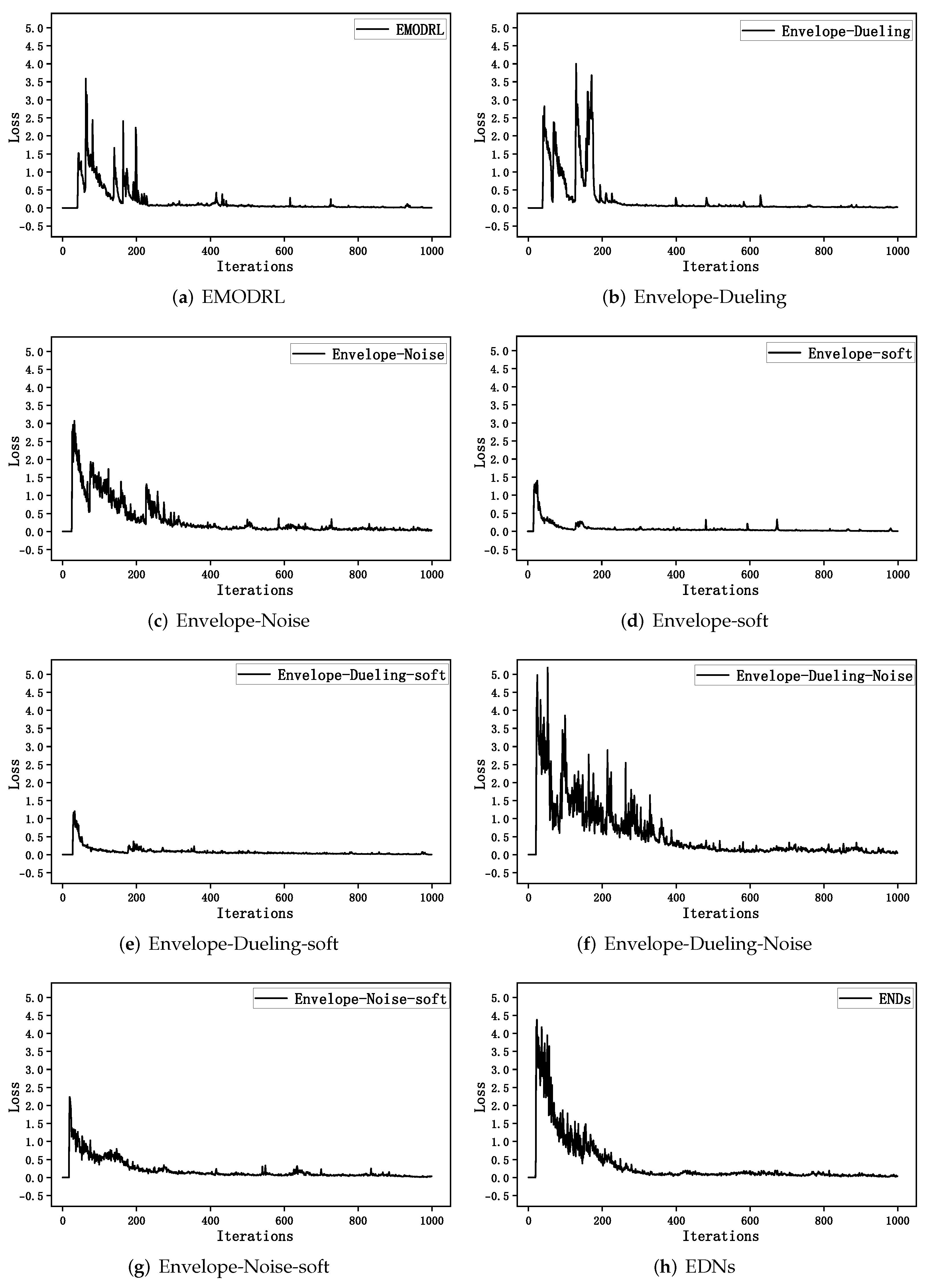
In this paper, the loss function curves of the EMODRL, envelope–dueling, envelope–noisy, envelope–soft, envelope–dueling–noise, envelope–noisy–soft, envelope–dueling–soft, and ENDs algorithms are compared with the number of training episodes as the horizontal coordinate and the loss function value as the vertical coordinate, and the performance of the above algorithms was analyzed according to the loss function curves. The experimental results are presented in Figure 4.
As can be seen from Figure 4a, the loss function of the EMODRL algorithm shows significant ups and downs in the pre-training period, because the agent does not explore the environment sufficiently at the beginning of the algorithm training phase, resulting in the behavioral values corresponding to individual states rarely being updated. When an agent reaches a state for the first time and receives a larger immediate reward, known from the behavioral value update formula, the network is updated significantly. Therefore, the calculated loss value is more extensive, which indicates that deviations in the initial value setting of the traditional ε -greedy strategy can significantly affect the exploration of the environment by the agent and, thus, lead to unsatisfactory algorithm training results. However, the exploration intensity can be adjusted by adjusting the size of ε , which is tedious and time-consuming. As shown in Figure 4b, the envelope–dueling algorithm introduces the dueling network structure based on the envelope update method. However, this approach fully considers that different behaviors can bring different advantages to the agent and bring certain speed and stability improvements. However, the loss function curve still has relatively clear ups and downs in the early stage. Because of the improved network structure and the behavioral value of the output is optimized, the exploration effort makes the overall performance of the algorithm training poor. This further illustrates the limitation of the ε -greedy strategy in different network structures. Looking at Figure 4c, it is apparent that the envelope–noise algorithm adds exploration noise into the parameters of the fully connected neural network layer. The loss function curve is less volatile. It shows a better convergence trend in the pre-training period than the EMODRL algorithm and the envelope–dueling algorithm. It indicates that adding exploration noise to the network can bring persistent, state-independent stochastic perturbations during network updates compared to the traditional ε -greedy strategy. It improves the efficiency of the agent exploration of the environment to some extent. As shown in Figure 4d, the envelope–soft algorithm introduces a soft update based on the envelope update method. The loss function curve decreases rapidly in the early stage, but there are still local fluctuations in the later stage. It is worth noting that since the soft update method updates the target network at each iteration using a convex combination of the behavioral and target networks, the update coefficient τ takes a smaller value. The loss function curve has an overall smaller loss value. The envelope–dueling–soft algorithm introduces both the dueling network and the soft update method, which inherits the advantages of the soft method. We can see from the loss function curve in Figure 4e that it decreases quickly in the early stage and the dueling structure makes the algorithm less volatile in the later stage. The envelope–dueling–noise algorithm inherits the advantages of the noise method, and the loss function curve is displayed in Figure 4f, which is less volatile in the pre-training period; the dueling structure makes the algorithm perform more stably in the later period. The envelope–noise–soft algorithm inherits the advantages of the noise and soft methods. The loss function curve is shown in Figure 4g, which in the early stage declines quickly and fluctuates less, but shows poor stability in the late training period.
Finally, from Figure 4h above, we can see that the envelope update method, dueling network, exploration noise, and soft update method are simultaneously fused into the MODRL algorithm to obtain the new MODRL algorithm EDNs, whose loss function curve decreases more smoothly during the training process and performs more stably in the later stage. EDNs has the best convergence speed and stable performance compared with the other algorithms.
In addition to analyzing the convergence performance of the algorithm from the loss function curve, we compared the performance based on two metrics, coverage ratio and adaptation error. The coverage ratio represents the ability of the agent to find the optimal solution on the ccs after the algorithm training, as shown in Equation (10).
CR ( F ) = 2 · precision · recall precision + recall
where the precision = F ccs / | F | , F is all solutions retrieved by the agent, and F ccs is the optimal solution for the agent, indicating the fraction of optimal solutions among the retrieved solutions. The recall = F ccs / | ccs | , indicating the fraction of optimal instances that have been retrieved over the total amount of optimal solutions. The adaptation error represents the gap between the retrieved control frontier and the theoretical optimal frontier and is used to measure the agent’s ability to adapt to the policy of the specified preference vector, when the agent is provided with a specific preference ω in the adaptation phase, as shown in Equation (11).
AE ( C ) = E ω D ω C ( ω ) C opt ( ω ) / C opt ( ω )
where the control frontier C π ω = ω T r ^ π ω and the optimal control frontier C opt : Ω R with ω max r ^ ccs ω T r ^ .
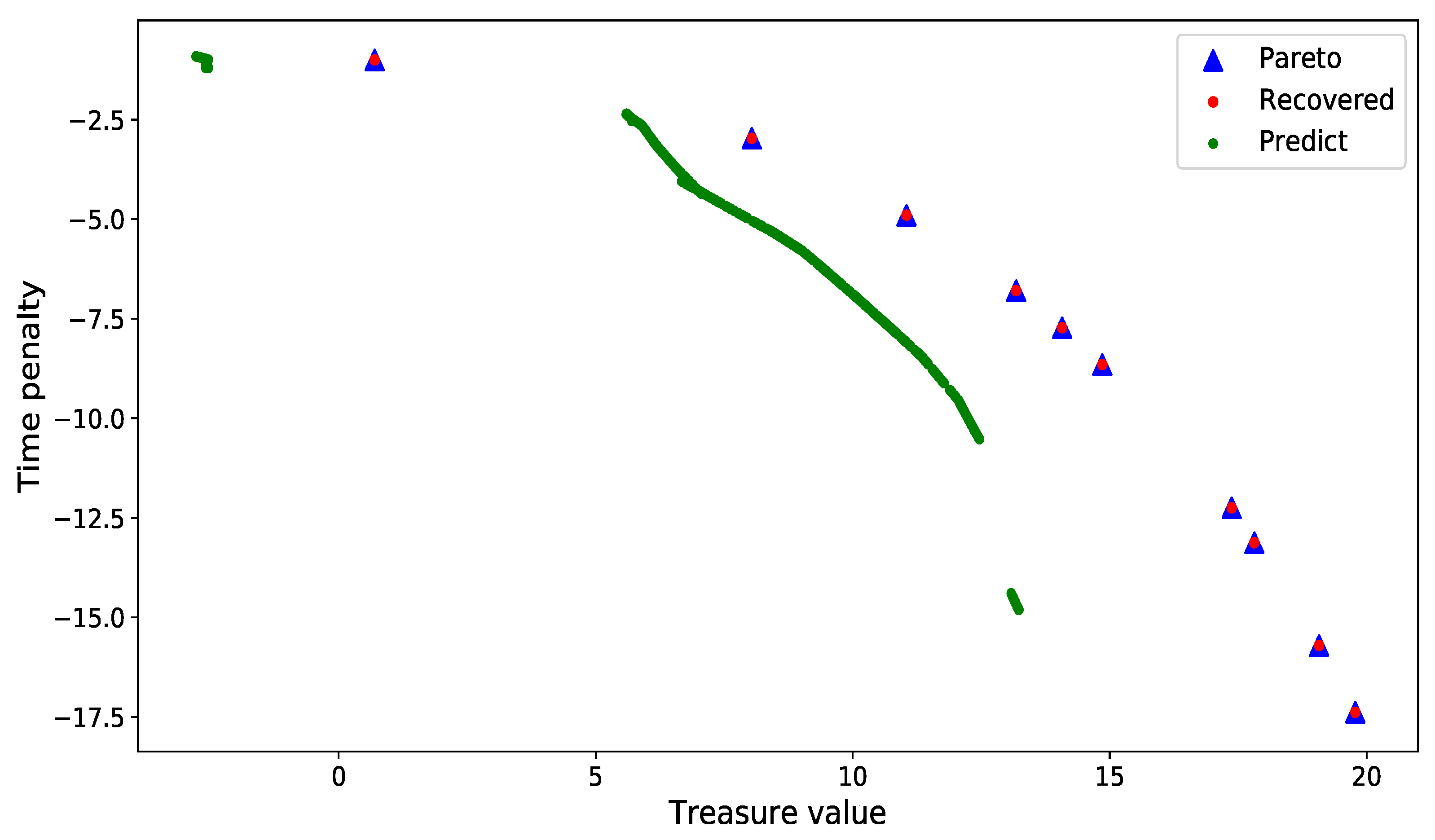
Based on the parameter settings in Table 1, we tested each algorithm’s coverage and adaptation error in the trained model, and the average of the coverage and adaptation error obtained from 10 tests was taken as the final result. The comparison results between different algorithms are provided in Table 2, and the coverage and adaptation errors of ENDs are shown in Figure 5. We can see from Figure 5 that the solution set found by the agent almost overlaps with the theoretical optimal frontier, which indicates that the agent has a good ability to find the optimal solution set. The difference between the predicted value and the theoretical optimal frontier is also small, which indicates that the agent has a good ability to adapt to the strategy of specifying the preference vector.
It can be seen from the data in Table 2 that, in 1000 episodes of testing, the EDNs algorithm performed best in coverage. Compared with the EMODRL algorithm, the coverage improved by 5.39%. The envelope–noise algorithm improved coverage by 2.53% compared to the EMODRL algorithm by adding noise to the weights of the fully connected layer of the network, which provides a higher exploration efficiency for the agent, allowing all states of behavioral values to be fully updated. The envelope–dueling algorithm introduces the dueling network structure, which fully considers that different behaviors can bring different advantages to the agent, improving the coverage rate by 1.16% compared to the EMODRL algorithm. The coverage rate of the envelope–soft algorithm is relatively low, probably because the target network is updated at each iteration, decreasing the stable agent. In addition, the envelope–dueling–noise, envelope–noise–soft, and envelope–dueling–soft algorithms all have some improvement in coverage.
The EDNs algorithm has a minor adaptation error compared with the EMODRL algorithm in measuring the ability of the agent to adapt to a specified preference vector, with a reduction of 36.87%. The adaptation errors of the envelope–soft, envelope–dueling–soft, and envelope–noise–soft algorithms are reduced compared to the EMODRL algorithm by 33.33%, 10.61%, and 20.71%, which also performs well, indicating that the soft update method performs well in improving the adaptation error of multi-objective deep reinforcement learning. However, the envelope–dueling, envelope–noise and envelope–dueling–noise algorithms perform poorly in terms of adaptive error, possibly due to the altered network structure or excessive action exploration.

6. Conclusions and Future Work

This paper proposes a novel MORL algorithm to address the problems of the insufficient exploration and unstable convergence of RL algorithms on high-dimensional multi-objective optimization. Firstly, the EDNs algorithm replaces the traditional DQN with a dueling network structure to make the agent have faster convergence speed. Secondly, the exploration noise is added to the fully connected layer of the network to improve the exploration efficiency of the agent, so that the agent has a stronger exploration ability and learns the optimal multi-objective strategy faster. Finally, a soft update method is used to update the target network parameters, which improves the convergence speed and stability of the agent. In the DST validation environment, the experimental results show that the EDNs algorithm has better stability and exploration ability and improves the coverage and adaptation error compared with the other algorithms. The following work will build on this research for nonlinear multi-objective reinforcement learning algorithms and continue to explore the effect of noise and exploration ability on the agent, aiming to find the fastest optimal equilibrium multi-objective strategy.

Author Contributions

Conceptualization, C.H.; methodology, C.H.; software, C.H.; validation, C.H., Z.Z. and C.Z.; formal analysis, C.H.; resources, C.H.; writing original draft preparation, C.H. and C.Z.; writing—review and editing, C.H. and C.Z.; visualization, C.H., Y.Y. and L.W.; supervision, Z.Z.; project administration, Z.Z.; funding acquisition, Z.Z. and C.Z. All authors have read and agreed to the published version of the manuscript.

Funding

Project supported by the Natural Science Foundation of the Higher Education Institutions of Jiangsu Province, China (Grant No. 22KJB520012), Key Research and Development Program (Applied Basic Research) of Changzhou, China (Grant No. CJ20210123), and Postgraduate Research Innovation Project of Jiangsu Province, China (Grant No. KYCX223053). Here, we would like to express our gratitude to them.

Conflicts of Interest

The authors declare no conflict of interest.

References

  1. Gronauer, S.; Diepold, K. Multi-agent deep reinforcement learning: A survey. Artif. Intell. Rev. 2022, 55, 895–943. [Google Scholar] [CrossRef]
  2. Pateria, S.; Subagdja, B.; Tan, A.H.; Quek, C. Hierarchical reinforcement learning: A comprehensive survey. ACM Comput. Surv. (CSUR) 2021, 54, 1–35. [Google Scholar] [CrossRef]
  3. Chen, W.; Qiu, X.; Cai, T.; Dai, H.N.; Zheng, Z.; Zhang, Y. Deep reinforcement learning for Internet of Things: A comprehensive survey. IEEE Commun. Surv. Tutor. 2021, 23, 1659–1692. [Google Scholar] [CrossRef]
  4. Czech, J. Distributed methods for reinforcement learning survey. In Reinforcement Learning Algorithms: Analysis and Applications; Springer: Berlin/Heidelberg, Germany, 2021; pp. 151–161. [Google Scholar]
  5. Schneider, S.; Khalili, R.; Manzoor, A.; Qarawlus, H.; Schellenberg, R.; Karl, H.; Hecker, A. Self-learning multi-objective service coordination using deep reinforcement learning. IEEE Trans. Netw. Serv. Manag. 2021, 18, 3829–3842. [Google Scholar] [CrossRef]
  6. Hayes, C.F.; Rădulescu, R.; Bargiacchi, E.; Källström, J.; Macfarlane, M.; Reymond, M.; Verstraeten, T.; Zintgraf, L.M.; Dazeley, R.; Heintz, F.; et al. A practical guide to multi-objective reinforcement learning and planning. Auton. Agents Multi-Agent Syst. 2022, 36, 26. [Google Scholar] [CrossRef]
  7. Nakayama, H.; Yun, Y.; Yoon, M. Sequential Approximate Multiobjective Optimization Using Computational Intelligence; Springer: Berlin/Heidelberg, Germany, 2010. [Google Scholar]
  8. Konak, A.; Coit, D.W.; Smith, A.E. Multi-objective optimization using genetic algorithms: A tutorial. Reliab. Eng. Syst. Saf. 2006, 91, 992–1007. [Google Scholar] [CrossRef]
  9. Friedman, E.; Fontaine, F. Generalizing across multi-objective reward functions in deep reinforcement learning. arXiv 2018, arXiv:1809.06364. [Google Scholar]
  10. Roijers, D.M.; Vamplew, P.; Whiteson, S.; Dazeley, R. A survey of multi-objective sequential decision-making. J. Artif. Intell. Res. 2013, 48, 67–113. [Google Scholar] [CrossRef] [Green Version]
  11. Dornheim, J. gTLO: A Generalized and Non-linear Multi-Objective Deep Reinforcement Learning Approach. arXiv 2022, arXiv:2204.04988. [Google Scholar]
  12. Andrychowicz, M.; Wolski, F.; Ray, A.; Schneider, J.; Fong, R.; Welinder, P.; McGrew, B.; Tobin, J.; Pieter Abbeel, O.; Zaremba, W. Hindsight experience replay. In Proceedings of the Advances in Neural Information Processing Systems 30: Annual Conference on Neural Information Processing Systems, Long Beach, CA, USA, 4–9 December 2017. [Google Scholar]
  13. Dubey, R.; Mishra, V.N. Higher-order symmetric duality in nondifferentiable multiobjective fractional programming problem over cone contraints. Stat. Optim. Inf. Comput. 2020, 8, 187–205. [Google Scholar] [CrossRef]
  14. Vandana, D.R.; Deepmala, M.L.; Mishra, V. Duality relations for a class of a multiobjective fractional programming problem involving support functions. Am. J. Oper. Res. 2018, 8, 294–311. [Google Scholar] [CrossRef] [Green Version]
  15. Vamplew, P.; Dazeley, R.; Berry, A.; Issabekov, R.; Dekker, E. Empirical evaluation methods for multiobjective reinforcement learning algorithms. Mach. Learn. 2011, 84, 51–80. [Google Scholar] [CrossRef] [Green Version]
  16. Van Moffaert, K.; Drugan, M.M.; Nowé, A. Scalarized multi-objective reinforcement learning: Novel design techniques. In Proceedings of the 2013 IEEE Symposium on Adaptive Dynamic Programming and Reinforcement Learning (ADPRL), Singapore, 16–19 April 2013; pp. 191–199. [Google Scholar]
  17. Vamplew, P.; Dazeley, R.; Foale, C. Softmax exploration strategies for multiobjective reinforcement learning. Neurocomputing 2017, 263, 74–86. [Google Scholar] [CrossRef] [Green Version]
  18. Abels, A.; Roijers, D.; Lenaerts, T.; Nowé, A.; Steckelmacher, D. Dynamic weights in multi-objective deep reinforcement learning. In Proceedings of the International Conference on Machine Learning (PMLR), Long Beach, CA, USA, 9–15 June 2019; pp. 11–20. [Google Scholar]
  19. Xu, J.; Tian, Y.; Ma, P.; Rus, D.; Sueda, S.; Matusik, W. Prediction-guided multi-objective reinforcement learning for continuous robot control. In Proceedings of the International Conference on Machine Learning (PMLR), Virtual, 13–18 July 2020; pp. 10607–10616. [Google Scholar]
  20. de Oliveira, T.H.F.; de Souza Medeiros, L.P.; Neto, A.D.D.; Melo, J.D. Q-Managed: A new algorithm for a multiobjective reinforcement learning. Expert Syst. Appl. 2021, 168, 114228. [Google Scholar] [CrossRef]
  21. Tajmajer, T. Modular multi-objective deep reinforcement learning with decision values. In Proceedings of the 2018 Federated Conference on Computer Science and Information Systems (FedCSIS), Poznan, Poland, 9–12 September 2018; pp. 85–93. [Google Scholar]
  22. Nguyen, T.T.; Nguyen, N.D.; Vamplew, P.; Nahavandi, S.; Dazeley, R.; Lim, C.P. A multi-objective deep reinforcement learning framework. Eng. Appl. Artif. Intell. 2020, 96, 103915. [Google Scholar] [CrossRef]
  23. Nguyen, N.D.; Nguyen, T.T.; Vamplew, P.; Dazeley, R.; Nahavandi, S. A Prioritized objective actor–critic method for deep reinforcement learning. Neural Comput. Appl. 2021, 33, 10335–10349. [Google Scholar] [CrossRef]
  24. Guo, K.; Zhang, L. Multi-objective optimization for improved project management: Current status and future directions. Autom. Constr. 2022, 139, 104256. [Google Scholar] [CrossRef]
  25. Monfared, M.S.; Monabbati, S.E.; Kafshgar, A.R. Pareto-optimal equilibrium points in non-cooperative multi-objective optimization problems. Expert Syst. Appl. 2021, 178, 114995. [Google Scholar] [CrossRef]
  26. Peer, O.; Tessler, C.; Merlis, N.; Meir, R. Ensemble bootstrapping for Q-Learning. In Proceedings of the International Conference on Machine Learning (PMLR), Virtual, 18–24 July 2021; pp. 8454–8463. [Google Scholar]
  27. Yang, R.; Sun, X.; Narasimhan, K. A generalized algorithm for multi-objective reinforcement learning and policy adaptation. In Proceedings of the Advances in Neural Information Processing Systems 32: Annual Conference on Neural Information Processing Systems, Vancouver, BC, Canada, 8–14 December 2019. [Google Scholar]
  28. Wang, Z.; Schaul, T.; Hessel, M.; Hasselt, H.; Lanctot, M.; Freitas, N. Dueling network architectures for deep reinforcement learning. In Proceedings of the International Conference on Machine Learning (PMLR), New York, NY, USA, 20–22 June 2016; pp. 1995–2003. [Google Scholar]
  29. Zhu, Z.; Hu, C.; Zhu, C.; Zhu, Y.; Sheng, Y. An improved dueling deep double-q network based on prioritized experience replay for path planning of unmanned surface vehicles. J. Mar. Sci. Eng. 2021, 9, 1267. [Google Scholar] [CrossRef]
  30. Treesatayapun, C. Output Feedback Controller for a Class of Unknown Nonlinear Discrete Time Systems Using Fuzzy Rules Emulated Networks and Reinforcement Learning. Fuzzy Inf. Eng. 2021, 13, 368–390. [Google Scholar] [CrossRef]
  31. Xu, H.; Zhang, C.; Wang, J.; Ouyang, D.; Zheng, Y.; Shao, J. Exploring parameter space with structured noise for meta-reinforcement learning. In Proceedings of the Twenty-Ninth International Conference on International Joint Conferences on Artificial Intelligence, Yokohama, Japan, 7–15 January 2021; pp. 3153–3159. [Google Scholar]
  32. Yang, T.; Tang, H.; Bai, C.; Liu, J.; Hao, J.; Meng, Z.; Liu, P. Exploration in deep reinforcement learning: A comprehensive survey. arXiv 2021, arXiv:2109.06668. [Google Scholar]
  33. Fortunato, M.; Azar, M.G.; Piot, B.; Menick, J.; Osband, I.; Graves, A.; Mnih, V.; Munos, R.; Hassabis, D.; Pietquin, O.; et al. Noisy networks for exploration. arXiv 2017, arXiv:1706.10295. [Google Scholar]
  34. Sokar, G.; Mocanu, E.; Mocanu, D.C.; Pechenizkiy, M.; Stone, P. Dynamic sparse training for deep reinforcement learning. arXiv 2021, arXiv:2106.04217. [Google Scholar]
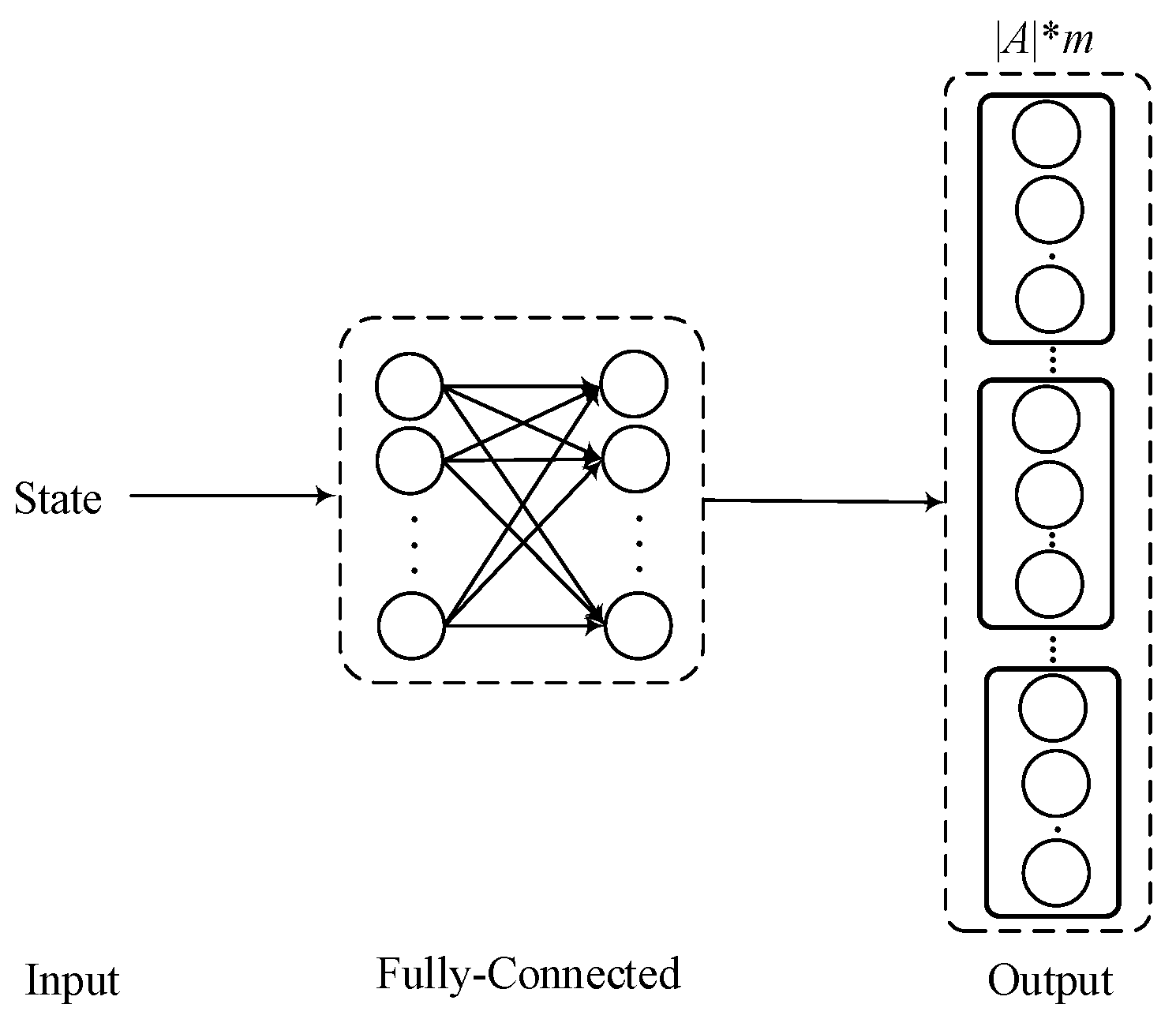
Figure 1. Standard MODRL framework. First, the agent takes the currently observed state as the input, then through two fully connected layers. Finally, it outputs n sets of optimization targets for action selection.
Electronics 11 02479 g001
Figure 2. Dueling MODRL framework. First, the agent takes as the input the observed state and preference vector, and then through two fully connected layers, the advantages of each action are fully considered through the dueling structure. Finally, the optimal action is output.
Electronics 11 02479 g002
Figure 3. Fully connected layer. p represents the number of inputs; q represents the number of outputs; w i j is the weight; b j is the bias term.
Electronics 11 02479 g003
Figure 4. Loss function curves between different algorithms.
Electronics 11 02479 g004
Figure 5. Coverage ratio and adaptation error of ENDs. The blue triangles represent the theoretical optimal frontier; the red dots represent the set of solutions found by the agent; the green dots represent the control frontier retrieved under the specified preference vector.
Electronics 11 02479 g005
Table 1. Parameter settings of the different algorithms.
AlgorithmLearning RateDiscount FactorSoft Update Factor
EMODRL0.0010.99/
Envelope–dueling0.0010.99/
Envelope–noise0.0010.99/
Envelope–soft0.0010.990.01
Envelope–dueling–soft0.0010.990.01
Envelope–dueling–noise0.0010.99/
Envelope–noise–soft0.0010.990.01
ENDs0.0010.990.01
Table 2. Comparison of coverage ratio and adaptation error among different algorithms.
AlgorithmCoverage RatioAdaptation Error
EMODRL94.7%0.198
Envelope–dueling95.8%0.338
Envelope–noise97.1%0.275
Envelope–soft91.4%0.132
Envelope–dueling–soft95.1%0.177
Envelope–dueling–noise98.2%0.414
Envelope–noise–soft96.3%0.157
ENDs99.8%0.125
Publisher’s Note: MDPI stays neutral with regard to jurisdictional claims in published maps and institutional affiliations.