Adaptive Fuzzy Observer Control for Half-Car Active Suspension Systems with Prescribed Performance and Actuator Fault

Abstract

In this paper, an adaptive fuzzy observer-based fault-tolerant controller is designed for a half-car active suspension system under the presence of uncertain parameters, unknown masses of passengers, and actuator failures. To improve the control performance, fuzzy logic systems (FLSs) are employed to approximate the unknown functions caused by uncertain dynamics of the suspension system. Then, an adaptive control design is developed to compensate for the effects of a non-ideal actuator. To improve passenger comfort, both vertical and angular motions are guaranteed simultaneously under the predefined boundaries by the prescribed performance function (PPF) method. Besides, the objectives of handling stability and driving safety are also considered to enhance the suspension performance. The system stability is proved according to the Lyapunov theory. Finally, the effectiveness of the developed approach is evaluated by comparative simulation examples on the half-car model. The simulation results show that the proposed control can improve the suspension performance as the RMS acceleration value is decreased by 68.1%.

1. Introduction

Vehicle suspension systems have received more attention both in the automobile industry and academic research since they provide passenger comfort and driving safety [1]. Although the active suspension system requires a flexible structure that is designed by an external actuator to create an active force, it has shown effectiveness in regulating the chassis displacement in comparison with passive or semi-active suspension [2]. Over the past decades, many types of actuators have been used for active suspensions, such as hydraulic [3], electromagnetic [4], or pneumatic devices [5], to dissipate the external excitation from road disturbance. However, precise modeling and control strategies to accurately monitor the vehicle performance in question have not been demonstrated. Besides, the damping and stiffness coefficients of active suspension are always nonlinear parameters, which can degrade the suspension performance if these problems are neglected.

To enhance ride comfort, many advanced control techniques have been designed for active suspension systems such as robust control [6], optimal control [7], output feedback control [8], sliding mode control [9], and backstepping control [10]. To stabilize the chassis displacement under the effect of external disturbance, Pan et al. [8] proposed an output feedback controller for the vehicle suspension which can efficiently compensate for unknown parameters. Although the time-delayed optimal control is investigated to guarantee the chassis stability by Yan et al. [7], the actuator dynamics were not investigated to fully consider the requirements of the suspension system. To enhance the suspension performance under the effect of actuator fault and unmodeled parameters, Kazemipour et al. [11] designed a novel terminal sliding mode controller which can enhance the finite-time convergence of tracking error of chassis movement. Besides, Pusadkar et al. [12] proposed an adaptive sliding mode based on linear disturbance observer for a quarter car model to overcome external disturbance and a non-ideal actuator. However, the problems of chattering and singularity in the control law are possible limitations associated with the SMC technique. To improve passenger comfort and guarantee the suspension displacement, an adaptive backstepping technique was proposed by Pang et al. [13]. Nonetheless, most previous studies focused on enhancing the passenger comfort for the quarter car model, which cannot ensure the pitch motion of the chassis. Furthermore, the objectives of driving safety and handling stability need to be considered continuously, which can be designed for practical application.

On the other hand, most suspension control methods that have been developed based on the system modeling are exactly known while parametric uncertainties are ignored. However, these assumptions rarely occur since vehicle suspension contains uncertain parameters which can degrade the control performance. To overcome these above limitations, some intelligent control algorithms are employed to compensate for unknown functions including fuzzy logic systems [14] and neural networks [15]. In order to approximate external disturbances and uncertain parameters, Zhang et al. [16] proposed a neural network-based adaptive dynamic surface controller for an active seat suspension model. Li et al. [17] designed a fuzzy finite-frequency output feedback control to estimate the uncertainties of vehicle suspension which can guarantee the suspension performance under the effect of time delay and output constraints. Besides, the problem of the uncertain suspension model was investigated by the fuzzy logic approach based on the dynamic sliding-mode method to improve passenger comfort [18]. However, the actuator dynamic was often neglected in the system modeling, which can lead to system instability. In addition, some problems’ actuator failures were not taken seriously in most previous studies of active suspension.

Generally, many control laws have been developed for active suspension systems to enhance passenger comfort by reducing the chassis displacement without considering the output constraint of sprung mass motion. Unfortunately, the convergence rate of tracking error strongly affects the control performance since it may lead to handling instability and degrade the driving safety if the displacement constraint is violated. For this purpose, a novel output constraint called prescribed performance was developed by Bechlioulis et al. to guarantee the maximum overshoot of tracking error within a small boundary [19]. With the PPF technique, many controllers have been designed to satisfy the tracking accuracy and improve the system stability [20,21]. To stabilize the chassis displacement, an adaptive controller was designed for the active suspension, considering the unknown nonlinear dynamics, to improve the ride comfort and guarantee driving safety. Huang et al. [22] proposed a novel control strategy that can ensure the steady-state response of the active suspension by applying a prescribed performance function. Similarly, to guarantee the convergence rate of the vehicle suspension system, an adaptive control-based prescribed performance technique was developed by Na et al. [23] which can compensate for the unknown nonlinearities. However, a few studies applied the PPF constraint for the half-car active suspension to guarantee the convergence rate of vertical displacement and pitch motions simultaneously, which motivates this research.

The problem of actuator failure has not been seriously considered in most of the previous works for vehicle suspension systems. Instead, many proposed controllers assume that the ideal actuators are used to dissipate external vibration even though the non-smooth nature of actuator failure can destroy the suspension performance [24]. To improve the control efficiency and ensure system stability, the issue of fault-tolerant control should be investigated for vehicle suspension [25,26,27]. Liu et al. [28] proposed an adaptive fault-tolerant control problem to stabilize vehicle suspension under the effect of unknown actuator failures. To improve passenger comfort, Liu et al. [29] designed an adaptive sliding fault-tolerant controller for the vehicle suspension system considering the issues of actuator faults and parameter uncertainties. Note that all mentioned studies focused on error compensation for an actuator failure quarter car model and ignored the tracking constraint of sprung mass displacement. Therefore, ensuring the vertical and pitch motions of the half-car suspension model under the effects of actuator failures and unknown parameters still presents challenges in vehicle suspension design.

Inspired by the above discussions, we propose an adaptive control for a half-car active suspension system considering the unknown functions and actuator failure problem. With the PPF technique, the chassis displacement and angular motion are guaranteed simultaneously to enhance passenger comfort. Besides, the objectives of handling stability and driving safety are satisfied by the dynamic analysis. The major advantages of this work are summarized as follows.

1.

The half-car active suspension is analyzed in the presence of uncertain parameters and actuator failures to guarantee ride comfort, suspension deflection, and driving safety;

2.

FLSs are applied to approximate the unknown functions of parametric uncertainties and different masses of passengers. Then, the adaptive fault-tolerant control is designed to compensate for the actuator fault problem;

3.

The PPF technique is incorporated into the control technique to constrain chassis displacement and angular motion within the small boundaries.

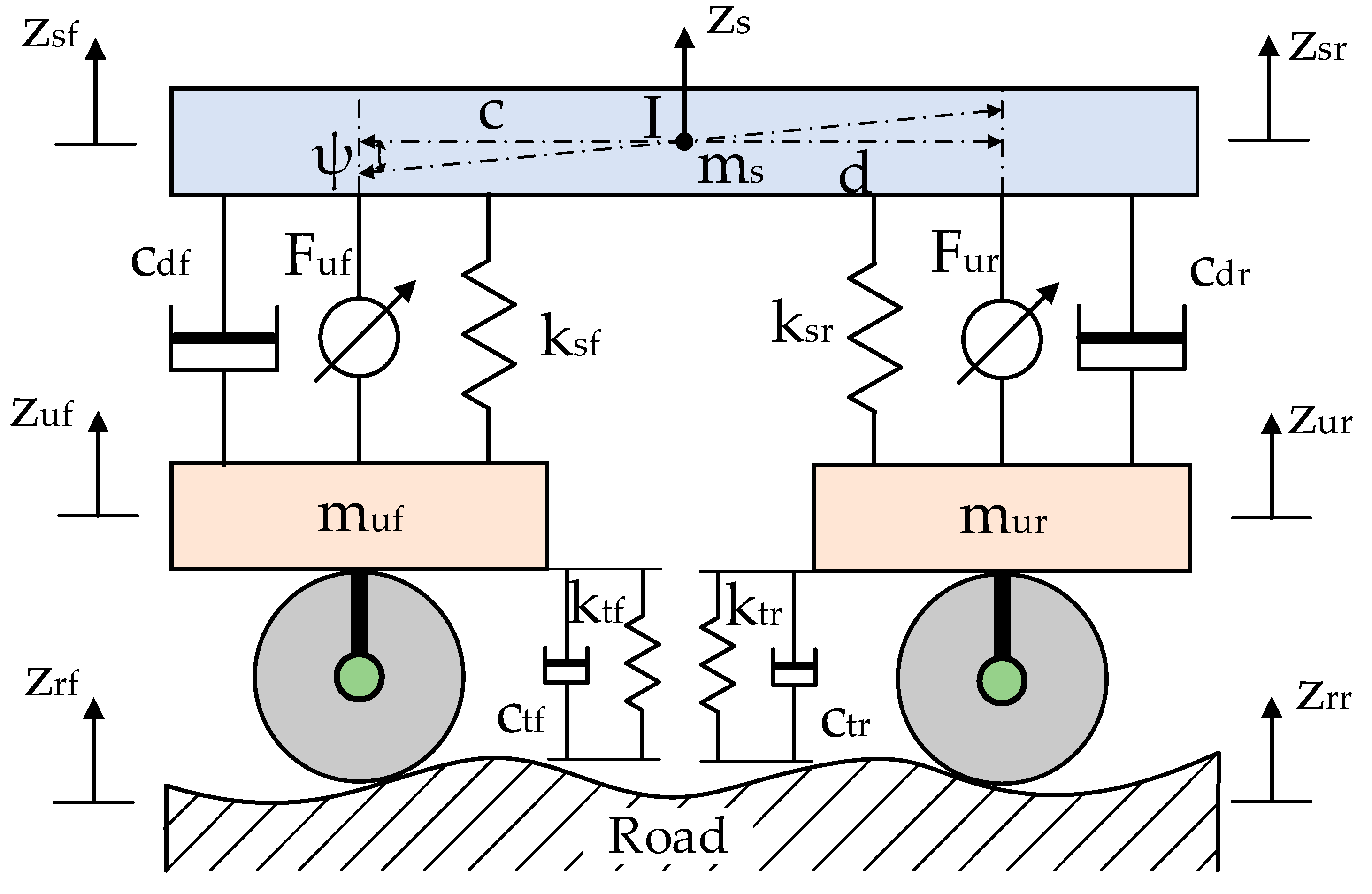
2. System Description

2.1. Half Car Suspension Model

The structure of the vehicle half-car model is displayed in Figure 1, consisting of one sprung mass, two unsprung masses at front and rear positions, two sets of mechanical springs and damping components, two active actuators, and two tire models. The total mass of the chassis and passenger are denoted by sprung mass while the unsprung mass represents the mechanical structure of the wheel and suspension frame. One set of a spring, a damper, and an actuator are installed between sprung mass and on unsprung mass. The tire is molded by one mechanical spring and damper. The irregular road roughness impacts the front and rear unsprung mass which causes external excitations to the passengers. The active suspension is designed to achieve passenger comfort by dissipating the continuous vibration with two active actuators. The mechanical equation of the half-car active suspension model can be expressed by:

$$\begin{array}{l}{m}_s{\ddot{z}}_s=-F_{sf}-F_{sr}-F_{df}-F_{dr}+F_v\\ I\ddot{\psi }=c\left(F_{sf}+F_{df}\right)-d\left(F_{sr}+F_{dr}\right)+F_{\psi }\\ m_{uf}{\ddot{z}}_{uf}=-F_{tf}-F_{cf}+F_{sf}+F_{df}-F_{uf}\\ m_{ur}{\ddot{z}}_{ur}=-F_{tr}-F_{cr}+F_{sr}+F_{dr}-F_{ur}\end{array}$$

(1)

where $m_s$ is the total weight while $I$ denotes the inertia of sprung mass; the front and rear unsprung masses are defined by $m_{uf}$ and $m_{ur}$, respectively; $z_s,z_{uf},z_{ur}$ represent the positions of sprung mass, front and rear unsprung masses, respectively; the structural length of the front and rear suspension are defined by $c$ and $d$ while the front and rear road profile are denoted by $z_{rf}$ and $z_{rr}$. The active forces of front and rear actuators are defined by $F_{uf}$ and $F_{ur}$. Then, the detailed forces for regulating the vertical and pitch motions $F_v$, $F_{\psi }$ are expressed as follows:

$$\begin{array}{l}{F}_v=F_{uf}+F_{ur}\\ F_{\psi }=d{F}_{ur}-c{F}_{uf}\end{array}$$

(2)

The dynamics forces of front and rear mechanical spring are described by $F_{sf}=k_{sf}(z_s-d\mathit{sin}\psi -z_{uf})$, $F_{df}=c_{df}({\dot{z}}_s-d\mathit{cos}\psi -{\dot{z}}_{uf})$, while the detailed damping forces are calculated by $F_{sr}=k_{sr}(z_s+c\mathit{sin}\psi -z_{ur})$, $F_{dr}=c_{dr}({\dot{z}}_s+c\mathit{cos}\psi -{\dot{z}}_{ur})$. Similarly, the spring and damping forces of front and rear tire models are expressed by $F_{tf}=k_{tf}(z_{uf}-z_{rf})$, $F_{cf}=c_{tf}({\dot{z}}_{uf}-{\dot{z}}_{rf})$, $F_{tr}=k_{tr}(z_{ur}-z_{rr})$, $F_{cr}=c_{tr}({\dot{z}}_{ur}-{\dot{z}}_{rr})$, in which $k_{sf}$ and $k_{sr}$ are the spring coefficients at the front and rear suspension; $c_{df}$ and $c_{dr}$ are the damping coefficients of the front and rear damping components.

Define the system state variables as $x_1=z_s$, $x_2={\dot{z}}_s$, $x_3=\psi$, $x_4=\dot{\psi }$, $x_5=z_{uf}$, $x_6={\dot{z}}_{uf}$, $x_7=z_{uf}$, and $x_8={\dot{z}}_{ur}$; the state-space form of the half-car suspension model (1) can be rewritten as follows:

$$\begin{array}{l}{\dot{x}}_1=x_2\\ {\dot{x}}_2=\frac{1}{m_s}\left(F_v-F_{sf}-F_{df}-F_{sr}-F_{dr}\right)\\ {\dot{x}}_3=x_4\\ {\dot{x}}_4=\frac{1}{I}\left(F_{\psi }+c\left(F_{sf}+F_{df}\right)-d\left(F_{sr}+F_{dr}\right)\right)\\ {\dot{x}}_5=x_6\\ {\dot{x}}_6=\frac{1}{m_{uf}}\left(-F_{uf}-F_{tf}-F_{cf}+F_{sf}+F_{df}\right)\\ {\dot{x}}_7=x_8\\ {\dot{x}}_8=\frac{1}{m_{ur}}\left(-F_{ur}-F_{tr}-F_{cr}+F_{sr}+F_{dr}\right)\end{array}$$

(3)

2.2. Actuator Fault Formulation and Preliminaries

Although many control schemes have been designed to improve suspension performance, the ideal actuators are considered in most vehicle systems. The unknown parameters and actuator faults are often unavoidable in practical applications, which can degrade the system’s stability. Hence, the fault tolerance problem should be investigated in the control design to evaluate the actual system dynamics. For this purpose, two types of actuator failures are considered in this research, that is, the lock-in-place model and the loss of effectiveness definition.

(1)

Lock-in-place type: In this case, the actuator is stuck and cannot respond to the input control signal. Then, the actual signal can be described by $F_v={\varphi }_v$ and $F_{\psi }={\varphi }_{\psi }$, in which ${\varphi }_v$ is the constant values of the float fault of $F_v$ and ${\varphi }_w$ is the constant values of the float fault of $F_{\psi }$.

(2)

Loss of effectiveness model: The actual control cannot satisfy the complete value of signal control in this case. This means that some effectiveness is lost, which is denoted by the coefficient factor ${\mu }_v$ and ${\mu }_{\psi }$. For example, ${\mu }_v=0.6$ indicates that the remaining coefficient actuator is $60\%$ while the loss signal of the vertical control actuator is $40\%$.

Therefore, the two actuator failure cases can be described in general forms:

$$\begin{array}{l}{F}_v={\mu }_v{F}_v^{\ast }+{\varphi }_v\\ F_{\psi }={\mu }_{\psi }{F}_{\psi }^{\ast }+{\varphi }_{\psi }\end{array}$$

(4)

where $F_v^{*}$ and $F_{\psi }^{*}$ denote the ideal actuator signal.

Since the spring and damping coefficients and passenger masses are not exactly determined in actual system modeling, the vehicle half-car suspension contains unknown functions which cannot be applied to the control design process. To overcome this drawback, FLSs can be used as a good estimation technique in this study. An FLS combines four individual parts; they are a knowledge rule base, a fuzzifier, a fuzzy inference engine, and a defuzzifier. The FLSs knowledge base includes a series of fuzzy rules, “If–Then”, as follows:

$$R^k: \mathrm{If} x_1 \mathrm{is} G_1^k \mathrm{and} x_2 \mathrm{is} G_2^k \mathrm{and} \dots x_n \mathrm{is} G_n^k, \mathrm{then} y \mathrm{is} H^k, k=1,\hspace{0.17em}\dots \hspace{0.17em},N$$

(5)

where $X={[x_1,x_2,\hspace{0.17em}\dots \hspace{0.17em},x_n]}^T$ is FLSs input of a system variable and $y$ is the output value; $G_i^k$ and $H^k$ represent fuzzy sets corresponding to membership functions ${\chi }_{G_i^k}\left(x_i\right)$ and ${\chi }_{H^k}\left(y\right)$; and $N$ is the number of fuzzy rules [30].

Therefore, the FLSs can be described via singleton fuzzifier, center average defuzzification, and product inference as follows:

$$y\left(X\right)=\frac{{\displaystyle {\sum }_{k=1}^N{\overline{y}}_k{\displaystyle {\prod }_{i=1}^n{\chi }_{G_i^k}\left(X_i\right)}}}{{\displaystyle {\sum }_{k=1}^N\left({\displaystyle {\prod }_{i=1}^n{\chi }_{G_i^k}\left(X_i\right)}\right)}}$$

(6)

where ${\overline{y}}_k=\underset{y\in R}{max}\left\{{\chi }_{H^k}\left(y\right)\right\}$.

Define fuzzy basis functions as:

$$s_k\left(X_i\right)=\frac{{\displaystyle {\prod }_{i=1}^n{\chi }_{G_i^k}\left(X_i\right)}}{{\displaystyle {\sum }_{k=1}^N\left({\displaystyle {\prod }_{i=1}^n{\chi }_{G_i^k}\left(X_i\right)}\right)}}$$

(7)

Let $S(X)={[s_1(X),s_2(X),\hspace{0.17em}\dots \hspace{0.17em},s_N(X)]}^T$ and ${\theta }^T=[{\overline{y}}_1,{\overline{y}}_2,\hspace{0.17em}\dots \hspace{0.17em},{\overline{y}}_N]=[{\theta }_1,{\theta }_2,\hspace{0.17em}\dots \hspace{0.17em},{\theta }_N]$, we can write the fuzzy logic system (7) as:

$$y\left(X\right)={\theta }^{T}S\left(X\right)$$

(8)

Lemma 1

([31]). For any continuous unknown function $f\left(X\right)$ determined on a compact set $\Phi$. Then, for any given positive constant $\epsilon >0$ , there exist fuzzy logic systems ${\theta }^{T}S(X)$ that satisfy

$$\underset{X\in \Phi }{\mathit{sup}}\left|f\left(X\right)-{\theta }^{T}S\left(X\right)\right|\le \epsilon$$

(9)

where$\theta$is the ideal FLSs weight matrix, and$S\left(X\right)$is bounded by$\Vert S\left(X\right)\Vert \le \tau$.

In the control design in this study, the FLSs are used to approximate the unknown functions $f\left(X\right)$ with $X\in \Phi$:

$$f_i\left(X\right)={\theta }_i^T{S}_i\left(X_i\right)+{\eta }_i$$

(10)

In this study, the fuzzy “If-Then” rules are proposed as:

$$\begin{array}{c}{R}^1: \mathrm{If} x_1 \mathrm{is} H_1^1,x_2 \mathrm{is} H_2^1, \mathrm{and} x_3 \mathrm{is} H_3^1 \mathrm{then} y \mathrm{is} T^1\\ R^2: \mathrm{If} x_1 \mathrm{is} H_1^2,x_2 \mathrm{is} H_2^2, \mathrm{and} x_3 \mathrm{is} H_3^2 \mathrm{then} y \mathrm{is} T^2\\ R^3: \mathrm{If} x_1 \mathrm{is} H_1^3,x_2 \mathrm{is} H_2^3, \mathrm{and} x_3 \mathrm{is} H_3^3 \mathrm{then} y \mathrm{is} T^3\\ R^4: \mathrm{If} x_1 \mathrm{is} H_1^4,x_2 \mathrm{is} H_2^4, \mathrm{and} x_3 \mathrm{is} H_3^4 \mathrm{then} y \mathrm{is} T^4\\ R^5: \mathrm{If} x_1 \mathrm{is} H_1^5,x_2 \mathrm{is} H_2^5, \mathrm{and} x_3 \mathrm{is} H_3^5 \mathrm{then} y \mathrm{is} T^5\end{array}$$

when fuzzy sets are selected as $H_1^1=\left(NL\right)$, $H_2^1=\left(NL\right)$, $H_3^1=\left(NL\right)$, $H_1^2=\left(NS\right)$, $H_2^2=\left(NS\right)$, $H_3^2=\left(NS\right)$, $H_1^3=\left(ZE\right)$, $H_2^3=\left(ZE\right)$, $H_3^3=\left(ZE\right)$, $H_1^4=\left(PS\right)$, $H_2^4=\left(PS\right)$, $H_3^4=\left(PS\right)$, $H_1^5=\left(PL\right)$, $H_2^5=\left(PL\right)$, $H_3^5=\left(PL\right)$, which are defined over the interval [−2, 2] for variables $x_1$, $x_2$, and $x_3$ respectively. NL represents negative large, NS represents negative small, ZE represents zero, PS represents positive small, PL represents positive large, and choose −2, −1, 0, 1, 2 as center points.

Fuzzy membership functions (as shown in Figure 2) are defined as:

$$\begin{array}{l}{\mu }_{H_1^l}\left(x_1\right)=exp\left[-\frac{{\left(x_1-3+l\right)}^2}{4}\right]\\ {\mu }_{H_2^l}\left(x_2\right)=exp\left[-\frac{{\left(x_2-3+l\right)}^2}{4}\right]\\ {\mu }_{H_3^l}\left(x_3\right)=exp\left[-\frac{{\left(x_3-3+l\right)}^2}{4}\right]\end{array}$$

(11)

where $l=1,\hspace{0.17em}\dots \hspace{0.17em},\hspace{0.17em}5$.

To enhance the ride comfort, the control algorithm is designed to deplete the external road vibration by reducing the chassis displacement. However, improving the ride comfort requires larger suspension deflection. Due to the suspension design being limited by the mechanical structure, the control design must satisfy the three suspension objectives as follows:

(1)

Ride comfort: The chassis movement must be stabilized and isolated from the external violation of road disturbance, which can improve the passenger comfort;

(2)

Handling stability: The active suspension must guarantee the suspension deflection within the mechanical structure. To meet this requirement, the relative suspension deflection (RSD) has to be smaller than 1.

$$RSD=\frac{\left(z_s+dsin\psi -z_{uf}\right)}{z_M}$$

(12)

where $z_M$ is the maximum vertical displacement of the chassis.

(3)

Driving safety: This objective is considered to ensure that the tire should always contact with the road profile. For this purpose, the relative tire fore (RTF) must be kept less than 1.

$$RTF=\frac{F_{tf}+F_{cf}+F_{tr}+F_{cr}}{\left[m_s+m_{uf}+m_{ur}\right]g}$$

(13)

Remark 1.

Most of the previous suspension studies are proposed to improve the three above objectives. Nonetheless, increasing the ride comfort will enlarge the suspension stability, and even degrade the contact condition between tire and road surface. Besides, it requires regulating the active force at front and rear positions to stabilize the pitch motion of the half-car suspension model, which can overcome the actuator capacity. In this study, these objects can be guaranteed under the presence of actuator failures.

3. Adaptive Fuzzy Observer Control with Prescribed Performance

3.1. Prescribed Performance Function

This section employs the prescribed performance technique to limit the tracking error of the system state within the predefined boundary. First, define the tracking error by:

$$e=x-x_d$$

(14)

where $x_d$ is the desired trajectory.

A positive decreasing smooth function is used to describe the prescribed performance function as [19]:

$$\delta \left(t\right)=\left({\delta }_0-{\delta }_{\infty }\right)e^{-\gamma t}+{\delta }_{\infty }$$

(15)

where $\gamma >0$ denotes the convergence rate, ${\delta }_0$ is the initial value that is selected to meet two initial conditions:

$$\underset{t\to 0}{lim}\delta \left(t\right)={\delta }_0>0, \underset{t\to \infty }{lim}\delta \left(t\right)={\delta }_{\infty }>0, {\delta }_0>{\delta }_{\infty }$$

Then, the following inequality can be used to describe the constraint condition of the tracking error based on the prescribed performance:

$$-\underset{\_}{\beta }\delta \left(t\right)<e<\overline{\beta }\delta \left(t\right) t>0$$

(16)

where $\underset{\_}{\beta },\overline{\beta }>0$ are the lower and upper control parameters. Hence, the lower bound and upper bound of tracking error are determined by $-\underset{\_}{\beta }\delta (0)$ and $\overline{\beta }\delta (0)$, respectively. The inequality (16) can be guaranteed by selecting these positive parameters $\underset{\_}{\beta },\overline{\beta },{\delta }_0,{\delta }_{\infty },\gamma$.

However, the above inequality constraint cannot be directly applied to the controller design. Instead, it needs to transform the inequality condition of the tracking error into an equivalent unrestricted form. Hence, a smooth and strictly increasing function $Q\left(z\right)$ can be applied to this requirement:

$$Q\left(z\right)=\frac{\overline{\beta }{e}^z-\underset{\_}{\beta }{e}^{-z}}{e^z+e^{-z}}$$

(17)

Based on (16) and (17), we can express the equivalent unconstrained by:

$$e=\delta \left(t\right)Q\left(z\right)$$

(18)

By choosing the PPF parameter to satisfy the initial condition $\delta \left(t\right)>{\delta }_{\infty }>0$, the strictly monotonically increasing function $Q\left(z\right)$ can be rewritten by the inverse transfer function:

$$z=Q^{-1}\left(e/\delta \left(t\right)\right)$$

(19)

Therefore, the transform function of $z$ can be converted by the following equation:

$$z=\frac{1}{2}ln\left(\frac{\eta +\underset{\_}{\beta }}{\overline{\beta }-\eta }\right)-\frac{1}{2}ln\frac{\underset{\_}{\beta }}{\overline{\beta }}$$

(20)

where $\eta =e/\delta \left(t\right)$.

Lemma 2

([32]). By transforming the tracking error $e$ into a smooth function (17), it will be guaranteed within the small boundary of the prescribed performance (15).

Since the control parameters ${\delta }_0$, $\overline{\beta }$, $\overline{\beta }$ are selected to satisfy the initial condition $-\underset{\_}{\beta }\delta (0)<x(0)<\overline{\beta }\delta (0)$, the transform variable $z$ can be kept within the boundaries. Hence, the condition $-\underset{\_}{\beta }<Q(z)<\overline{\beta }$ is held while the constraint condition of tracking error $-\underset{\_}{\beta }\delta \left(t\right)<e<\overline{\beta }\delta \left(t\right)$ is ensured.

3.2. Adaptive Fuzzy Observer Controller with Prescribed Performance

To stabilize sprung mass movement, the control design will focus on the dynamic equation for sprung mass as follows:

$$\begin{array}{l}{\dot{x}}_1=x_2\\ {\dot{x}}_2=\frac{1}{m_s}\left(F_v-F_{sf}-F_{df}-F_{sr}-F_{dr}\right)\\ {\dot{x}}_3=x_4\\ {\dot{x}}_4=\frac{1}{I}\left(F_{\psi }+c\left(F_{sf}+F_{df}\right)-d\left(F_{sr}+F_{dr}\right)\right)\end{array}$$

(21)

Then, the tracking errors of vertical displacement and pitch motion are defined by

$$\begin{array}{l}{e}_1=x_1-x_{d1}\\ e_2=x_3-x_{d2}\end{array}$$

(22)

where $x_{d1}$ and $x_{d2}$ are the reference trajectory of vertical and angular motions, respectively.

Step 1: Propose the control signal $F_v^{\ast }$ for the vertical motion.

Choose the prescribed performance ${\delta }_1\left(t\right)=\left({\delta }_{01}-{\delta }_{\infty 1}\right)e^{-{\gamma }_{1}t}+{\delta }_{\infty 1}$. Based on (20), the transformed function for the tracking error of vertical displacement $z_1$ can be expressed as:

$$z_1=\frac{1}{2}ln\left(\frac{{\eta }_1+{\underset{\_}{\beta }}_1}{{\overline{\beta }}_1-{\eta }_1}\right)-\frac{1}{2}ln\frac{{\underset{\_}{\beta }}_1}{{\overline{\beta }}_1}$$

(23)

where ${\eta }_1=e_1/{\delta }_1\left(t\right)$.

Then, the time derivative of $z_1$ is obtained by:

$${\dot{z}}_1={\xi }_1\left(x_2-\frac{x_1{\dot{\delta }}_1}{{\delta }_1^2}\right)$$

(24)

where ${\xi }_1=\frac{1}{2{\delta }_1}\left(\frac{1}{{\eta }_1+{\underset{\_}{\beta }}_1}-\frac{1}{{\eta }_1-{\overline{\beta }}_1}\right)$.

Based on the transformed error $z_1$, the sliding surface $h_1$ is designed as follows:

$$h_1={\kappa }_1{z}_1+{\dot{z}}_1$$

(25)

where ${\kappa }_1$ is the positive design parameter.

The time derivative $h_1$ can be obtained by:

$${\dot{h}}_1=\frac{{\mu }_v}{m_s}\left[{\xi }_1{F}_v^{*}-\left(F_{sf}+F_{df}+F_{sr}+F_{dr}\right)+F_v\left(X_v\right)\right]$$

(26)

where

$$\begin{array}{r}{F}_v\left(X_v\right)=\frac{1}{{\mu }_v}{m}_s\left({\kappa }_1{\xi }_1+{\dot{\xi }}_1\right)\left(x_2-x_1\frac{{\dot{\delta }}_1}{{\delta }_1}\right)+{\xi }_1\frac{{\varphi }_v}{{\mu }_v}-\frac{1}{{\mu }_v}{m}_s\left(x_2\frac{{\dot{\delta }}_1}{{\delta }_1}+x_1\frac{{\ddot{\delta }}_1}{{\dot{\delta }}_1}-x_1\frac{{\dot{\delta }}_1^2}{{\dot{\delta }}_1^2}\right)\\ +\left(1-\frac{{\xi }_1}{{\mu }_v}\right)\left(F_{sf}+F_{df}+F_{sr}+F_{dr}\right)\end{array}$$

(27)

Based on Equation (27), the unknown function $F_v\left(X_v\right)$ contains the effectiveness factors of actuator failures ${\mu }_v$ and ${\varphi }_v$ that cannot be determined. The mass of passengers is an uncertain parameter, which cannot be applied to the control design. Under the effects of these problems, the suspension performance will be degraded and the system will become unstable. Hence, the FLSs can be employed as an approximation technique to develop the control algorithm. Based on Equation (10), the unknown function $F_v\left(X_v\right)$ can be estimated by:

$$F_v\left(X_v\right)={\theta }_v^T{S}_v\left(X_v\right)+{\eta }_v$$

(28)

where X_v = [x₁, x₂]^T denotes the input vector, ${\eta }_v$ illustrates the approximation error.

Then, we can rewrite the time derivative $h_1$ (26) as follows:

$${\dot{h}}_1=\frac{{\mu }_v}{m_s}\left[{\xi }_1{F}_v^{*}-\left(F_{sf}+F_{df}+F_{sr}+F_{dr}\right)+{\theta }_v^T{S}_v\left(X_v\right)+{\eta }_v\right]$$

(29)

From (29), the adaptive control law is designed,

$$F_v^{*}=\frac{1}{{\xi }_1}\left(\left(F_{sf}+F_{sr}+F_{df}+F_{dr}\right)-{\widehat{\theta }}_v^T{S}_v\left(X_v\right)-k_1{h}_1\right)$$

(30)

where $k_1>0$ is the control parameter.

The adaptive law can be proposed by:

$${\dot{\widehat{\theta }}}_v={\varsigma }_v\left[h_1{S}_v\left(X_v\right)-{\rho }_v{\widehat{\theta }}_v\right]$$

(31)

where ${\varsigma }_v$ and ${\rho }_v$ are the positive design parameters.

Step 2: Design the control $F_{\psi }^{*}$ for angular displacement.

Firstly, the transform function of $z_2$ can be obtained from (20):

$$z_2=\frac{1}{2}ln\left(\frac{{\eta }_2+{\underset{\_}{\beta }}_2}{{\overline{\beta }}_2-{\eta }_2}\right)-\frac{1}{2}ln\frac{{\underset{\_}{\beta }}_2}{{\overline{\beta }}_2}$$

(32)

where the prescribed performance is chosen by ${\delta }_2\left(t\right)=\left({\delta }_{02}-{\delta }_{\infty 2}\right)e^{-{\gamma }_{2}t}+{\delta }_{\infty 2}$ and we define ${\eta }_2=e_2/{\delta }_2\left(t\right)$.

The time derivative of $z_2$ can be obtained as follows:

$${\dot{z}}_2={\xi }_2\left(x_4-\frac{x_3{\dot{\delta }}_2}{{\delta }_2^2}\right)$$

(33)

where ${\xi }_2=\frac{1}{2{\delta }_2}\left(\frac{1}{{\eta }_2+{\underset{\_}{\beta }}_2}-\frac{1}{{\eta }_2-{\overline{\beta }}_2}\right)$.

Then, the sliding surface $h_2$ is determined by:

$$h_2={\kappa }_2{z}_2+{\dot{z}}_2$$

(34)

where ${\kappa }_2$ is the positive design parameter.

Hence, we can express the time derivative of $h_2$ as follows:

$${\dot{h}}_2=\frac{{\mu }_{\psi }}{I}\left[{\xi }_2{F}_{\psi }^{*}+c\left(F_{sf}+F_{df}\right)-d\left(F_{sr}+F_{dr}\right)+F_{\psi }\left(X_{\psi }\right)\right]$$

(35)

where

$$\begin{array}{r}{F}_{\psi }\left(X_{\psi }\right)=\frac{1}{{\mu }_{\psi }}I\left({\kappa }_2{\xi }_2+{\dot{\xi }}_2\right)\left(x_4-x_3\frac{{\dot{\delta }}_2}{{\delta }_2}\right)+{\xi }_2\frac{{\varphi }_{\psi }}{{\mu }_{\psi }}-\frac{1}{{\mu }_{\psi }}I\left(x_4\frac{{\dot{\delta }}_2}{{\delta }_2}+x_3\frac{{\ddot{\delta }}_2}{{\dot{\delta }}_2}-x_3\frac{{\dot{\delta }}_2^2}{{\dot{\delta }}_2^2}\right)\\ \hspace{0.17em}\hspace{0.17em}\hspace{0.17em}\hspace{0.17em}\hspace{0.17em}\hspace{0.17em}\hspace{0.17em}\hspace{0.17em}+\left(1-\frac{{\xi }_2}{{\mu }_{\psi }}\right)\left(d\left(F_{sr}+F_{dr}\right)-c\left(F_{sf}+F_{df}\right)\right)\end{array}$$

(36)

By applying the fuzzy approximation technique for $F_{\psi }\left(X_{\psi }\right)$, we have:

$$F_{\psi }\left(X_{\psi }\right)={\theta }_{\psi }^T{S}_{\psi }\left(X_{\psi }\right)+{\eta }_{\psi }$$

(37)

where $X_{\psi }={[x_3,\hspace{0.17em}{x}_4]}^T$ is the input vector, ${\eta }_{\psi }$ denotes the approximation error.

We can rewrite (35) as follows:

$${\dot{h}}_2=\frac{{\mu }_{\psi }}{I}\left[{\xi }_2{F}_{\psi }^{*}+c\left(F_{sf}+F_{df}\right)-d\left(F_{sr}+F_{dr}\right)+{\theta }_{\psi }^T{S}_{\psi }\left(X_{\psi }\right)+{\eta }_{\psi }\right]$$

(38)

The control law and the adaptive law are designed by:

$$F_{\psi }^{*}=\frac{1}{{\xi }_2}\left(d\left(F_{sr}+F_{dr}\right)-c\left(F_{sf}+F_{df}\right)-{\widehat{\theta }}_{\psi }^T{S}_{\psi }\left(X_{\psi }\right)-k_2{h}_2\right)$$

(39)

$${\dot{\widehat{\theta }}}_{\psi }={\varsigma }_{\psi }\left[h_2{S}_{\psi }\left(X_{\psi }\right)-{\rho }_{\psi }{\widehat{\theta }}_{\psi }\right]$$

(40)

where $k_2>0$, ${\varsigma }_{\psi }>0$, ${\rho }_{\psi }>0$ are the control parameters.

Theorem 1.

The adaptive control (30), (39) and adaptation laws (31), (40) are designed for the half-car active suspension model (3) to guarantee that all system signals are semi-globally uniformly ultimately bounded. Then, the transform variables $z_1,z_2$are also bounded by selecting the control parameters and FLSs estimation design. Therefore, the tracking errors $e_1,e_2$are forced to converge to a small set around zero asymptotically. We can conclude that the developed method with PPF can improve the suspension performance by ensuring both vertical and angular motion simultaneously.

Proof. 

See Appendix A. □

3.3. Handling Stability and Driving Safety Analysis

Based on the above analysis, the objective of passenger comfort was guaranteed by the proposed control. However, as driving comfort is enhanced, it will require greater suspension deflection and even reduce driving safety. Therefore, two objectives of handling stability and driving safety can be guaranteed by selecting suitable control parameters that will be analyzed in this section. For this purpose, the dynamic equations of unsprung masses (3) are analyzed as follows:

$$\dot{X}=CX+DY+Y_0$$

(41)

where $X=\left[\begin{array}{c}{x}_5\\ x_6\\ x_7\\ x_8\end{array}\right]$; $C=\left[\begin{array}{cccc}0& 1& 0& 0\\ -\frac{k_{tf}}{m_{uf}}& -\frac{c_{tf}}{m_{uf}}& 0& 0\\ 0& 0& 0& 1\\ 0& 0& -\frac{k_{tr}}{m_{ur}}& -\frac{c_{tr}}{m_{ur}}\end{array}\right]$; $D=\left[\begin{array}{cccc}0& 0& 0& 0\\ \frac{k_{tf}}{m_{uf}}& \frac{c_{tf}}{m_{uf}}& 0& 0\\ 0& 0& 0& 0\\ 0& 0& \frac{k_{tr}}{m_{ur}}& \frac{c_{tr}}{m_{ur}}\end{array}\right]$ $Y=\left[\begin{array}{c}{z}_{uf}\\ {\dot{z}}_{uf}\\ z_{ur}\\ {\dot{z}}_{ur}\end{array}\right]$; $\begin{array}{c}{\Theta }_1=\frac{1}{m_{uf}\left(c+d\right)}\left(d{\mu }_v\left({\widehat{\theta }}_v^T{S}_v\left(X_v\right)+k_1{h}_1\right)-{\mu }_{\psi }\left({\widehat{\theta }}_{\psi }^T{S}_{\psi }\left(X_{\psi }\right)+k_2{h}_2\right)+{\varphi }_{\psi }-d{\varphi }_v\right)\hfill \\ +\frac{\left(F_{sf}+F_{df}\right)}{m_{uf}\left(c+d\right)}\left(1+\frac{{\mu }_{\psi }}{{\xi }_2}d-\frac{d{\mu }_v}{{\xi }_1}\right)+\frac{d\left(F_{sr}+F_{dr}\right)}{m_{uf}\left(c+d\right)}\left(\frac{{\mu }_{\psi }}{{\xi }_2}-\frac{d{\mu }_v}{{\xi }_1}\right)\end{array}$; $Y_0=\left[\begin{array}{c}0\\ {\Theta }_1\\ 0\\ {\Theta }_2\end{array}\right]$; $\begin{array}{c}{\Theta }_2=\frac{1}{m_{ur}\left(c+d\right)}\left({\mu }_{\psi }\left({\widehat{\theta }}_{\psi }^T{S}_{\psi }\left(X_{\psi }\right)+k_2{h}_2\right)+c{\mu }_v\left({\widehat{\theta }}_v^T{S}_v\left(X_v\right)+k_1{h}_1\right)-{\varphi }_{\psi }-c{\varphi }_v\right)\hfill \\ +\frac{\left(F_{sf}+F_{df}\right)}{m_{ur}\left(c+d\right)}\left(\frac{c{\mu }_{\psi }}{{\xi }_2}-\frac{c{\mu }_v}{{\xi }_1}\right)+\frac{F_{sr}+F_{dr}}{m_{ur}\left(c+d\right)}\left(1-\frac{c{\mu }_v}{{\xi }_1}-\frac{d{\mu }_{\psi }}{{\xi }_2}\right)\end{array}$.

The detailed control signals at the front and rear suspension are expressed by:

$$\begin{array}{c}{F}_{ur}=\frac{c{F}_v+F_{\psi }}{c+d}\\ F_{uf}=\frac{d{F}_v-F_{\psi }}{c+d}\end{array}$$

(42)

Based on the previous results of Section 3.2, the system state variables $x_1$, $x_2$, $x_3$, $x_4$ and adaptive laws ${\theta }_v$, ${\theta }_{\psi }$ are bounded. Then, the residual errors ${\Theta }_1$, ${\Theta }_2$ are also bounded, which are limited by positive constants ${\overline{\Theta }}_1$ and ${\overline{\Theta }}_2$. Therefore, there exists a positive constant $\overline{Y}$ satisfying $\Vert Y\Vert \le \overline{Y}$.

Select the Lyapunov function by:

$$V_H=X^{T}PX$$

(43)

where $P$ is a positive definite matrix.

Taking the time derivative of $V_H$, we get:

$${\dot{V}}_H={\dot{X}}^{T}PX+X^{T}P\dot{X}$$

(44)

Using (41), we can write (44) as follows:

$${\dot{V}}_H=X^T\left(C^{T}P+CP\right)X+2X^{T}PDY+2X^{T}P{Y}_0$$

(45)

According to Young’s inequality, we can obtain:

$$\begin{array}{l}2X^{T}PDY\le \frac{1}{{\tau }_1}{X}^{T}PD{D}^{T}PX+{\tau }_1{Y}^{T}Y\\ 2X^{T}P{Y}_0\le \frac{1}{{\tau }_2}{X}^{T}PPX+{\tau }_2{Y}_0^T{Y}_0\end{array}$$

(46)

where ${\tau }_i>0,\hspace{0.17em}i=1,2$ are the positive constants.

There exists a positive definite symmetric matrix $Q>0$ that satisfies $C^{T}P+PC=-Q$. Substituting (46) into (45), we can obtain:

$${\dot{V}}_H\le -\left[{\lambda }_{min}\left(P^{\raisebox{1ex}{$-1$}\!\left/ \!\raisebox{-1ex}{$2$}\right.}Q{P}^{\raisebox{1ex}{$-1$}\!\left/ \!\raisebox{-1ex}{$2$}\right.}\right)-\frac{1}{{\tau }_1}{\lambda }_{max}\left(P^{\raisebox{1ex}{$1$}\!\left/ \!\raisebox{-1ex}{$2$}\right.}D{D}^T{P}^{\raisebox{1ex}{$1$}\!\left/ \!\raisebox{-1ex}{$2$}\right.}\right)-\frac{1}{{\tau }_2}{\lambda }_{max}\left(P\right)\right]V_H+{\tau }_1{Y}^{T}Y+{\tau }_2{Y}_0^T{Y}_0$$

(47)

where ${\lambda }_{max}$, ${\lambda }_{min}$ are the maximal and minimal eigenvalues of the matrix $P$.

By selecting the control parameters to satisfy the following inequalities:

$${\tau }_1>2\frac{{\lambda }_{max}\left(P^{\raisebox{1ex}{$1$}\!\left/ \!\raisebox{-1ex}{$2$}\right.}D{D}^T{P}^{\raisebox{1ex}{$1$}\!\left/ \!\raisebox{-1ex}{$2$}\right.}\right)}{{\lambda }_{min}\left(P^{\raisebox{1ex}{$-1$}\!\left/ \!\raisebox{-1ex}{$2$}\right.}Q{P}^{\raisebox{1ex}{$-1$}\!\left/ \!\raisebox{-1ex}{$2$}\right.}\right)} \mathrm{and} {\tau }_2>2\frac{{\lambda }_{max}\left(P\right)}{{\lambda }_{min}\left(P^{\raisebox{1ex}{$-1$}\!\left/ \!\raisebox{-1ex}{$2$}\right.}Q{P}^{\raisebox{1ex}{$-1$}\!\left/ \!\raisebox{-1ex}{$2$}\right.}\right)}$$

(48)

then we can define two parameters $\Omega$ and $\Delta$ such that:

$$\Omega \ge {\lambda }_{min}\left(P^{\raisebox{1ex}{$-1$}\!\left/ \!\raisebox{-1ex}{$2$}\right.}Q{P}^{\raisebox{1ex}{$-1$}\!\left/ \!\raisebox{-1ex}{$2$}\right.}\right)-\frac{1}{{\tau }_1}{\lambda }_{max}\left(P^{\raisebox{1ex}{$1$}\!\left/ \!\raisebox{-1ex}{$2$}\right.}D{D}^T{P}^{\raisebox{1ex}{$1$}\!\left/ \!\raisebox{-1ex}{$2$}\right.}\right)-\frac{1}{{\tau }_2}{\lambda }_{max}\left(P\right)$$

(49)

$$\Delta \ge {\tau }_1{Y}^{T}Y+{\tau }_2{Y}_0^T{Y}_0$$

(50)

Hence, the inequality (47) can be expressed by:

$${\dot{V}}_H\le -\Omega V_H+\Delta$$

(51)

Multiplying (51) both sides of (51) by $e^{\Omega t}$ and then integrating, we write:

$$V_H\le \left(V_H\left(0\right)-\frac{\Delta }{\Omega }\right)e^{-\Omega t}+\frac{\Delta }{\Omega }\le V_H\left(0\right)e^{-\Omega t}+\frac{\Delta }{\Omega }$$

(52)

Then, the system states (41) are bounded by:

$$\left|x_i\left(t\right)\right|\le \sqrt{\left(V_H\left(0\right)e^{-\Omega t}+\frac{\Delta }{\Omega }\right)/{\lambda }_{min}\left(P\right)}\hspace{0.17em}\hspace{0.17em}\hspace{0.17em},\hspace{0.17em}\hspace{0.17em}\hspace{0.17em}i=5,6,7,8$$

(53)

To evaluate the handling stability condition, the RSD definition (12) can be expressed by using (53) as follows:

$$\begin{array}{l}\left|z_c+dsin\psi -z_{uf}\right|=\left|x_1+dsin\psi -x_5\right|\le \left|x_1\right|+d\left|x_3\right|+\left|x_5\right|\\ \hspace{0.17em}\hspace{0.17em}\hspace{0.17em}\hspace{0.17em}\hspace{0.17em}\hspace{0.17em}\hspace{0.17em}\hspace{0.17em}\hspace{0.17em}\hspace{0.17em}\hspace{0.17em}\hspace{0.17em}\hspace{0.17em}\hspace{0.17em}\hspace{0.17em}\hspace{0.17em}\hspace{0.17em}\hspace{0.17em}\hspace{0.17em}\hspace{0.17em}\hspace{0.17em}\hspace{0.17em}\hspace{1em}\hspace{1em}\hspace{1em}\hspace{1em}\hspace{1em}\hspace{1em}\hspace{1em}\le {\overline{\beta }}_1{\delta }_1(0)+d{\overline{\beta }}_2{\delta }_2(0)+\sqrt{\left(V_H\left(0\right)e^{-\Omega t}+\frac{\Delta }{\Omega }\right)/{\lambda }_{min}\left(P\right)}\end{array}$$

(54)

From (54), we can select the control parameters ${\tau }_1$, ${\tau }_2$, $P$, and appropriate PPF constraints $\stackrel{\_}{\beta }$, $\underset{\_}{\beta }$, ${\delta }_0$ satisfying the condition $\left|z_c+dsin\psi -z_{uf}\right|\le z_M$. Then, the objective of handling stability of the suspension performance is guaranteed.

Similarly, the tire forces $F_{st}$ and $F_{at}$ can be detailed as follows:

$$\begin{array}{l}{F}_{tf}=k_{tf}(z_{uf}-z_{rf})\hspace{0.17em}\le k_{tf}\sqrt{\left(V_H\left(0\right)e^{-\Omega t}+\frac{\Delta }{\Omega }\right)/{\lambda }_{min}\left(P\right)}+k_{tf}{\Vert z_{rf}\Vert }_{\infty }\\ F_{cf}=c_{tf}({\dot{z}}_{uf}-{\dot{z}}_{rf})\hspace{0.17em}\le c_{tf}\sqrt{\left(V_H\left(0\right)e^{-\Omega t}+\frac{\Delta }{\Omega }\right)/{\lambda }_{min}\left(P\right)}+c_{tf}{\Vert {\dot{z}}_{rf}\Vert }_{\infty }\\ F_{tr}=k_{tr}(z_{ur}-z_{rr})\hspace{0.17em}\le k_{tr}\sqrt{\left(V_H\left(0\right)e^{-\Omega t}+\frac{\Delta }{\Omega }\right)/{\lambda }_{min}\left(P\right)}+k_{tr}{\Vert z_{rr}\Vert }_{\infty }\\ F_{cr}=c_{tr}({\dot{z}}_{ur}-{\dot{z}}_{rr})\hspace{0.17em}\le c_{tr}\sqrt{\left(V_H\left(0\right)e^{-\Omega t}+\frac{\Delta }{\Omega }\right)/{\lambda }_{min}\left(P\right)}+c_{tr}{\Vert {\dot{z}}_{rr}\Vert }_{\infty }\end{array}$$

(55)

Then, we write the relative tire force based on (55) by:

$$\begin{array}{l}\left|F_t\right|\le \left|F_{tf}\right|+\left|F_{cf}\right|+\left|F_{tr}\right|+\left|F_{cr}\right|\\ \le \left(k_{tf}+c_{tf}+k_{tr}+c_{tr}\right)\sqrt{\left(V_H\left(0\right)e^{-\Omega t}+\frac{\Delta }{\Omega }\right)/{\lambda }_{min}\left(P\right)}+\left(k_{tf}+k_{tr}\right){\Vert z_{rf}\Vert }_{\infty }+\left(c_{tf}+c_{tr}\right){\Vert {\dot{z}}_{rf}\Vert }_{\infty }\end{array}$$

(56)

The relative tire force objective (13) can be guaranteed by selecting the control parameters ${\tau }_1$, ${\tau }_2$, $P$ according to inequality $\left|F_{tf}+F_{cf}+F_{tr}+F_{cr}\right|\le \left[m_s+m_{uf}+m_{ur}\right]g$. Then, we can conclude that the driving safety is satisfactory.

By choosing appropriate design parameters ${\pi }_1$, ${\pi }_2$, $P$ which meet the inequality $\left|F_{st}+F_{at}\right|\le \left(m_s+m_u\right)g$, the relative tire force condition (13) could be guaranteed.

Remark 2.

Based on the above analysis, the objectives of handling stability and driving safety are ensured by selecting the appropriate initial conditions and control parameters.This means that the half-car suspension system works well according to the requirements of the mechanical structure and is always in contact with the road profile.

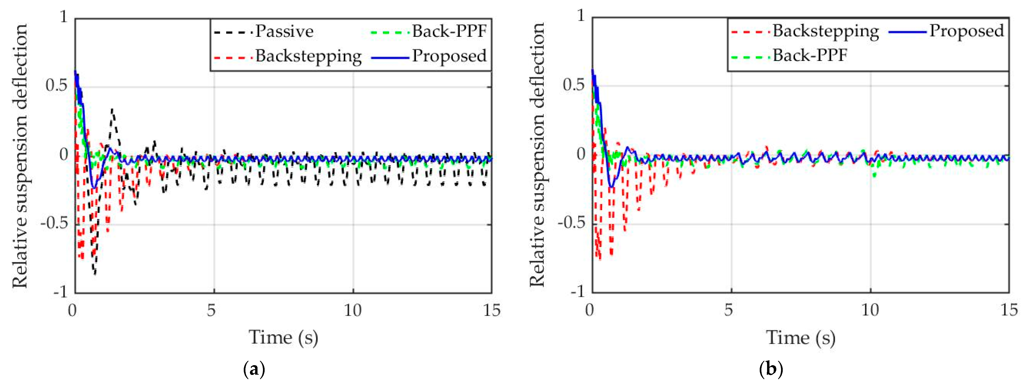
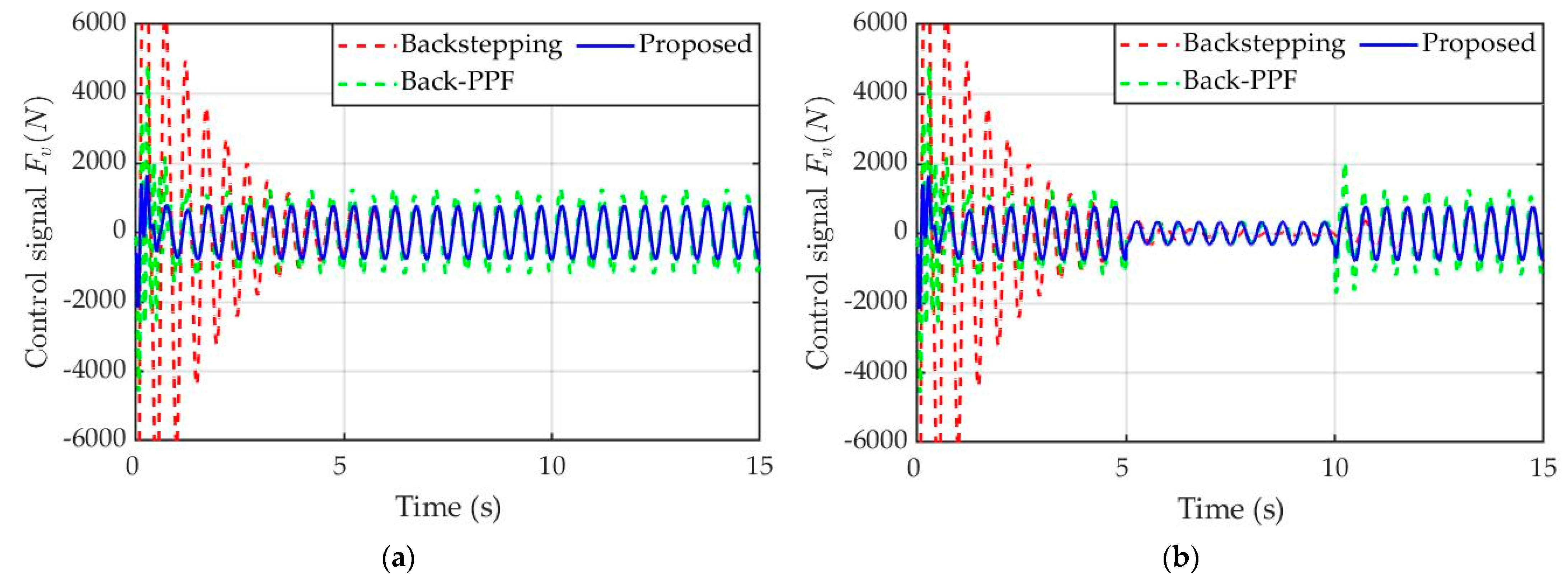
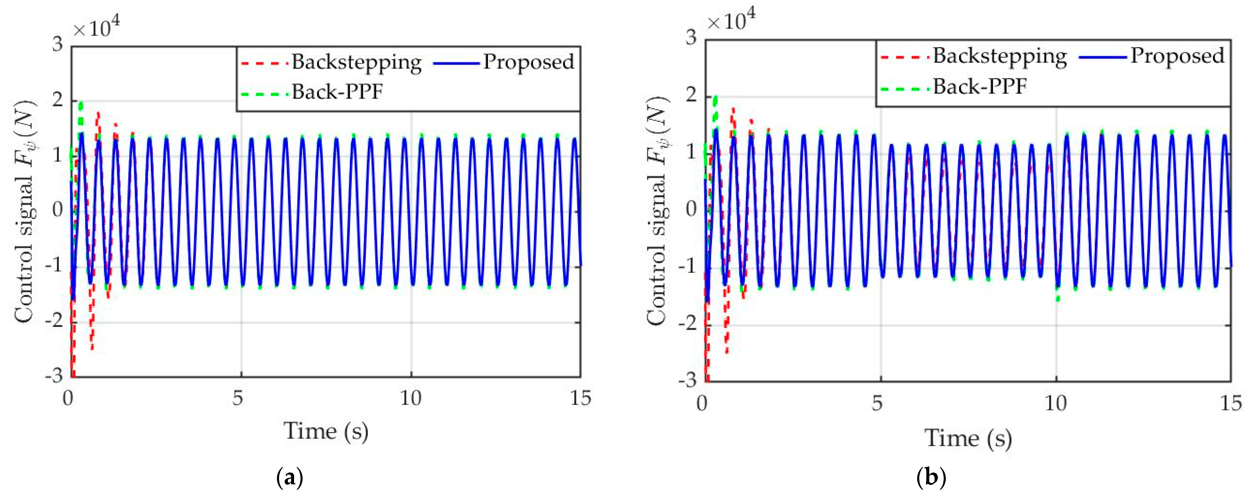
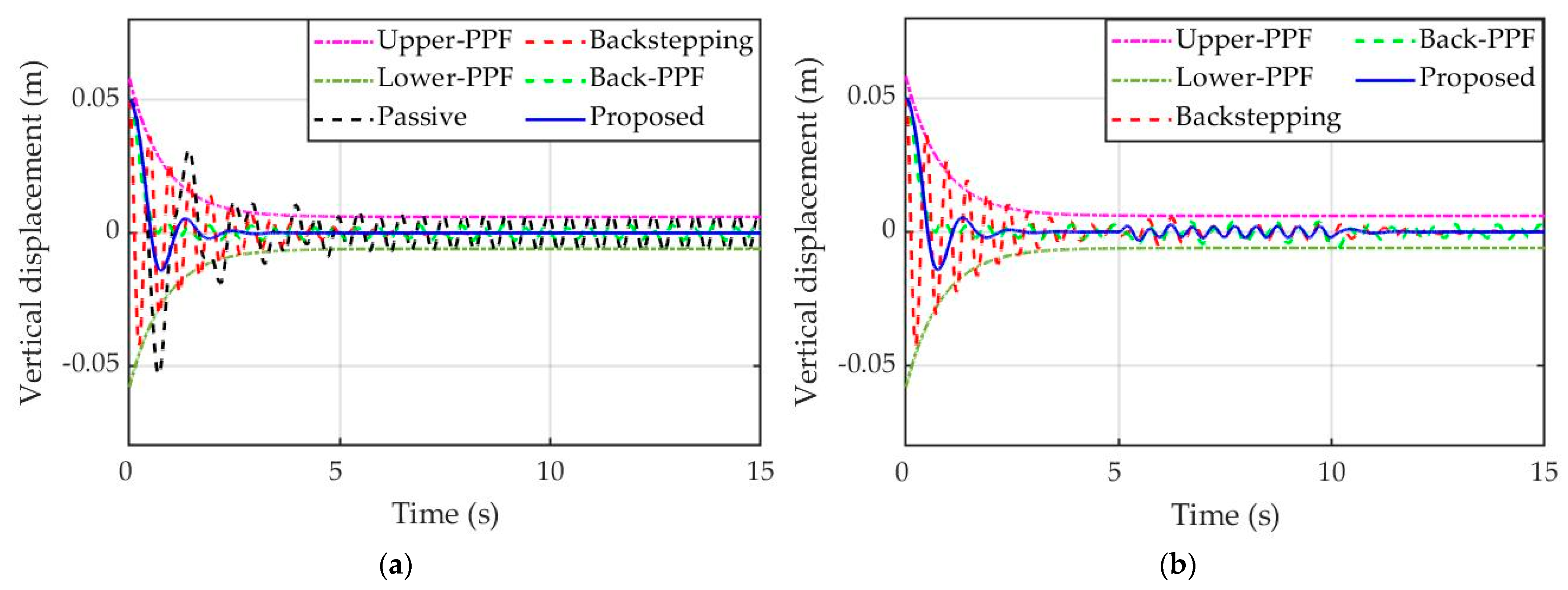
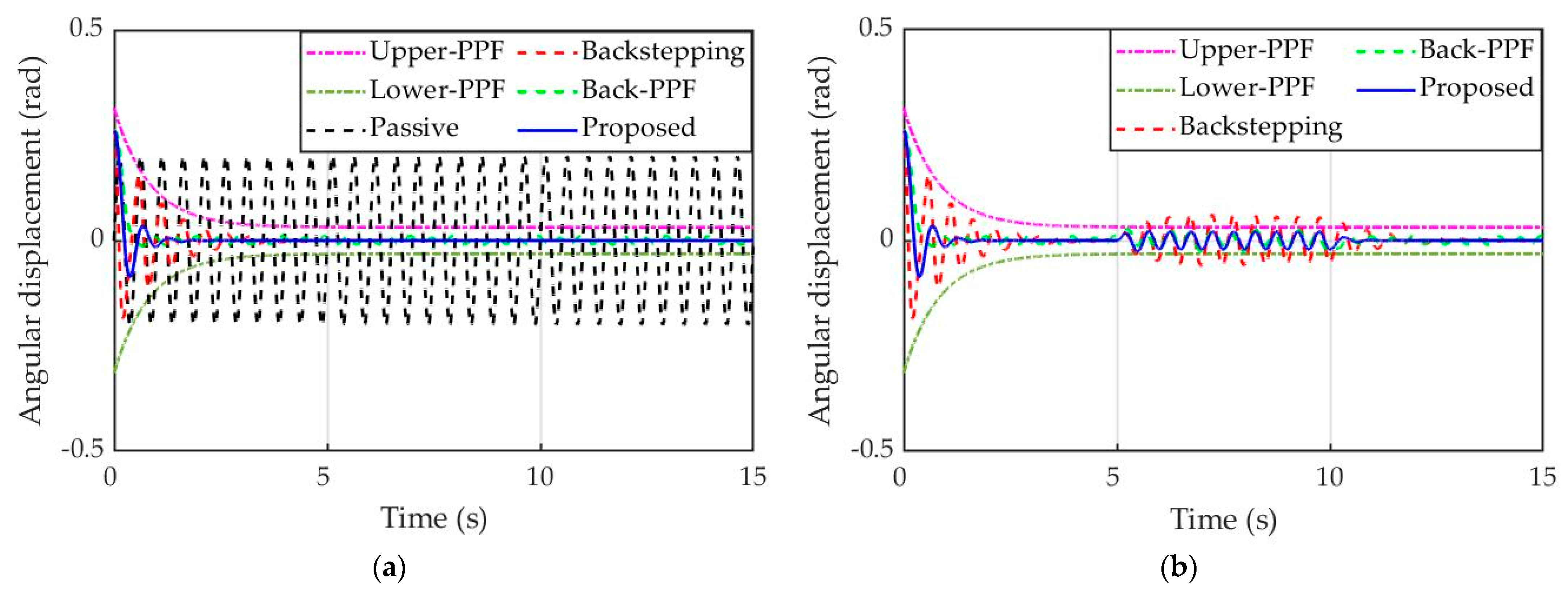
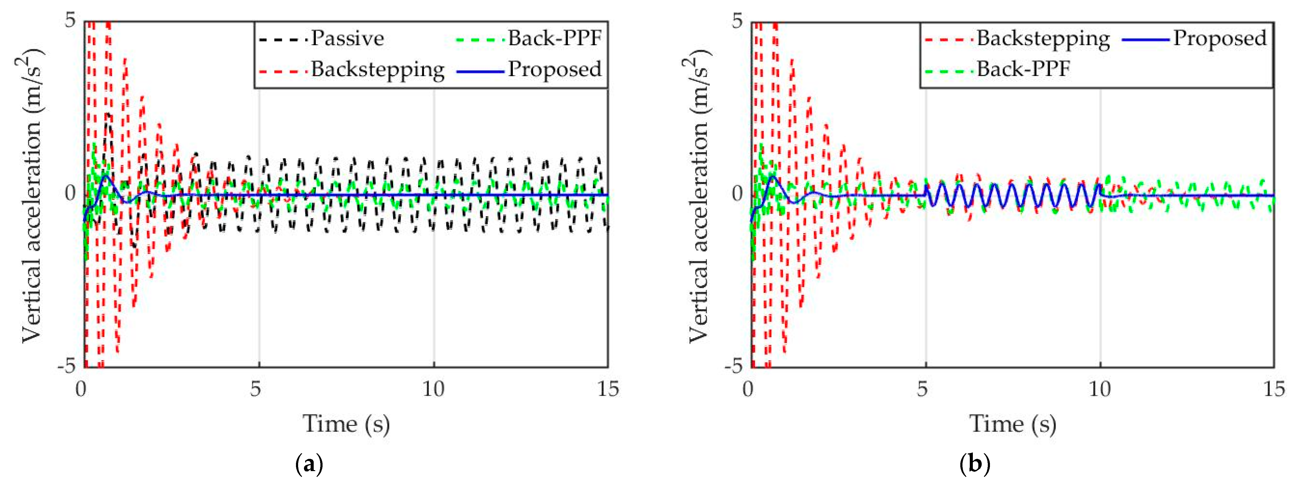
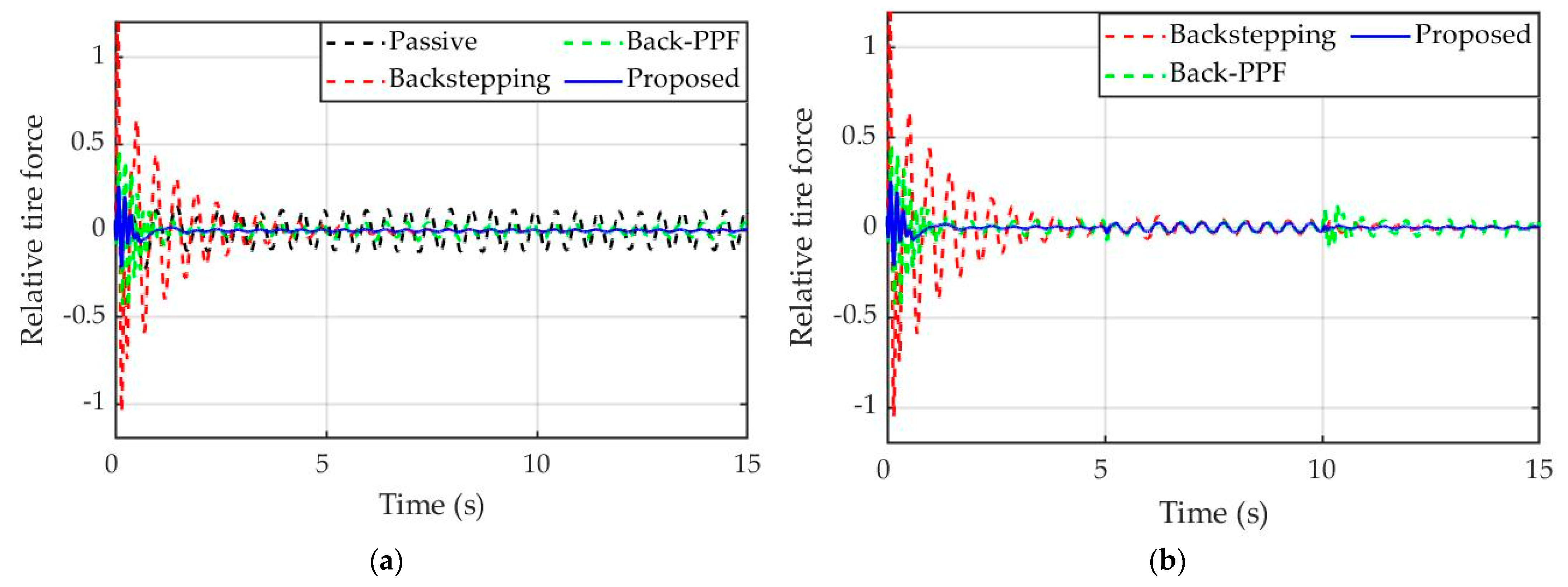
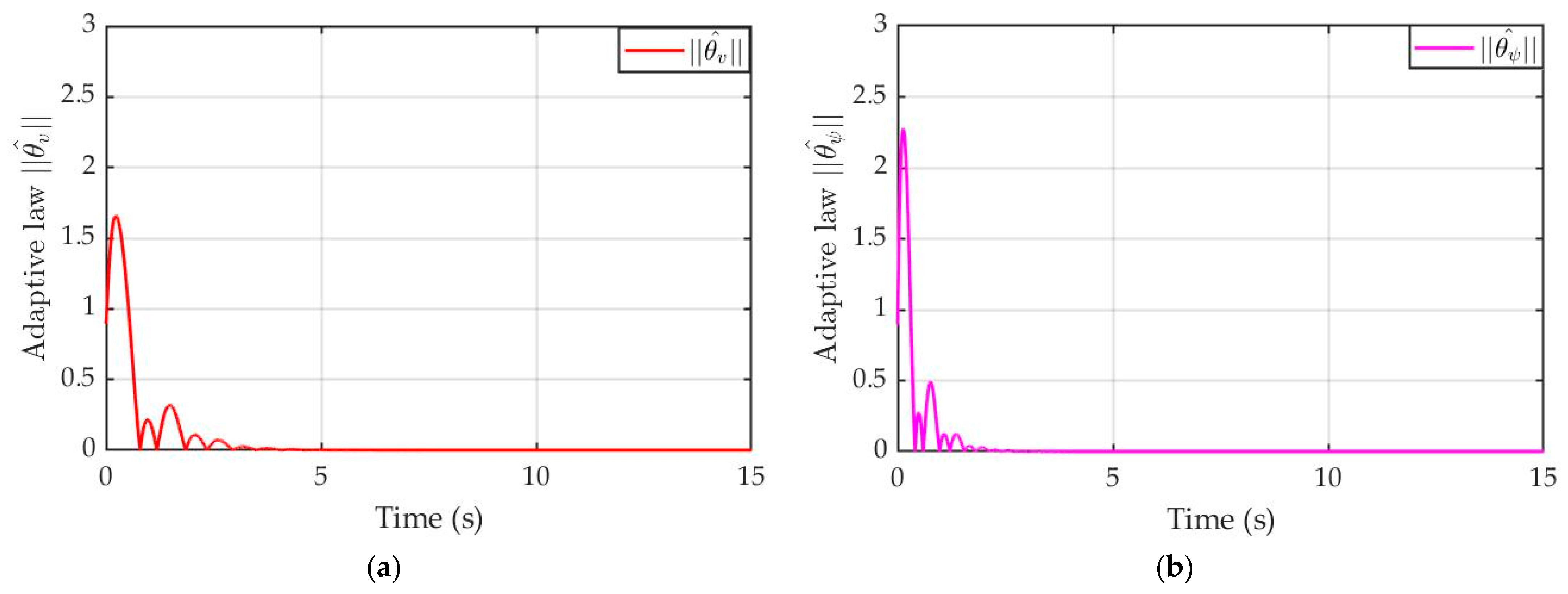
4. Simulation Results and Discussion

4.1. Simulation Description

This section provides comparative simulations to verify the effectiveness of the proposed control scheme in comparison with passive suspension, traditional backstepping, and backstepping with PPF (Back-PPF). To simulate the road disturbance, the sinusoidal profiles with an amplitude of 0.2 m and frequency of 2 Hz are used in this research by $z_{rf}(t)=0.2sin(4\pi t)$, $z_{rr}(t)=0.2sin(4\pi t+\pi )$. The simulation results of RSD and RTF objectives are also evaluated to prove suspension performance. The PPF constraints are chosen by ${\delta }_{01}=0.058,\hspace{0.17em}{\delta }_{\infty 1}=0.006,\hspace{0.17em}{\gamma }_1=1.2$, ${\delta }_{02}=\pi /10,\hspace{0.17em}{\delta }_{\infty 2}=\pi /100,\hspace{0.17em}{\gamma }_2=1.2$. The main parameters of the half-car suspension system can be displayed in

Table 1. Half-car suspension parameters.

Parameter	Value	Unit
$m_s$	1200	kg
$m_{uf}$	100	kg
$m_{ur}$	100	kg
$I$	600	kgm2
$k_{sf}$$,k_{sr}$	15,000	Nm−1
$k_{tf}$	150,000	Nm−1
$k_{tr}$	200,000	Nm−1
$c_{df}$$,c_{dr}$	1500	Nsm−1
$c_{tf}$	1100	Nsm−1
$c_{tr}$	1200	Nsm−1
$c$	1.2	m
$d$	1.5	m

.

Besides, the control parameters of different control methods are compared in

Table 2. Half-car suspension parameters.

Controller	Parameter
Backstepping	$k_1=40,\hspace{0.17em}{k}_2=60$
Back-PPF	$\begin{array}{l}{k}_1=40,\hspace{0.17em}{k}_2=60\\ {\overline{\beta }}_1=0.98;{\underset{\_}{\beta }}_1=0.98;\\ {\overline{\beta }}_2=0.98;{\underset{\_}{\beta }}_2=0.98;\end{array}$
Proposed	$\begin{array}{l}{k}_1=40,\hspace{0.17em}{k}_2=60\\ {\kappa }_1=5;{\varsigma }_v=0.1;{\rho }_v=10\\ {\kappa }_2=3;{\varsigma }_{\psi }=0.2;{\rho }_{\psi }=5\end{array}$

.

4.2. Simulation Results

The simulation results of vertical and angular motions of sprung mass and acceleration, RSD and RTF, are shown in Figure 3, Figure 4, Figure 5, Figure 6, Figure 7 and Figure 8. The tracking error of sprung mass displacement and angular motions are guaranteed within the small boundaries by the proposed control as displayed in Figure 3a and Figure 4a. With the PPF constraint, the proposed controller can provide a fast transient convergence speed than the other controllers. Under the effects of uncertain parameters, the passive cannot satisfy vehicle performance. Although the Back-PPF can limit both tracking errors of vertical and angular motions in comparison with the traditional backstepping, the sprung mass displacement cannot be stabilized to zero. The proposed control not only regulates the chassis movement within the small boundaries rapidly but also enhances the ride comfort even when the actuator failures occur at the time $5s<t<10s$. Because the traditional backstepping cannot compensate for the actuator faults, the chassis motions are more violated than the proposed scheme. Besides, the RMS acceleration value of the developed method is decreased by 68.1% to improve ride comfort in comparison with the Back-PPF as shown in Figure 5 and Figure 6. With the fault compensation technique, the vertical and angular accelerations of the proposed control can be reduced under the effects of actuator failures. The objectives of handling stability and driving safety are shown in Figure 7 and Figure 8. It can be seen that the suspension defection and dynamic tire load are guaranteed within the limitation ranges. The proposed control can decrease the RSD and RTF in comparison with the other methods to get the suspension objectives. To compare the control signals, the simulation results are displayed in Figure 9 and Figure 10; the developed control approach requires a smaller control signal in both fault and non-fault cases compared with other controllers. Furthermore, the convergence simulation results of the adaptive laws are shown in Figure 11.

5. Conclusions

This study proposed an adaptive fault tolerance control scheme for the half-car suspension system to stabilize both the vertical movement and angular displacement. The actuator failures are considered to investigate the suspension performance in the presence of uncertain parameters. FLSs are employed to approximate the unknown functions and are then incorporated into the control design to compensate for the effects of actuator faults. By applying the PPF technique, the proposed control not only eliminates the sprung mass displacement and angular motion to achieve the ride comfort but also guarantees the objectives of handling stability and driving safety. Then, the stability of the closed-loop system is analyzed according to the Lyapunov theorem. The RMS acceleration value is decreased by 68.1% when the proposed control is used for the simulation with the sin road profile. Hence, the developed control can provide an effective method for vehicle suspension, which can be applied to the automotive industry. Future research will focus on stabilizing the full car model with the PPF technique.

References

1. Rath, J.J.; Defoort, M.; Sentouh, C.; Karimi, H.R.; Veluvolu, K.C. Output-Constrained Robust Sliding Mode Based Nonlinear Active Suspension Control. IEEE Trans. Ind. Electron. 2020, 67, 10652–10662. [Google Scholar] [CrossRef]
2. Lin, B.; Su, X. Fault-tolerant Controller Design for Active Suspension System with Proportional Differential Sliding Mode Observer. Int. J. Control Autom. Syst. 2019, 17, 1751–1761. [Google Scholar] [CrossRef]
3. Liu, Y.-J.; Zeng, Q.; Liu, L.; Tong, S. An Adaptive Neural Network Controller for Active Suspension Systems with Hydraulic Actuator. IEEE Trans. Syst. Man Cybern. Syst. 2020, 50, 5351–5360. [Google Scholar] [CrossRef]
4. Pan, J.; Li, W.; Zhang, H. Control Algorithms of Magnetic Suspension Systems Based on the Improved Double Exponential Reaching Law of Sliding Mode Control. Int. J. Control Autom. Syst. 2018, 16, 2878–2887. [Google Scholar] [CrossRef]
5. Choi, H.D.; Lee, C.J.; Lim, M.T. Fuzzy Preview Control for Half-vehicle Electro-hydraulic Suspension System. Int. J. Control Autom. Syst. 2018, 16, 2489–2500. [Google Scholar] [CrossRef]
6. Jing, H.; Wang, R.; Li, C.; Bao, J. Robust finite-frequency H control of full-car active suspension. J. Sound Vib. 2019, 441, 221–239. [Google Scholar] [CrossRef]
7. Yan, G.; Fang, M.; Xu, J. Analysis and experiment of time-delayed optimal control for vehicle suspension system. J. Sound Vib. 2019, 446, 144–158. [Google Scholar] [CrossRef]
8. Pan, H.; Sun, W. Nonlinear Output Feedback Finite-Time Control for Vehicle Active Suspension Systems. IEEE Trans. Ind. Inform. 2019, 15, 2073–2082. [Google Scholar] [CrossRef]
9. Ho, C.M.; Tran, D.T.; Ahn, K.K. Adaptive sliding mode control based nonlinear disturbance observer for active suspension with pneumatic spring. J. Sound Vib. 2021, 509, 116241. [Google Scholar] [CrossRef]
10. Sun, W.; Gao, H.; Kaynak, O. Adaptive Backstepping Control for Active Suspension Systems with Hard Constraints. IEEE ASME Trans. Mechatron. 2013, 18, 1072–1079. [Google Scholar] [CrossRef]
11. Kazemipour, A.; Novinzadeh, A.B. Adaptive fault-tolerant control for active suspension systems based on the terminal sliding mode approach. Proc. Inst. Mech. Eng. Part C J. Mech. Eng. Sci. 2020, 234, 501–511. [Google Scholar] [CrossRef]
12. Pusadkar, U.S.; Chaudhari, S.D.; Shendge, P.D.; Phadke, S.B. Linear disturbance observer based sliding mode control for active suspension systems with non-ideal actuator. J. Sound Vib. 2019, 442, 428–444. [Google Scholar] [CrossRef]
13. Pang, H.; Zhang, X.; Chen, J.; Liu, K. Design of a coordinated adaptive backstepping tracking control for nonlinear uncertain active suspension system. Appl. Math. Model. 2019, 76, 479–494. [Google Scholar] [CrossRef]
14. Li, W.; Xie, Z.; Zhao, J.; Wong, P.K.; Li, P. Fuzzy finite-frequency output feedback control for nonlinear active suspension systems with time delay and output constraints. Mech. Syst. Signal Processing 2019, 132, 315–334. [Google Scholar] [CrossRef]
15. Ho, C.M.; Tran, D.T.; Nguyen, C.H.; Ahn, K.K. Adaptive Neural Command Filtered Control for Pneumatic Active Suspension with Prescribed Performance and Input Saturation. IEEE Access 2021, 9, 56855–56868. [Google Scholar] [CrossRef]
16. Zhang, Y.; Liu, Y.; Wang, Z.; Bai, R.; Liu, L. Neural networks-based adaptive dynamic surface control for vehicle active suspension systems with time-varying displacement constraints. Neurocomputing 2020, 408, 176–187. [Google Scholar] [CrossRef]
17. Li, H.; Zhang, Z.; Yan, H.; Xie, X. Adaptive Event-Triggered Fuzzy Control for Uncertain Active Suspension Systems. IEEE Trans. Cybern. 2019, 49, 4388–4397. [Google Scholar] [CrossRef]
18. Wen, S.; Chen, M.Z.Q.; Zeng, Z.; Yu, X.; Huang, T. Fuzzy Control for Uncertain Vehicle Active Suspension Systems via Dynamic Sliding-Mode Approach. IEEE Trans. Syst. Man Cybern. Syst. 2017, 47, 24–32. [Google Scholar] [CrossRef]
19. Bechlioulis, C.P.; Rovithakis, G.A. Robust Adaptive Control of Feedback Linearizable MIMO Nonlinear Systems with Prescribed Performance. IEEE Trans. Autom. Control 2008, 53, 2090–2099. [Google Scholar] [CrossRef]
20. Yang, Y.; Tan, J.; Yue, D. Prescribed performance control of one-DOF link manipulator with uncertainties and input saturation constraint. IEEE CAA J. Autom. Sin. 2019, 6, 148–157. [Google Scholar] [CrossRef]
21. Wang, M.; Yang, A. Dynamic Learning from Adaptive Neural Control of Robot Manipulators with Prescribed Performance. IEEE Trans. Syst. Man Cybern. Syst. 2017, 47, 2244–2255. [Google Scholar] [CrossRef]
22. Huang, Y.; Na, J.; Wu, X.; Gao, G. Approximation-Free Control for Vehicle Active Suspensions with Hydraulic Actuator. IEEE Trans. Ind. Electron. 2018, 65, 7258–7267. [Google Scholar] [CrossRef]
23. Na, J.; Huang, Y.; Wu, X.; Gao, G.; Herrmann, G.; Jiang, J.Z. Active Adaptive Estimation and Control for Vehicle Suspensions with Prescribed Performance. IEEE Trans. Control Syst. Technol. 2018, 26, 2063–2077. [Google Scholar] [CrossRef] [Green Version]
24. Liu, S.; Jiang, B.; Mao, Z.; Ding, S.X. Adaptive Backstepping Based Fault-tolerant Control for High-speed Trains with Actuator Faults. Int. J. Control Autom. Syst. 2019, 17, 1408–1420. [Google Scholar] [CrossRef]
25. Pan, H.; Li, H.; Sun, W.; Wang, Z. Adaptive Fault-Tolerant Compensation Control and Its Application to Nonlinear Suspension Systems. IEEE Trans. Syst. Man Cybern. Syst. 2020, 50, 1766–1776. [Google Scholar] [CrossRef]
26. Chen, L.; Li, X.; Xiao, W.; Li, P.; Zhou, Q. Fault-tolerant Control for Uncertain Vehicle Active Steering Systems with Time-delay and Actuator Fault. Int. J. Control Autom. Syst. 2019, 17, 2234–2241. [Google Scholar] [CrossRef]
27. Ho, C.M.; Ahn, K.K. Design of an Adaptive Fuzzy Observer-Based Fault Tolerant Controller for Pneumatic Active Suspension with Displacement Constraint. IEEE Access 2021, 9, 136346–136359. [Google Scholar] [CrossRef]
28. Liu, B.; Saif, M.; Fan, H. Adaptive Fault Tolerant Control of a Half-Car Active Suspension Systems Subject to Random Actuator Failures. IEEE ASME Trans. Mechatron. 2016, 21, 2847–2857. [Google Scholar] [CrossRef]
29. Liu, S.; Zhou, H.; Luo, X.; Xiao, J. Adaptive sliding fault tolerant control for nonlinear uncertain active suspension systems. J. Frankl. Inst. 2016, 353, 180–199. [Google Scholar] [CrossRef]
30. Wang, L.-X.; Mendel, J.M. Fuzzy basis functions, universal approximation, and orthogonal least squares learning. IEEE Trans. Neural Netw. 1992, 3, 807–814. [Google Scholar] [CrossRef] [Green Version]
31. Wang, L.-X. Stable adaptive fuzzy control of nonlinear systems. IEEE Trans. Fuzzy Syst. 1993, 1, 146–155. [Google Scholar] [CrossRef]
32. Liu, H.; Li, X.; Liu, X.; Wang, H. Adaptive Neural Network Prescribed Performance Bounded- Hinfinity Tracking Control for a Class of Stochastic Nonlinear Systems. IEEE Trans. Neural. Netw. Learn. Syst. 2020, 31, 2140–2152. [Google Scholar] [CrossRef] [PubMed]
Figure 1. Half car active suspension model.
Electronics 11 01733 g001
Figure 2. Fuzzy membership functions.
Electronics 11 01733 g002
Figure 3. Sprung mass vertical displacement: (a) Non-fault; (b) Actuator-fault.
Electronics 11 01733 g003
Figure 4. Sprung mass angular displacement: (a) Non-fault; (b) Actuator-fault.
Electronics 11 01733 g004
Figure 5. Sprung mass vertical acceleration: (a) Non-fault; (b) Actuator-fault.
Electronics 11 01733 g005
Figure 6. Sprung mass angular acceleration: (a) Non-fault; (b) Actuator-fault.
Electronics 11 01733 g006
Figure 7. Relative suspension deflection responses: (a) Non-fault; (b) Actuator-fault.
Electronics 11 01733 g007
Figure 8. Relative tire force responses: (a) Non-fault; (b) Actuator-fault.
Electronics 11 01733 g008
Figure 9. Control signals F v (N): (a) Non-fault; (b) Actuator-fault.
Electronics 11 01733 g009
Figure 10. Control signals F ψ (N): (a) Non-fault; (b) Actuator-fault.
Electronics 11 01733 g010
Figure 11. Adaptive law: (a) θ ^ v ; (b) θ ^ ψ .
Electronics 11 01733 g011