Study on the Compact Balance Control Mechanism for Guinea Fowl Jumping Robot

Abstract

We developed a guinea fowl jumping robot with a one-axis momentum wheel mechanism with a passive hallux model. The Guinea fowl jumping robot was able to perform stable vertical jumping due to the linkage structure designed as a passive hallux model. Furthermore, we used the one-axis momentum wheel mechanism in the jumping robot for making the compact balance control mechanism that can control the body angle of the robot. Through the experiment, the conventional jumping robot uses the inertial tail to adjust the body angle in the air for stable landing and jumping. However, in the case of an inertial tail, it has a large volume and has a disadvantage in that stability is highly reduced when it collides with obstacles due to the shape of the inertial tail. Moreover, we performed a theoretical analysis, simulation, and experiment to verify the performance of the momentum wheel mechanism, and we confirmed that the passive hallux structure contributed to the jumping stability. Besides, we proved that the momentum wheel could adequately land on the ground by adjusting the body angle after vertical jumping. In addition, we demonstrated that the stability of the momentum wheel is higher than the inertial tail through collision simulation.

1. Introduction

Jumping robots can quickly overcome obstacles of varying height. Due to such advantages, the jumping robot can be used in various environments that have rough terrain [1,2,3]. To overcome the rough terrain using a jumping robot, a linkage design of the leg model and a balance control mechanism need to be considered [1,2,3,4,5]. When applying a linkage model to the jumping robot, the robot can move all links of the leg model by using only a single motor, and this can reduce the jumping robot’s control elements, volume, and weight. For these reasons, the control efficiency of the linkage model is higher than that of a multi-node model. Recently, many researchers have mimicked an animal leg structure to design the jumping robot’s legs using a linkage structure [1,2,3,4,5,6,7]. Besides, to control the posture of the jumping robot, a balance control mechanism has been actively studied.

In the case of [8,9], these robots use 1-DOF to operate the whole linkage model. However, these robots cannot control the jumping height, tilting angle, and the distance of jumping forward because the trajectory of leg structure is fixed. As a result, to control the jumping angle, jump height, and distance of jumping forward, these robots need a balance control mechanism. Refs. [8,9] rotate the inertial tail after jumping to stand the fallen jumping robot on the ground by controlling the posture. However, with this method, it is difficult to control the jumping angle and the jumping height in real-time and continuous jumping cannot be performed.

In addition, researchers also studied the control method for the inertial tail by using a 2-DOF servo [10] or pneumatic actuator [11]. However, these two studies are not suitable as a balance control mechanism for a small jumping robot because several servos are used to move the inertial tail and a pneumatic mechanism that occupies a large volume is applied.

For continuous jumping in real-time without falling, it is necessary to control the body angle of the jumping robot during the stance phase or takeoff phase. In the case of the Penn Jerboa robot [12] and Salto-1P [13], the inertial tail mechanism can control the body angle of the robot in the air, and these robots can change the jumping height and tilting angle by controlling the posture of the robot during the stance phase or takeoff phase. This control technique allows the jumping robot to perform agile continuous jumping. Interestingly, when these robots start initial jumping, they perform the vertical jumping, because the jumping robot can reach the maximum height rapidly, and can earn enough time to control the body angle before landing. Moreover, the inertial tail mechanism can support a large control output. However, the inertial tail has a disadvantage in that it occupies a huge volume and has a high probability of colliding with obstacles. As a result, it is necessary to make a compact balance control mechanism that has similar control performance. In addition, to increase the stability of agile jumping, the jumping robot needs a leg model that makes it possible for the feet to be parallel with the ground and maintain balance when the legs move rapidly.

To solve the problem of the inertial tail mechanism, a study on the guinea fowl jumping robot using a momentum wheel was also undertaken [14,15]. However, in a study on vertical jumping using the guinea fowls leg model, the hallux model for vertical jumping stably was not considered. Furthermore, it was not verified whether the momentum wheel could achieve stable control performance while having a compact design compared to the inertial tail.

The structure of this paper, aiming to compare the stability of the aforementioned robot legs and the stability of the momentum wheel and inertial tail, is as follows. In Section 2, the linkage design for the passive hallux model that assists the guinea fowl jumping robot to jump stably when performing vertical jumping will be mentioned, and a dynamic model for the jumping robot and momentum wheel will be created and analyzed through equations. Furthermore, we will cover the design of the jumping robot based on the analysis. In Section 3, we will verify the jumping performance and the performance of the momentum wheel based on the designed robot and perform collision simulation to compare the stability of the momentum wheel and the inertial tail.

2. Design of Guinea Fowl Jumping Robot with Momentum Wheel

This section will cover the design of the guinea fowl jumping robot and the momentum wheel mechanism. Then, we will analyze the dynamic model of the guinea fowl jumping robot and the momentum wheel model.

2.1. Design of Leg Model of Guinea Fowl Jumping Robot

The vertical jumping performance of the guinea fowl is important to control the jumping angle of the robot in the air. To provide vertical jumping, we consider the limb angle and bone structure. First, to design the linkage structure, it is necessary to see how the leg angle of the guinea fowl changes over time. As described in [16], the preparation time for jumping required is 270 ms from the initial position and the jumping energy value reaches the maximum at 0 ms. The state when the guinea fowl has maximum jumping energy is called the pre-takeoff (PRT) stage. The guinea fowl starts to release the jumping energy using the leg muscles at 0 ms, and the time of maximum jumping energy emission is 120 ms. At 120 ms, the guinea fowl fully stretches its two legs, and this state is called the post-takeoff (POT) stage.

To construct the linkage model based on the limbs of the guinea fowl, it is necessary to analyze how the leg angle changes when the state changes from PRT to POT. This reference also investigated the limb angle of the guinea fowl model: in the initial motion of the guinea fowl, hip angle, knees angle, ankle angle, and toe angle are 43 $\pm$ 5 degrees, 64 $\pm$ 3 degrees, and 90 $\pm$ 9 degrees, respectively. When the guinea fowl moves its posture into PRT, hip angle, knees angle, ankle angle, and toe angle become 30 $\pm$ 3 degrees, 54 $\pm$ 4 degrees, 45 $\pm$ 5 degrees, and 160 $\pm$ 3 degrees, respectively. Finally, at the POT stage, hip angle, knees angle, ankle angle, and toe angle are 98 $\pm$ 3 degrees, 97 $\pm$ 4 degrees, 154 $\pm$ 5 degrees, and 173 $\pm$ 4 degrees, respectively, and the guinea fowl fully stretches the limb and starts to take-off.

Besides, we consider the bone structure of the guinea fowl’s leg. The leg consists of the femur, tibiotarsus, tarsometatarsal, digits, and hallux. We measured the bone length introduced in the reference so we could determine that the length ratio of the limb bone is 1:1.5:0.8:0.75:0.37 [16,17,18,19].

The linkage model of the robot is created by mimicking the joint angle and the bone structure of the guinea fowl model shown in Figure 1. This linkage structure is designed such that the whole link can move using one motor and it is considered the bone length ratio of the guinea fowl model. In the actual guinea fowl bone model, the tarsometatarsal and the digits are composed of different bones. However, in the designed linkage model, these two parts are united. This is because the designed robot’s legs can only be moved by one motor.

The guinea fowl moves digits when jumping or running, allowing it to move more efficiently depending on the environment. To create this motion, we need an additional motor, but if we attach an additional motor, the jumping robot becomes heavy. To solve these problems, we designed the hallux that can move passively when the digits angle is changed. In Figure 1, when the guinea fowl robot changes from the PRT (left) to the POT (right), the legs can stably stand on the ground. We used the LINKAGE program to test the designed linkage model. The simulation results are shown in Figure 2c. We confirmed that the hallux can stably contact the ground, and we checked that the trajectory of jumping is vertical.

Then, we carried out a closed loop equation and simulation to assess whether the non-passive hallux model can perform the PRT and POT stages on the ground. Figure 2a shows the closed-loop equation model for the jumping trajectory that changes when the non-passive hallux model is moved from POT to PRT. Figure 2a shows the trajectory of the joint of hallux (${\mathrm{T}}_{\mathrm{j}}$) that changes when the rotational joint ($\mathrm{D}$) rotates by ${\mathsf{\psi }}_{\mathrm{j}}$. In the linkage model, each joint point is defined from A to $\mathrm{T}$, and the coordinates of each point are defined as $\overrightarrow{\mathrm{A}}={\mathrm{A}}_{\mathrm{x}}+{\mathrm{A}}_{\mathrm{y}}\mathrm{i}$. Next, the rotation angle for each link is expressed in the form of ${\mathrm{e}}^{\mathrm{i}\mathsf{\psi }}$. In Figure 2a, the closed-loop equation for the ground joints A, B, C, and D to the joint of hallux (${\mathrm{T}}_{\mathrm{j}}$) can be defined by Equations (1)–(7). Through Equations (6) and (7), we can obtain the ${\mathrm{T}}_{\mathrm{j}}$ coordinates that change according to the rotation angle of the motor, and the optimal values for the length and change angle of each link can be obtained using Equations (1)–(7).

$$\begin{gathered} \overrightarrow{\mathrm{A}}+{\mathrm{e}}^{\mathrm{i}{\mathsf{\varphi }}_{\mathrm{j}}}\left(\overrightarrow{\mathrm{I}}-\overrightarrow{\mathrm{A}}\right)=\overrightarrow{\mathrm{B}}+{\mathrm{e}}^{{\mathrm{i}\mathsf{\omega }}_{\mathrm{j}}}\left(\overrightarrow{\mathrm{H}}-\overrightarrow{\mathrm{B}}\right)+{\mathrm{e}}^{{\mathrm{i}\mathsf{\rho }}_{\mathrm{j}}}\left(\overrightarrow{\mathrm{I}}-\overrightarrow{\mathrm{H}}\right)=\overrightarrow{\mathrm{C}}+{\mathrm{e}}^{{\mathrm{i}\mathsf{\lambda }}_{\mathrm{j}}}\left(\overrightarrow{\mathrm{G}}-\overrightarrow{\mathrm{C}}\right)+ \\ {\mathrm{e}}^{{\mathrm{i}\mathsf{\epsilon }}_{\mathrm{j}}}\left(\overrightarrow{\mathrm{H}}-\overrightarrow{\mathrm{G}}\right)+{\mathrm{e}}^{{\mathrm{i}\mathsf{\rho }}_{\mathrm{j}}}\left(\overrightarrow{\mathrm{I}}-\overrightarrow{\mathrm{H}}\right), \end{gathered}$$

(1)

$$\begin{array}{ll}\overrightarrow{\mathrm{A}}+{\mathrm{e}}^{\mathrm{i}{\mathsf{\varphi }}_{\mathrm{j}}}\left(\overrightarrow{\mathrm{I}}-\overrightarrow{\mathrm{A}}\right)& =\overrightarrow{\mathrm{D}}+{\mathrm{e}}^{{\mathrm{i}\mathsf{\psi }}_{\mathrm{j}}}\left(\overrightarrow{\mathrm{E}}-\overrightarrow{\mathrm{D}}\right)+{\mathrm{e}}^{{\mathrm{i}\mathsf{\mu }}_{\mathrm{j}}}\left(\overrightarrow{\mathrm{F}}-\overrightarrow{\mathrm{E}}\right)+{\mathrm{e}}^{{\mathrm{i}\mathsf{\lambda }}_{\mathrm{j}}}\left(\overrightarrow{\mathrm{G}}-\overrightarrow{\mathrm{F}}\right)+{\mathrm{e}}^{{\mathrm{i}\mathsf{\epsilon }}_{\mathrm{j}}}\left(\overrightarrow{\mathrm{H}}-\overrightarrow{\mathrm{G}}\right)\\ & +{\mathrm{e}}^{{\mathrm{i}\mathsf{\rho }}_{\mathrm{j}}}\left(\overrightarrow{\mathrm{I}}-\overrightarrow{\mathrm{H}}\right),\end{array}$$

(2)

$$\overrightarrow{\mathrm{B}}+{\mathrm{e}}^{{\mathrm{i}\mathsf{\omega }}_{\mathrm{j}}}\left(\overrightarrow{\mathrm{H}}-\overrightarrow{\mathrm{B}}\right)=\overrightarrow{\mathrm{C}}+{\mathrm{e}}^{{\mathrm{i}\mathsf{\lambda }}_{\mathrm{j}}}\left(\overrightarrow{\mathrm{G}}-\overrightarrow{\mathrm{C}}\right)+{\mathrm{e}}^{{\mathrm{i}\mathsf{\epsilon }}_{\mathrm{j}}}\left(\overrightarrow{\mathrm{H}}-\overrightarrow{\mathrm{G}}\right),$$

(3)

$$\overrightarrow{\mathrm{C}}+{\mathrm{e}}^{{\mathrm{i}\mathsf{\lambda }}_{\mathrm{j}}}\left(\overrightarrow{\mathrm{G}}-\overrightarrow{\mathrm{C}}\right)=\overrightarrow{\mathrm{D}}+{\mathrm{e}}^{{\mathrm{i}\mathsf{\psi }}_{\mathrm{j}}}\left(\overrightarrow{\mathrm{E}}-\overrightarrow{\mathrm{D}}\right)+{\mathrm{e}}^{{\mathrm{i}\mathsf{\mu }}_{\mathrm{j}}}\left(\overrightarrow{\mathrm{F}}-\overrightarrow{\mathrm{E}}\right)+{\mathrm{e}}^{{\mathrm{i}\mathsf{\lambda }}_{\mathrm{j}}}\left(\overrightarrow{\mathrm{G}}-\overrightarrow{\mathrm{F}}\right),$$

(4)

$$\overrightarrow{\mathrm{B}}+{\mathrm{e}}^{{\mathrm{i}\mathsf{\omega }}_{\mathrm{j}}}(\overrightarrow{\mathrm{H}}-\overrightarrow{\mathrm{B}})+{\mathrm{e}}^{{\mathrm{i}\mathsf{\epsilon }}_{\mathrm{j}}}\left(\overrightarrow{\mathrm{G}}-\overrightarrow{\mathrm{H}}\right)=\overrightarrow{\mathrm{D}}+{\mathrm{e}}^{{\mathrm{i}\mathsf{\psi }}_{\mathrm{j}}}\left(\overrightarrow{\mathrm{E}}-\overrightarrow{\mathrm{D}}\right)+{\mathrm{e}}^{{\mathrm{i}\mathsf{\mu }}_{\mathrm{j}}}\left(\overrightarrow{\mathrm{F}}-\overrightarrow{\mathrm{E}}\right)+{\mathrm{e}}^{{\mathrm{i}\mathsf{\lambda }}_{\mathrm{j}}}\left(\overrightarrow{\mathrm{G}}-\overrightarrow{\mathrm{F}}\right),$$

(5)

$$\overrightarrow{\mathrm{A}}+{\mathrm{e}}^{\mathrm{i}{\mathsf{\varphi }}_{\mathrm{j}}}\left(\overrightarrow{\mathrm{I}}-\overrightarrow{\mathrm{A}}\right)+{\mathrm{e}}^{{\mathrm{i}\mathsf{\rho }}_{\mathrm{j}}}\left(\overrightarrow{\mathrm{K}}-\overrightarrow{\mathrm{I}}\right)+{\mathrm{e}}^{{\mathrm{i}\mathsf{\xi }}_{\mathrm{j}}}\left(\overrightarrow{{\mathrm{T}}_0}-\overrightarrow{\mathrm{K}}\right)=\overrightarrow{{\mathrm{T}}_{\mathrm{j}}},$$

(6)

$$\overrightarrow{\mathrm{B}}+{\mathrm{e}}^{{\mathrm{i}\mathsf{\omega }}_{\mathrm{j}}}\left(\overrightarrow{\mathrm{H}}-\overrightarrow{\mathrm{B}}\right)+{\mathrm{e}}^{{\mathrm{i}\mathsf{\rho }}_{\mathrm{j}}}\left(\overrightarrow{\mathrm{K}}-\overrightarrow{\mathrm{H}}\right)+{\mathrm{e}}^{{\mathrm{i}\mathsf{\xi }}_{\mathrm{j}}}\left(\overrightarrow{{\mathrm{T}}_0}-\overrightarrow{\mathrm{K}}\right)=\overrightarrow{{\mathrm{T}}_{\mathrm{j}}},$$

(7)

Then, we verified how the coordinate of the joint of the hallux rotates as the linkage structure changes, as shown in Figure 2b. In the non-passive hallux model, the angle between hallux and digit is fixed. When the initial coordinates of the joint of the hallux in the non-passive hallux model are set to ${\mathrm{T}}_0$(x,y), the coordinates of the joint of hallux that change from POT to PRT become ${\mathrm{T}}_{\mathrm{j}}$(x’,y’). In addition, before the non-passive hallux model moves, the point of contact with the ground is set to O(0,0), and point O is assumed as the anchor. Besides, the changing angle as the joint of hallux is defined as ${\mathsf{\Delta }\mathsf{\theta }}_{\mathrm{h}}$. As a result, we can define the vector equation as Equation (8). To increase the jumping stability when the robot changes from the POT stage to the PRT stage, ${\mathsf{\Delta }\mathsf{\theta }}_{\mathrm{h}}$ should be maintained at 0 degrees.

$$\left[\begin{array}{c}{\mathrm{x}}^{\prime }\\ {\mathrm{y}}^{\prime }\end{array}\right]=\left[\begin{array}{cc}{\cos \mathsf{\Delta }\mathsf{\theta }}_{\mathrm{h}}& -{\sin \mathsf{\Delta }\mathsf{\theta }}_{\mathrm{h}}\\ {\sin \mathsf{\Delta }\mathsf{\theta }}_{\mathrm{h}}& {\cos \mathsf{\Delta }\mathsf{\theta }}_{\mathrm{h}}\end{array}\right]\left[\begin{array}{c}\mathrm{x}\\ \mathrm{y}\end{array}\right],$$

(8)

The simulation results for the passive hallux model and the non-passive hallux model are shown in Figure 2c. The red line is the non-passive hallux model, and the blue line is the passive hallux model. Furthermore, it takes 120 ms for the robot to change the motion from the POT stage to the PRT stage. In the case of the non-passive hallux model, ${\mathsf{\Delta }\mathsf{\theta }}_{\mathrm{h}}$ changed from 0 degrees to 25 degrees over time. For this reason, when the robot reaches the PRT stage, the robot is lifted backwards and then tilted forwards from 120 ms to 240 ms. In contrast, the passive hallux model maintains the ${\mathsf{\Delta }\mathsf{\theta }}_{\mathrm{h}}$ to 0 degrees until the PRT stage, and hence the robot can stand stably when the robot reaches the POT to PRT stage.

In the case of Salto-1P, a non-passive hallux model can be used to initiate a jump only at the PRT stage. However, in the case of the passive hallux model, the jumping robot can start the first jump in the POT stage as well as the PRT stage. This advantage can increase the initial stability by positioning the robot such that it can return to its original position even if an initial jumping error occurs. As a result, the passive hallux model contributes to the stability of the pre-jumping motion and vertical jumping motion.

2.2. Design of Trigger Mechanism

To design the trigger mechanism, we considered a torsion spring and rubber band. The spring model corresponding to the muscle attached to the femur uses a torsion spring, and a rubber band is used to transmit the force between the femur and the tarsometatarsal. First, we chose the torsion springs model. We use four torsion springs to accumulate the jumping energy, and the spring constant is 38.3 Nmm/deg. Second, we consider the torsion spring part of the trigger mechanism. The implemented force transmission structure using the torsion spring model is shown in Figure 3a. The yellow part is the femur, and the torsion spring is fixed to the femur. The operation mechanism is as follows. First, when the motor moves, the cam pushes the roller and swinging bar to compress the torsion spring. When the torsion spring is fully compressed, the cam reaches the critical point. If the cam passes the critical point, the torsion spring starts to release the elastic energy.

Then, we considered the muscle located between the femur and the tarsometatarsal. For transmitting the jumping energy to the linkage model efficiently, we considered the leg model by mimicking the muscles of each part. The mechanism designed with a rubber band is shown in Figure 3b. As shown in Figure 3b, we attached the rubber band to the joint of the femur and the joint of the tarsometatarsal. As a result, when the whole link moves, the rubber band is stretched, and the jumping energy is accumulated. Like the torsion spring mechanism, when the cam passes the critical point, the elastic energy starts to release. We wound the rubber bands nine times to the limb model. In addition, we performed ten iterations of tensile tests and confirmed that the spring constant of the rubber band is 50 N/m.

After we chose the spring model and trigger mechanism, we calculated the jumping height. Our goal is to create a robot that can jump 20 cm without a balance control circuit. The equation for calculating the jumping height is given in Equation (9), where $\mathrm{h}$ is the jumping height, $\mathsf{\gamma }$ is the takeoff angle, and ${\mathrm{k}}_1$ is the stiffness coefficient of the torsion spring. $\mathsf{\theta }$ is the maximum compression angle of the torsion spring, ${\mathrm{N}}_1$ is the number of torsion springs, and ${\mathrm{N}}_2$ is the number of times the rubber band is wound. ${\mathrm{k}}_2$ is the stiffness coefficient of the rubber band, $\Delta \mathrm{x}$ is the stretched length of the rubber band, $\mathrm{I}$ is the moment of inertia of the jumping robot, $\mathsf{\omega }$ is the angular velocity that occurs when the robot starts jumping, and $\mathrm{m}$ is the mass of the guinea fowl jumping robot.

Table 1. The parameter values of the guinea fowl jumping robot.

Symbol	Parameter Value
${\mathrm{N}}_1$	4
${\mathrm{k}}_1$	38.3 Nmm/deg
$\mathsf{\theta }$	$17.73°$
$\mathsf{\gamma }$	$90°$
${\mathrm{N}}_2$	36
${\mathrm{k}}_2$	50 N/m
$\Delta \mathrm{x}$	3.8 cm
m	713 g
$\Delta \mathsf{\psi }$	$60°$
${\mathrm{P}}_1$	48.6 mm
${\mathrm{P}}_2$	3.0 mm
${\mathrm{N}}_1$	4
${\mathrm{k}}_1$	38.3 Nmm/deg
$\mathsf{\theta }$	$17.73°$

shows the parameter values for calculating the jumping height. Through the calculation, we confirmed that the jumping height is 25.3 cm and that the jumping robot can jump 20 cm.

$$\mathrm{h}=\left({\mathrm{N}}_1{\mathrm{k}}_1{\mathsf{\theta }}^2{\sin }^2\mathsf{\gamma }+{\mathrm{N}}_2{\mathrm{k}}_2{\mathrm{x}}^2-{\mathrm{I}\mathsf{\omega }}^2\right)/2\mathrm{mg},$$

(9)

To accumulate elastic energy using torsion springs and rubber bands, we selected a motor that can provide sufficient torque to the cam. The equation for obtaining the required torque to rotate the cam is given in Equation (10). ${\mathsf{\tau }}_{\mathrm{r}}$ is the required torque of the system, ${\mathrm{P}}_1$ is the distance between the point ${\mathrm{O}}^{\prime }$ and the operating line of force $\mathrm{F}$, ${\mathrm{P}}_2$ is the distance between the point $\mathrm{O}$ and the operating line of force $\mathrm{F}$, and $\Delta \mathsf{\psi }$ is the rotation angle of the swinging bar. The required torque obtained by using the values in Table 1 is 4789.63 Nmm.

$${\mathsf{\tau }}_{\mathrm{r}}=({\mathrm{N}}_1{\mathrm{k}}_1\Delta \mathsf{\psi }+{\mathrm{N}}_2{\mathrm{k}}_2\mathsf{\Delta }\mathrm{x})\frac{{\mathrm{P}}_2}{{\mathrm{P}}_1},$$

(10)

We use the DCX model of the MAXON motor. The torque value of this motor is 11.6 Nm, the maximum allowable speed of the motor is 13,100 rpm, the rated output is 10 W, and the gearhead is the GPX 16: 1 model. In addition, we designed a 13:1 reduction gear to increase the torque of the cam, and we designed a cam that can jump two times per cycle to double the torque. Through the calculation, the torque of the cam is 4825.60 Nmm and its angular velocity is 0.52 rev/s. As a result, we can see that the cam has enough torque to compress the torsion spring and the rubber band, and the robot can jump twice in one second.

Next, we checked how the coordinates of the center of mass (C.M.) change when the jumping robot changes from the PRT stage to the POT stage. Figure 3c shows the center of mass for the PRT stage and POT stage. In this figure, the red line is the x-axis, the green line is the y-axis, and the blue line is the z-axis. Figure 3c shows the coordinates of C.M. during the PRT stage, and the coordinates are (16.431, −11.168, −21.025). The coordinates of C.M. are (17.996, −11.168, −47.040). At this time, for the robot not to fall while bending the leg, the variation of the x-axis must be within 2 mm. Since the variation of the x-axis is 1.565 mm, we can see that C.M. is located on the line when the robot is changing from the PRT stage to the POT stage.

2.3. Design and Analysis of Momentum Wheel Mechanism

A balance control mechanism is needed to balance the robot after jumping and adjust the jumping angle before landing [13,20]. The jumping robot should be able to control the body angle in the stance phase and takeoff phase by using the balance control mechanism. A jumping robot can perform a stable landing if the body angle is maintained. To control the body angle of the guinea fowl jumping robot, we chose the momentum wheel as a method to control the balance of the robot. The reason for using the momentum wheel is that it can reduce the volume of the balance control mechanism better than other jumping robots using an inertial tail. As a result, we can control the robot more stably due to the decrease of the probability of collision with obstacles. In addition, the momentum wheel can generate a large control output with a small control input, so the control efficiency is high [19,20,21,22]. These advantages allow the robot to avoid obstacles stably and help to control the jumping angle and jumping height when the user adjusts the body angle of the jumping robot by using the control signal.

Figure 4 shows the balance control process of a guinea fowl jumping robot with a moment wheel. The blue arrow indicates the direction of the movement, $\mathrm{h}$ is the jumping height, $\mathrm{L}$ is the jumping distance, $\mathsf{\theta }$ is the initial body angle, and ${\mathsf{\theta }}^{\prime }$ is the changed body angle. The black circle superimposed on the robot’s body indicates the momentum wheel, the torque of the jumping robot is $\mathsf{\tau }$ (yellow arrow), and the torque of the momentum wheel is defined as ${\mathsf{\tau }}^{\prime }$ (green arrow). At the first jump, the robot jumps vertically to control the jumping angle of the next jump, and the second jump shows how the jumping angle changes when the body angle is adjusted.

In Figure 4a, the body angle of the jumping robot is 0 degrees. After the jump, torque is applied to the robot. For this reason, the jumping height will be reduced. To compensate for this, the torque direction of the momentum wheel must be operated in the opposite direction to the torque direction of the jumping robot before the robot jumps, as in Figure 4a. In Figure 4b, the jumping robot reaches the maximum height. At this time, the robot must rotate the momentum wheel in the ${\mathsf{\tau }}^{\prime }$ direction to decrease the generated torque value in the $\mathsf{\tau }$ direction. In Figure 4c, the jumping robot controls the body angle to ${\mathsf{\theta }}^{\prime }$ using the momentum wheel. Before the robot reaches the landing point, the torque value of the momentum wheel should be larger than the torque value of the jumping robot.

In Figure 4d, the jumping energy of the jumping robot is maximized, and the front foot of the robot reaches the landing point. After the landing, the center of gravity of the robot moves forward, and torque is applied to the robot in the $\mathsf{\tau }$ direction. At this time, the direction of the momentum wheel to maintain the balance is ${\mathsf{\tau }}^{\prime }$. When the robot starts jumping, the jumping angle is 90 − ${\mathsf{\theta }}^{\prime }$. The jumping angle and jumping height become smaller, but the jumping distance of ${\mathrm{L}}_2$ is bigger than ${\mathrm{L}}_1$.

Figure 4e controls the body angle of the jumping robot as in Figure 4b, and the jumping robot stably lands on the ground and prepares for the next jump, as shown in Figure 4f. Figure 4 shows that the jumping angle, height, and jumping length can be adjusted by controlling the body angle of the jumping robot using the 1-axis momentum wheel mechanism. For continuous jumping and stable landing, the jumping robot needs to maintain the body angle at 0 degrees during the stance phase and takeoff phase. Moreover, to apply the jumping robot to the actual environment, it is necessary to attach the 3-axis momentum wheel mechanism to the jumping robot. However, in this paper, we will discuss the basic study on the 1-axis momentum wheel mechanism to allow for a stable and continuous jumping motion.

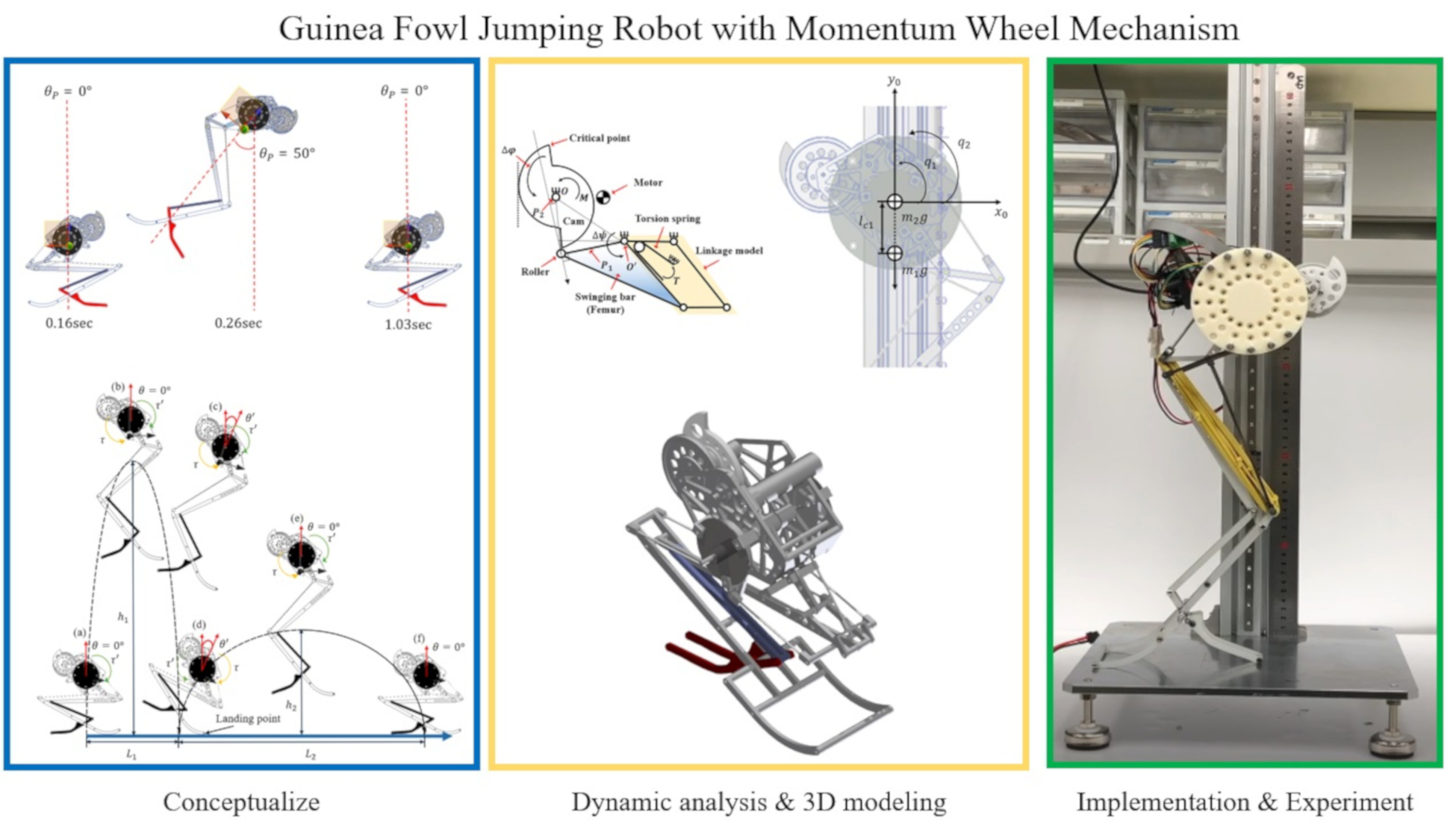
As a result, to design the 1-axis momentum wheel mechanism, we have to consider the torque value that occurs when the robot starts jumping. Figure 5 shows the assumption of the change of the body angle after jumping. ${\mathsf{\theta }}_{\mathrm{p}}$ is the body angle, and the red line is the line connecting C.M. and joint A, and it can be seen that it is perpendicular to the ground. Unlike the jumping experiment, the tilted angle is set to 50 degrees at 0.26 s. The reason for this is that the momentum wheel must be able to control the robot even if the robot’s body is tilted by 50 degrees. Next, to calculate the angular acceleration, we considered the change of time and ${\mathsf{\theta }}_{\mathrm{p}}$ between 0.16 s and 0.26 s. The variation of time is 0.1 s, and the variation of the body angle is 50 degrees. Thus, the angular acceleration of the jumping robot is 43.195 rad/${\mathrm{s}}^2$. We subsequently calculate the moment of inertia using the Autodesk inventor. The value of the moment of inertia of guinea fowl jumping robot is 4519.018 kg ${\mathrm{mm}}^2$.

Using Equation (11), we can calculate the torque value when the robot starts jumping. At this time, if the torque value of the momentum wheel is equal to the torque value generated while jumping, it is possible to cancel the torque. Therefore, our goal is to control the altitude by canceling the torque, and thus we need to adjust the moment of inertia of the momentum wheel. At this time, the angular acceleration of the motor is obtained by dividing the mechanical time constant by 63.2% of the nominal speed, and the value of the maximum angular acceleration of the motor is 10,279 rad/${\mathrm{s}}^2$. In Equation (11), ${\mathrm{I}}_{\max }$ represents the maximum moment of inertia on the y-axis of the robot, and the value is 6678.5 ${\mathrm{kg}\mathrm{mm}}^2$. This is because the moment of inertia is multiplied by 1.5 for the safety factor. ${\mathrm{I}}_{\mathrm{r}}$ is the moment of inertia of the rotor, and the value obtained using the datasheet of the EC45 flat motor is 5.23 ${\mathrm{kg}\mathrm{mm}}^2$. The value of ${\mathsf{\alpha }}_{\mathrm{b}}$ is the angular acceleration of the robot’s body, and this value is 43.195 $\mathrm{rad}/{\mathrm{s}}^2$. ${\mathrm{M}}_{\mathrm{m}}$ is assumed to be 80 g by the weight of the momentum wheel. $\mathrm{r}$ is the radius of the momentum wheel, ${\mathsf{\alpha }}_{\mathrm{m}}$ is the angular acceleration of the motor, and the value of ${\mathsf{\alpha }}_{\mathrm{m}}$ is 10,279 rad/${\mathrm{s}}^2$. The radius of the momentum wheel obtained by substituting the parameter to Equation (11) is 5.1 cm. Salto-1P has an inertial tail mechanism, and the length of the inertial tail is 15 cm. As a result, we see that the momentum wheel mechanism can reduce the volume of the inertial tail mechanism.

$$\mathsf{\tau }=\left({\mathrm{I}}_{\max }+{\mathrm{I}}_{\mathrm{r}}\right){\ast \mathsf{\alpha }}_{\mathrm{b}}=\frac{1}{2}{\mathrm{M}}_{\mathrm{m}}{\mathrm{r}}^2{\ast \mathsf{\alpha }}_{\mathrm{m}},$$

(11)

Next, to verify the performance of the momentum wheel, we design the experiment apparatus as shown in Figure 6a. We fix the jumping robot to the rotating joint with Slider A so that it can test whether the body of the robot moves when the jumping robot activates the momentum wheel. In addition, we can fix Slider A by fixing Slider B. At this time, if Slider B is released, we can perform the jumping experiment using the momentum wheel. As a result, the performance of the momentum wheel can be confirmed by using the experimental apparatus, and the continuous jumping performance of the jumping robot can be tested by releasing Slider B.

Figure 6b is the dynamic model of the jumping robot with the momentum wheel. When $\mathrm{i}=1,2$, $\mathrm{j}=1,2$,${\mathrm{q}}_1$ denotes the body angle of the jumping robot, and ${\mathrm{q}}_2$ is the angle of the inertia wheel. ${\mathrm{m}}_1$ is the mass of the jumping robot, and ${\mathrm{m}}_2$ is the mass of the momentum wheel. ${\mathrm{l}}_1$ is the distance from the anchor to the center of mass of the momentum wheel, ${\mathrm{l}}_{\mathrm{c}1}$ is the distance from the anchor to the center of mass of the jumping robot, ${\mathrm{I}}_1$ is the moment of inertia of the robot, and ${\mathrm{I}}_2$ is the moment of inertia of the inertia wheel.

To calculate the dynamic model, we use the Euler–Lagrange equation, given in Equation (12). The first term of Equation (12) is the kinetic energy part that consists of the translational kinetic energy and rotational kinetic energy part. The second part is Coriolis terms, and the third part is the potential energy part. Our goal is to obtain the inertia matrix by adding the translational kinetic energy and the rotational kinetic energy, and then calculating the Coriolis terms and the potential energy part. These parts will be used to define the control parameters.

$${{\displaystyle \sum }}_{\mathrm{j}}{\mathrm{d}}_{\mathrm{kj}}\ddot{\mathrm{q}}+{{\displaystyle \sum }}_{\mathrm{i},\mathrm{j}}\left\{\frac{\partial {\mathrm{d}}_{\mathrm{kj}}}{\partial {\mathrm{q}}_{\mathrm{i}}}-\frac{1}{2}\frac{\partial {\mathrm{d}}_{\mathrm{ij}}}{\partial {\mathrm{q}}_{\mathrm{k}}}\right\}\dot{{\mathrm{q}}_{\mathrm{i}}}\dot{{\mathrm{q}}_{\mathrm{j}}}-\frac{\partial \mathrm{P}}{\partial {\mathrm{q}}_{\mathrm{k}}}={\mathsf{\tau }}_{\mathrm{k}},$$

(12)

First, to find the inertia matrix $\mathrm{D}\left(\mathrm{q}\right)$, we consider the Jacobian expression ${\mathrm{J}}_{{\mathrm{v}}_{\mathrm{ci}}}$. The results of ${\mathrm{J}}_{{\mathrm{v}}_{\mathrm{ci}}}$ are shown in Equations (13) and (14).

$${\mathrm{J}}_{{\mathrm{v}}_{\mathrm{c}1}}=\left[\begin{array}{cc}\frac{\partial {\mathrm{x}}_1}{\partial {\mathrm{q}}_1}& 0\\ \frac{\partial {\mathrm{y}}_1}{\partial {\mathrm{q}}_1}& 0\\ 0& 0\end{array}\right]=\left[\begin{array}{cc}\frac{\partial \left({\mathrm{l}}_{\mathrm{c}1}{\sin \mathrm{q}}_1\right)}{\partial {\mathrm{q}}_1}& 0\\ \frac{\partial \left({\mathrm{l}}_{\mathrm{c}1}{\cos \mathrm{q}}_1\right)}{\partial {\mathrm{q}}_1}& 0\\ 0& 0\end{array}\right]=\left[\begin{array}{cc}{\mathrm{l}}_{\mathrm{c}1}{\cos \mathrm{q}}_1& 0\\ -{\mathrm{l}}_{\mathrm{c}1}{\sin \mathrm{q}}_1& 0\\ 0& 0\end{array}\right],$$

(13)

$${\mathrm{J}}_{{\mathrm{v}}_{\mathrm{c}2}}=\left[\begin{array}{cc}{\mathrm{l}}_1{\cos \mathrm{q}}_1& 0\\ -{\mathrm{l}}_1{\sin \mathrm{q}}_1& 0\\ 0& 0\end{array}\right],$$

(14)

Then, to calculate the kinetic energy part of Equation (12), we can obtain the translational part of the kinetic energy using Equation (15).

$$\frac{1}{2}\dot{\mathrm{q}}\left\{{\mathrm{m}}_1{\mathrm{J}}_{{\mathrm{v}}_{\mathrm{c}1}}{}^{\mathrm{T}}{\mathrm{J}}_{{\mathrm{v}}_{\mathrm{c}1}}+{\mathrm{m}}_2{\mathrm{J}}_{{\mathrm{v}}_{\mathrm{c}2}}{}^{\mathrm{T}}{\mathrm{J}}_{{\mathrm{v}}_{\mathrm{c}2}}\right\}\dot{\mathrm{q}},$$

(15)

After we calculate the rotational kinetic energy part, we consider the angular velocity terms using Equation (16).

$${\mathsf{\omega }}_1={\dot{\mathrm{q}}}_1\mathrm{k},{\mathsf{\omega }}_2=\left({\dot{\mathrm{q}}}_1+{\dot{\mathrm{q}}}_2\right)\mathrm{k},$$

(16)

When expressed in the base inertial frame, the rotational kinetic energy of the balance control system is then given by Equation (17). Finally, using Equations (15) and (16), we can find the inertia matrix using Equation (18).

$$\frac{1}{2}{\dot{\mathrm{q}}}^{\mathrm{T}}\left\{{\mathrm{I}}_1\left[\begin{array}{cc}1& 0\\ 0& 0\end{array}\right]+{\mathrm{I}}_1\left[\begin{array}{cc}1& 1\\ 1& 1\end{array}\right]\right\}\dot{\mathrm{q}},$$

(17)

$$\begin{array}{ll}\mathrm{D}\left(\mathrm{q}\right)={\mathrm{m}}_1{\mathrm{J}}_{{\mathrm{v}}_{\mathrm{c}1}}{}^{\mathrm{T}}& {\mathrm{J}}_{{\mathrm{v}}_{\mathrm{c}1}}+{\mathrm{m}}_2{\mathrm{J}}_{{\mathrm{v}}_{\mathrm{c}2}}{}^{\mathrm{T}}{\mathrm{J}}_{{\mathrm{v}}_{\mathrm{c}2}}+\left[\begin{array}{cc}{\mathrm{I}}_1+{\mathrm{I}}_2& {\mathrm{I}}_2\\ {\mathrm{I}}_2& {\mathrm{I}}_2\end{array}\right]=\left[\begin{array}{cc}{\mathrm{m}}_1{\mathrm{l}}_{{\mathrm{c}}_1}{}^2+{\mathrm{m}}_2{\mathrm{l}}_1{}^2+{\mathrm{I}}_1+{\mathrm{I}}_2& {\mathrm{I}}_2\\ {\mathrm{I}}_2& {\mathrm{I}}_2\end{array}\right]\\ & =\left[\begin{array}{cc}{\mathrm{d}}_{11}& {\mathrm{d}}_{12}\\ {\mathrm{d}}_{21}& {\mathrm{d}}_{22}\end{array}\right],\end{array}$$

(18)

Next, to find the potential energy term of Equation (12), we can use Equation (19).

$$\mathrm{P}={\mathrm{P}}_1+{\mathrm{P}}_2={\mathrm{m}}_1{\mathrm{gl}}_{\mathrm{c}1}{\cos \mathrm{q}}_1+{\mathrm{m}}_2{\mathrm{gl}}_1{\cos \mathrm{q}}_1,$$

(19)

After finding the potential energy, we can obtain the function of potential energy using Equation (20). The potential energy function is a partial derivative of the potential energy with the angle value.

$${\varnothing }_1=\frac{\partial \mathrm{P}}{\partial {\mathrm{q}}_1}=-{\mathrm{m}}_1{\mathrm{gl}}_{\mathrm{c}1}{\sin \mathrm{q}}_1-{\mathrm{m}}_2{\mathrm{gl}}_1{\sin \mathrm{q}}_1,{\varnothing }_2=0$$

(20)

Next, to calculate the Coriolis term, we consider the Christoffel symbols via Equation (21).

$${\mathrm{c}}_{\mathrm{ijk}}:=\frac{1}{2}\left\{\frac{\partial {\mathrm{d}}_{\mathrm{kj}}}{\partial {\mathrm{q}}_{\mathrm{i}}}+\frac{\partial {\mathrm{d}}_{\mathrm{ki}}}{\partial {\mathrm{q}}_{\mathrm{j}}}-\frac{\partial {\mathrm{d}}_{\mathrm{ij}}}{\partial {\mathrm{q}}_{\mathrm{k}}}\right\},$$

(21)

After calculating the Coriolis terms, we see that the Coriolis terms become zero. We can then obtain Equations (22) and (23).

$${\mathrm{d}}_{11}\ddot{{\mathrm{q}}_1}+{\mathrm{d}}_{12}\ddot{{\mathrm{q}}_2}+\varnothing \left({\mathrm{q}}_1\right)=0,$$

(22)

$${\mathrm{d}}_{21}\ddot{{\mathrm{q}}_1}+{\mathrm{d}}_{22}\ddot{{\mathrm{q}}_2}=\mathsf{\tau }=\mathrm{ki},$$

(23)

In Equation (23), the value of $\mathrm{k}$ denotes the torque constant of the EC motor and the value is 10.4 mNm/A. The value of $\mathrm{i}$ is the current value and it can be controlled by the user up to 2A when using the EPOS24/2 Maxon motor controller. The parameters for obtaining the dynamic model of the guinea fowl jumping robot are shown in

Table 2. The parameter values for calculation of dynamic model.

Symbol	Parameter Value
$\ddot{{\mathrm{q}}_1}$	$43.195\mathrm{rad}/{\mathrm{s}}^2$
${\mathrm{m}}_1$	713 $\mathrm{g}$
${\mathrm{I}}_1$	4519$\mathrm{kg}/{\mathrm{mm}}^2$
${\mathrm{I}}_2$	104.04$\mathrm{kg}/{\mathrm{mm}}^2$
${\mathrm{l}}_{\mathrm{c}1}$	34.011 mm
${\mathrm{l}}_1$	0 mm
${\mathrm{m}}_2$	80$\mathrm{g}$

. Using Equation (23), we can derive Equation (24).

$${\mathrm{q}}_1={\sin }^{-1}\left(\frac{\left({\mathrm{m}}_1{\mathrm{l}}_{\mathrm{c}1}{}^2+{\mathrm{I}}_1+{\mathrm{I}}_2\right)\ddot{{\mathrm{q}}_1}+{\mathrm{I}}_2\ddot{{\mathrm{q}}_2}}{{\mathrm{m}}_1{\mathrm{gl}}_{\mathrm{c}1}}\right),$$

(24)

However, it is difficult to control the body angle by using the angular acceleration of the motor as a variable for controlling the whole system. For this reason, to control the body angle of the jumping robot, the current should be used rather than the acceleration of the motor. As a result, we can obtain Equation (25).

$${\mathrm{q}}_1={\sin }^{-1}\left(\frac{\left({\mathrm{m}}_1{\mathrm{l}}_{\mathrm{c}1}{}^2+{\mathrm{I}}_1+{\mathrm{I}}_2\right)\ddot{{\mathrm{q}}_1}+\mathrm{ki}-{\mathrm{I}}_2\ddot{{\mathrm{q}}_1}}{{\mathrm{m}}_1{\mathrm{gl}}_{\mathrm{c}1}}\right),$$

(25)

3. Experiment Results

In this chapter, we will verify the jumping performance of the guinea fowl jumping robot using the passive and non-passive hallux models and check the performance of the momentum wheel with the jumping robot. Furthermore, we will confirm that the momentum wheel is more stable than the inertial tail through collision simulation.

3.1. Implementation and Jumping Experiment of Guinea Fowl Jumping Robot

The implemented robot is shown in Figure 7a. This figure shows that the robot can withstand using the two digits and hallux despite the load of the robot. In addition, the material of the four torsion springs is SUS304, and we used a latex rubber band on the tibiotarsus to increase the jumping height.

We constructed the experimental environment as shown in Figure 7a to test the jumping performance of the Guinea fowl jumping robot. We supply 9 V to the jumping robot using a power supply. If the robot started jumping, we turned off the motor immediately to prevent the robot from jumping in the air. In addition, to measure the jumping height, we attached a ruler to the table. The results of the jumping test are shown in Figure 7b.

At 0.13 s, the robot still accumulates elastic energy, and we can confirm that the foot of the robot is stably attached to the ground. At 0.26 s, the robot approaches the highest height, and we can confirm that the maximum jumping height is 19.5 cm, as shown in Figure 7. Furthermore, when the robot starts jumping, rotational torque is generated to the robot’s body. For this reason, the foot of the robot tilts forward 42 degrees. Finally, at 1.03 s, the robot tilts forward until 90 degrees and falls to the ground. The experimental results show that the robot can jump vertically up to 19.5 cm and the robot drops to its initial position after the jump. Through the experimental results, we can see that there is a difference of 5.8 cm between the ideal jumping height and the experiment results.

The jumping robot with the non-passive hallux model is shown in Figure 8. As can be seen in the figure, unlike Figure 7a, there is no link structure to support the hallux. To check the performance of the non-passive hallux model, we construct the experiment environment as presented in Figure 8. The robot is 75 cm from the left side of the white board, and the robot maintains the POT stage on the board.

The results of the jumping performance of the non-passive hallux model are shown in Figure 9. At 0.19 s, the digit is lifted because the motor winding speed is too fast. At 0.37 s, the digits are going down and the hallux part is lifted. For this reason, the jumping angle becomes 56 degrees. At 0.56 s, the cam starts to accumulate elastic energy. As a result, the robot begins to change the motion from the POT stage to PRT stage. At 0.82 s, the jumping robot reaches the PRT stage to prepare for the next jump, and we can see that the robot can jump forward 75 cm. Through the experiment, we confirmed that the implemented robot can perform continuous jumping and that it is necessary to construct a passive hallux structure that helps to move the links stably according to the motor winding speed. As a result, through the two jumping experiments above, we can see that the passive hallux model is more stable than the non-passive hallux model.

3.2. Results of Balance Control Experiment

To control the jumping robot, it is necessary to design the electric circuit. The conceptual diagram of the circuit designed to move the DC motor and the EC45 flat motor is shown in Figure 10. Two EPOS24/2 controllers are used, and CAN communication is used. At this time, if the user applies the control signal to the motor driver, both the DC motor and the EC45 flat motor can be controlled using the C# program. At this time, the communication between the EPOS24/2 and PC is serial communication by using a USB interface. The weight of the electric circuit with the momentum wheel is 510 g. Therefore, the jumping robot with the momentum wheel and rotating joint with Slider A is 1603 g. Through Equation (9), we see that the jumping height is 10.8 cm.

Next, the jumping robot fixed on the rotational joint and the rotational joint cannot perform translational motion. However, the jumping robot can perform rotational motion due to the rotational joint. After we set the experiment, we checked how the body angle changes when the angular acceleration of the momentum wheel changes from 0$\mathrm{rad}/{\mathrm{s}}^2$ to 4000 $\mathrm{rad}/{\mathrm{s}}^2$. The experiment results are shown in Figure 11. At 0 s, the momentum wheel starts to rotate, and the body angle of the robot begins to change. At 0.17 s, the body angle tilts up to 43.2 degrees when the angular acceleration of the momentum wheel is 4000 $\mathrm{rad}/{\mathrm{s}}^2$.

Then, we compared the experimental results with the theoretical results. The results are shown in Figure 12. The red line represents the value for the dynamic model, and the blue line gives the experimental results. As shown in Figure 12, when the angular acceleration of the motor increased, the body angle of the robot also increased. Furthermore, the tendency of the experiment results and theoretical results is the same, and the average error rate between the theoretical value and experimental value is 10.85%.

After we checked the performance of the momentum wheel mechanism, we constructed the experiment setup, as shown in Figure 13, to assess how the momentum wheel affects the jumping trajectory. At this time, the linear guide is configured to be able to perform translational motion and rotational motion, and the robot is installed in the rotational joint of the linear guide. First, we wondered what would happen when the robot jumped without operating the momentum wheel, and the results are shown in Figure 13a. At 0 s, the robot maintains the POT stage and the jumping robot is connected to the rotational joint. After 0 s, the robot starts changing the motion from the POT stage to the PRT stage. At 0.24 s, the body angle of the robot tilts forward 50.8 degrees, and the jumping height is 6 cm. At 1.05 s, the foot of the robot falls out of the plate.

Next, we carried out an experiment where the landing point is changed when the robot jumped with the momentum wheel. Figure 13b shows the results of the jumping experiment with the momentum wheel. At 0.89 s, the jumping height is 6.7 cm, and the hallux falls down on the jumping plate at 1.05 s. This is because the momentum wheel mechanism produced the torque in the opposite direction to reduce the body angle change during the takeoff phase.

Through the jumping test with the momentum wheel mechanism, we confirmed that the forward tilting angle decreases, and the robot can land on the plate when the robot jumps. This experiment confirmed that the momentum wheel could contribute to control of the body angle. In addition, through the jumping experiment with and without momentum wheel operation, we observed that the jumping height changed from 6 cm to 6.7 cm. As a result, we confirmed that the momentum wheel could contribute to the altitude control of the jumping robot through the experiment and checked that the jumping height increases when the robot jumps vertically using the momentum wheel.

3.3. Collision Simulation of Momentum Wheel and Inertial Tail

In this section, we will check whether the momentum wheel can have a more compact design than the inertial tail, and we will confirm that the momentum wheel is more stable than the inertial tail through the crash simulation. First, we performed a simulation whereby the momentum wheel could be designed more compactly than the inertial tail. The comparison of the physical characteristics of the momentum wheel and the inertial tail is shown in Figure 14. After fixing the weight and momentum of inertia of the momentum wheel and inertial tail, the diameters of each model were compared. Unlike the general momentum wheel, the proposed momentum wheel is designed to increase the momentum of inertia by concentrating the weight on the edge of the circle. As a result, we were able to design a compact momentum wheel that reduced the diameter of the momentum wheel by 20% compared to the inertial tail.

Next, the simulation environment was configured as shown in Figure 15a for the collision simulation of the momentum wheel and the inertial tail. The jumping robot is standing on the ground in the PRT stage, and an obstacle is placed on the top of the jumping robot. After attaching the momentum wheel and inertial tail to the jumping robot, a simulation of collision with an obstacle while jumping in the air was performed. Through simulation, we analyzed the change of body angle for three axes of the jumping robot and the number of turns during the collision.

The simulation result is shown in Figure 16. Figure 16a–c refer to ${\mathrm{P}}_{\mathrm{x}}$, ${\mathrm{P}}_{\mathrm{y}}$, and ${\mathrm{P}}_{\mathrm{z}}$, respectively, and at 0.23 s, the jumping robot collides with an obstacle. In the case of the inertial tail, the body angle change on the x-axis increases rapidly 5 times higher than the momentum wheel at 0.5 s. In addition, Figure 16b,c show that when the inertial tail collides with the obstacle, the frequency of body angle change is higher than the momentum wheel mechanism by three times. As a result, it can be seen that the proposed momentum wheel is more stable than the inertial tail. However, when comparing the performance of the inertial tail and momentum wheel in a real environment using the one-axis control system, it is hard to accurately compare the two mechanisms when the robot jumps or collides with an obstacle by using the one-axis control system. This is because if there is no three-axis control system for the jumping robot, the balance of the jumping robot keeps changing every time it jumps. In future work, we will implement a three-axis control system and then perform a collision experiment to compare the performance of the inertial tail and momentum wheel accurately.

4. Conclusions

We demonstrate that the guinea fowl jumping robot can perform stable vertical jumping and the momentum wheel mechanism that has a compact design, compared with the inertial tail mechanism, can control the body angle. A jumping robot is implemented by mimicking a guinea fowl to realize the performance of vertical jumping and increase the jumping stability during the initial jumping by using the passive hallux model. In addition, to verify the performance of vertical jumping and the hallux model, a design, simulation, and experiments were conducted. Through the jumping experiments, we verified that the proposed jumping robot can perform vertical jumps and the passive hallux model can contribute to the robot’s more stability when performing the initial jumping. Besides, a momentum wheel mechanism is proposed to create a compact balance control mechanism while maintaining the control performance of the inertial tail mechanism used in the conventional jumping robot. In addition, we verified that the momentum wheel could contribute to the body angle control of the jumping robot through dynamic analysis and an experiment with the momentum wheel. Furthermore, we verified that the momentum wheel can have a more stable and compact design during a collision than the inertial tail through collision simulation. Collision simulation shows that when the inertial tail collides with the obstacle, the frequency of body angle change is higher than the momentum wheel mechanism by three times, and the change of body angle of the inertial tail mechanism is five times higher than the momentum wheel. In addition, a jumping test with the one-axis momentum wheel confirmed that the guinea fowl robot could successfully land after the jump, and this result showed the possibility that the jumping robot with the momentum wheel mechanism could jump continuously. However, to make a precise control model for the posture of the proposed jumping robot model, a three-axis momentum wheel mechanism and closed-loop control using an IMU sensor are required. In future work, we will apply the three-axis balance control system on the guinea fowl jumping robot for the performance of a continuous jump on rough terrain. Besides, we will conduct a collision test to compare the performance of the inertial tail and momentum wheel mechanism in the real environment. We expect that, in future work, the jumping robot with a three-axis momentum wheel mechanism can be used for exploration in various environments.

References

1. Chen, G.; Tu, J.; Ti, X.; Hu, H. A Single-legged Robot Inspired by the Jumping Mechanism of Click Beetles and Its Hopping Dynamics Analysis. J. Bionic Eng. 2020, 17, 1109–1125. [Google Scholar] [CrossRef]
2. Lo, J.; Parslew, B. An Energetic Analysis of Rhomboidal Linkage Robots for Hopping Lunar Exploration. In Proceedings of the 2021 Second International Symposium on Instrumentation, Control, Artificial Intelligence, and Robotics (ICA-SYMP), Bangkok, Thailand, 20–22 January 2021; pp. 1–5. [Google Scholar]
3. Ma, Y.; Wei, Y.; Kong, D. A Biologically Inspired Height-Adjustable Jumping Robot. Appl. Sci. 2021, 11, 5167. [Google Scholar] [CrossRef]
4. Shun, G. Locomotion Identification Method of One-Degree-of-Freedom Six-Bar for Jumping Robot. J. Mech. Robot. 2022, 14, 031008. [Google Scholar]
5. Yu, Z.; Zeng, Y.; Guo, C. Mechanical Design and Performance Analysis of a Weevil-Inspired Jumping Mechanism. Machines 2022, 10, 161. [Google Scholar] [CrossRef]
6. Yun, D. Development of a mobile robot mimicking the frilled lizard. J. Mech. Sci. Technol. 2018, 32, 1787–1792. [Google Scholar] [CrossRef]
7. Zhang, Z.; Chang, B.; Zhao, J.; Yang, Q.; Liu, X. Design, optimization, and experiment on a bioinspired jumping robot with a six-bar leg mechanism based on jumping stability. Math. Probl. Eng. 2020, 2020, 3507203. [Google Scholar] [CrossRef]
8. Zhao, J.; Zhao, T.; Xi, N.; Mutka, M.W.; Xiao, L. MSU tailbot: Controlling aerial maneuver of a miniature-tailed jumping robot. IEEE/ASME Trans. Mechatron. 2015, 20, 2903–2914. [Google Scholar] [CrossRef]
9. Zhang, J.; Song, G.; Li, Y.; Qiao, G.; Song, A.; Wang, A. A bio-inspired jumping robot: Modeling, simulation, design, and experimental results. Mechatronics 2013, 23, 1123–1140. [Google Scholar] [CrossRef]
10. Fukushima, T.; Siddall, R.; Schwab, F.; Toussaint, S.L.D.; Byrnes, G.; Nyakatura, J.A.; Jusufi, A. Inertial Tail Effects during Righting of Squirrels in Unexpected Falls: From Behavior to Robotics. Integr. Comp. Biol. 2021, 61, 589–602. [Google Scholar] [CrossRef]
11. Butt, J.M.; Chu, X.; Zheng, H.; Wang, X.; Kwok, K.-W.; Au, K.S. Modeling and Control of Soft Robotic Tail Based Aerial Maneuvering (STAM) System: Towards Agile Self-Righting with a Soft Tail. In Proceedings of the 2021 20th International Conference on Advanced Robotics (ICAR), Ljubljana, Slovenia, 6–10 December 2021; pp. 531–538. [Google Scholar]
12. Tsuda, T.; Mochiyama, H.; Fujimoto, H. Robotic jerboa: A compact bipedal kick-and-slide robot powered by unidirectional impulse force generators. In Proceedings of the 2010 IEEE/RSJ International Conference on Intelligent Robots and Systems, Taipei, Taiwan, 18–22 October 2010; pp. 2523–2524. [Google Scholar]
13. Yim, J.K.; Singh, B.R.P.; Wang, E.K.; Featherstone, R.; Fearing, R.S. Precision robotic leaping and landing using stance-phase balance. IEEE Robot. Autom. Lett. 2020, 5, 3422–3429. [Google Scholar] [CrossRef]
14. Kim, M.; Song, B.; Yun, D. Study on Guinea Fowl Mimicking Jumping Robot with Momentum Wheel Mechanism. In Proceedings of the 2021 24th International Conference on Mechatronics Technology (ICMT), Singapore, 18–22 December 2021; pp. 1–6. [Google Scholar]
15. Kim, M.; Yun, D. Guinea fowl Jumping Robot with Balance Control Mechanism: Modeling, simulation, and experiment results. In Proceedings of the 2019 IEEE/RSJ International Conference on Intelligent Robots and Systems (IROS), Macau, China, 3–8 November 2019; pp. 779–786. [Google Scholar]
16. Henry, H.T.; Ellerby, D.J.; Marsh, R.L. Performance of guinea fowl Numida meleagris during jumping requires storage and release of elastic energy. J. Exp. Biol. 2005, 208, 3293–3302. [Google Scholar] [CrossRef] [PubMed] [Green Version]
17. McGowan, C.P.; Duarte, H.A.; Main, J.B.; Biewener, A.A. Effects of load carrying on metabolic cost and hindlimb muscle dynamics in guinea fowl (Numida meleagris). J. Appl. Physiol. 2006, 101, 1060–1069. [Google Scholar] [CrossRef] [PubMed] [Green Version]
18. Rubenson, J.; Henry, H.T.; Dimoulas, P.M.; Marsh, R.L. The cost of running uphill: Linking organismal and muscle energy use in guinea fowl (Numida meleagris). J. Exp. Biol. 2006, 209, 2395–2408. [Google Scholar] [CrossRef] [PubMed] [Green Version]
19. Rubenson, J.; Marsh, R.L. Mechanical efficiency of limb swing during walking and running in guinea fowl (Numida meleagris). J. Appl. Physiol. 2009, 106, 1618–1630. [Google Scholar] [CrossRef] [PubMed] [Green Version]
20. Weiss, A.; Zaitsev, V.; Nabi, N.; Hanan, U.B. Landing recovery and orientation control of a locust-inspired miniature jumping robot. Eng. Res. Express 2020, 2, 015017. [Google Scholar] [CrossRef]
21. Mukhayadi, M. Efficient and High Precision Momentum Bias Attitude Control for Small Satellite. Ph.D. Thesis, Technische Universität Berlin, Berlin, Germany, 2021. [Google Scholar]
22. Yoon, H. Maximum Reaction-Wheel Array Torque/Momentum Envelopes for General Configurations. J. Guid. Control Dyn. 2021, 44, 1219–1223. [Google Scholar] [CrossRef]
Figure 1. Linkage model of guinea fowl jumping robot with passive hallux model.
Electronics 11 01191 g001
Figure 2. Simulation result of passive hallux model and non-passive hallux model: (a) closed loop model of non-passive hallux model; (b) non-passive hallux model; (c) Simulation results of non-passive and passive hallux model.
Electronics 11 01191 g002
Figure 3. Design of trigger mechanism: (a) Dynamic model of trigger mechanism; (b) 3D modeling of trigger mechanism with passive hallux model; (c) Coordinates of the center of mass when PRT and POT.
Electronics 11 01191 g003
Figure 4. The balance control mechanism of the guinea fowl jumping robot using one-axis momentum wheel: (a) Stance phase with balance control; (b) Control of body angle at maximum jumping height; (c) Tilting control for stable landing; (d) Landing and takeoff angle control for next jumping; (e) Control of body angle at maximum jumping height on second jumping; (f) Landing.
Electronics 11 01191 g004
Figure 5. Assumption of vertical jumping. At 0.16 s, the robot changes from the POT stage to the PRT stage and the body angle tilts forward 50 degrees at 0.26 s. The robot can stand at 1.03 s due to the momentum wheel mechanism.
Electronics 11 01191 g005
Figure 6. Schematic of guinea fowl jumping robot with 1-axis momentum wheel: (a) 3D modeling of experiment apparatus with a jumping robot; (b) Dynamic model of 1-axis momentum wheel mechanism.
Electronics 11 01191 g006
Figure 7. The experiment of guinea fowl jumping robot: (a) Implementation of jumping robot; (b) Jumping experiment without momentum wheel.
Electronics 11 01191 g007
Figure 8. The experiment setting of the non-passive model.
Electronics 11 01191 g008
Figure 9. Jumping results of non-passive hallux model; The forward jumping angle is 56 degrees, and the robot can jump forward 75 cm.
Electronics 11 01191 g009
Figure 10. Design of control circuit of guinea fowl jumping robot with momentum wheel mechanism.
Electronics 11 01191 g010
Figure 11. The experiment of momentum wheel mechanism. At 0.17 s, the maximum value of body angle is 43.2 degrees.
Electronics 11 01191 g011
Figure 12. Relationship between body angle of jumping robot and angular acceleration of momentum wheel.
Electronics 11 01191 g012
Figure 13. Jumping experiment with momentum wheel mechanism: (a) Jumping experiment without momentum wheel; (b) Jumping experiment with momentum wheel.
Electronics 11 01191 g013
Figure 14. Comparison of physical properties for momentum wheel and inertial tail: (a) Momentum wheel; (b) Inertial tail.
Electronics 11 01191 g014
Figure 15. Collision simulation: (a) Simulation setting of collision; (b) Collision simulation result of momentum wheel mechanism; (c) Collision simulation result of inertial tail mechanism.
Electronics 11 01191 g015
Figure 16. Results of collision simulation: (a) Change of body angle ( P x ); (b) Change of body angle ( P y ); (c) Change of body angle ( P z ).
Electronics 11 01191 g016