A Hybrid Predictive Type-3 Fuzzy Control for Time-Delay Multi-Agent Systems

Abstract

In this paper, the consensus problem is addressed for multi-agent systems. The dynamics of each agent contain unknown uncertain/nonlinear terms and unknown time delays. A type-3 fuzzy logic system is developed to tackle the effect of unknown dynamics and design a hybrid controller. The policy scheme involves two control signals for the stabilization of the approximation and consensus error of each agent dynamic. To this end, based on the concept of the model predictive control approach, the constrained control laws are designed and updated at each time step. The simulations results portray the error signals. Feasibility, appropriate convergence, and proper transient response are the main merits of the suggested method.

1. Introduction

1.1. Literature Review

Multi-agent systems (MASs) have been the focus of a variety of research papers because of their extensive applications in diverse fields [1]. For instance, a formation control scenario based on an event-triggered scheme was developed for MASs and the effect of mixed measurements was studied in [2]. A distributed protocol containing a controller and a filter was applied to a group of double integrator agents to study the tracking problem in [3]. In another paper, a distributed adaptive policy was suggested to analyze MASs subject to sensor attacks [4]. Moreover, a distributed consensus of linear MASs with matching uncertainties was analyzed in [5].

In the case of heterogeneous discrete-time MASs, the output synchronization issue was investigated via an adaptive distributed observer [6]. The cooperative control of non-identical double-integrators with parameter uncertainties was studied in [7]. The problem of the output synchronization of heterogeneous/homogenous linear MASs was studied via output feedback controllers in [8]. In another paper, a distributed resilient controller was designed to tackle sensor faults/attacks and study the ultimate boundedness of heterogeneous MASs [9]. The authors used a model predictive control (MPC) approach for the consensus of MASs in [10]. Recently, the synchronization problem of MASs subject to disturbances was investigated in [11]. Moreover, this same problem was addressed when a system sufferred from input time delay [12]. The fault-tolerant control of heterogeneous MASs was studied by considering a virtual actuator in [13].

On the other hand, neural and fuzzy logic system (FLS) -based control approaches have been extensively applied for uncertain applications [14,15,16]. For instance, in [17] an FLS with optimal secondary fuzzy sets is developed for the frequency control of uncertain microgrids. In [18], the FLS-based synchronization scheme was presented for chaotic systems, and an improvement in the synchronization accuracy of an FLS-based controller was verified. A dynamic programming controller involving the use of FLSs was introduced in [19], and the ability of FLSs to deal with uncertainties was examined. The paper [20] also surveyed type-2 FLSs and fuzzy sets. A deep learning FLS was designed in [21], and the improvement of the estimation ability of FLS was demonstrated. In [22], it was proven that high-order FLSs are more effective in control problems that include uncertainties and noisy faults. More recently, T3-FLSs were described [23]; these provide a better efficiency in various noisy applications. In addition, the reinforcement learning (RL) approach was utilized to compute output synchronization protocols to achieve cooperative output regulation in [24]. The implementation of an adaptive distributed observer along with RL was studied in [25]. Based on the linear matrix inequality (LMI), deep T2-FLS, and restricted Boltzmann machine (RMB) schemes, the leader following of fractional-order MASs in the presence of unknown dynamics was studied in [26]. A distributed FLS-based control technique was suggested for the output consensus of heterogeneous stochastic MASs [27]. For the case of second-order MASs, a backstepping scheme and a distributed observer were proposed for analyzing the consensus in [28]. Utilizing FLSs and a distributed fault-tolerant protocol, a consensus of nonlinear heterogeneous-switched MASs was studied in [29]. Based on a neuro-fuzzy control scheme and a high-gain observer, the synchronization of heterogeneous MASs was investigated in [30]. Based on a polynomial fuzzy modeling approach, the consensus of MASs under switching topologies was ensured in [31].

1.2. Motivations and Objectives

The consensus problem has been well studied for linear homogenous MASs with undirected graphs in the literature. Despite the novel developments in the consensus problem of MASs, research on the consensus problem of heterogeneous MASs with nonlinear dynamics, which involve the characterization of MASs in practical applications, is limited. A review of the existing approaches demonstrates that:

• MASs with time-delay perturbations and uncertain dynamic models have rarely been studied.
• In most studies, distributed control policies have been designed for MASs with known dynamics and only some parametric uncertainties are considered.
• Most of the aforementioned works study linear MASs or the dynamics of the nodes are considered to be Lipschitz type.
• Among all the existing studies, type-3 FLS-based controllers have not been developed for heterogeneous MASs.

1.3. Main Contributions

Motivated by the above literature investigation, in this paper an optimized FLS-based controller is suggested to address heterogeneous nonlinear MASs with time-delay perturbations and uncertain dynamic models. To this end, a type-3 (T3) FLS is established to address the nonlinearities and perturbations. The novel features of this paper are as follows:

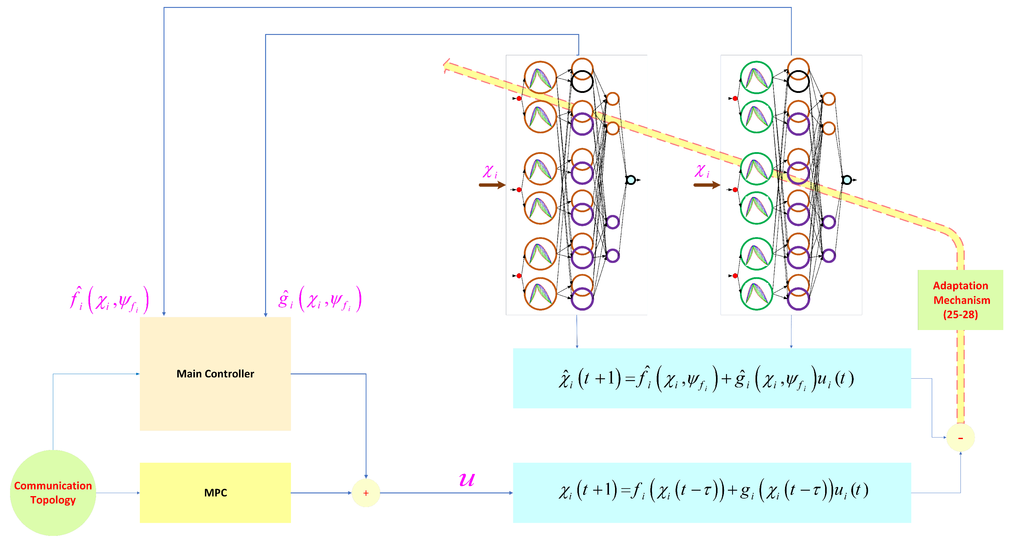
• Based on a compact form of the agent dynamics, the consensus problem of MASs with time delays, heterogeneous structures, unknown dynamic models, and nonlinear terms is analyzed via a novel distributed learning-based control policy.
• An error dynamic system is established for the consensus problem and the stability/robustness analysis of the error dynamics is investigated via an appropriate Lyapunov–Krasovskii functional.
• The optimization problem in the framework of LMIs is suggested and the solution to the optimization problem leads to the gain of a distributed controller.
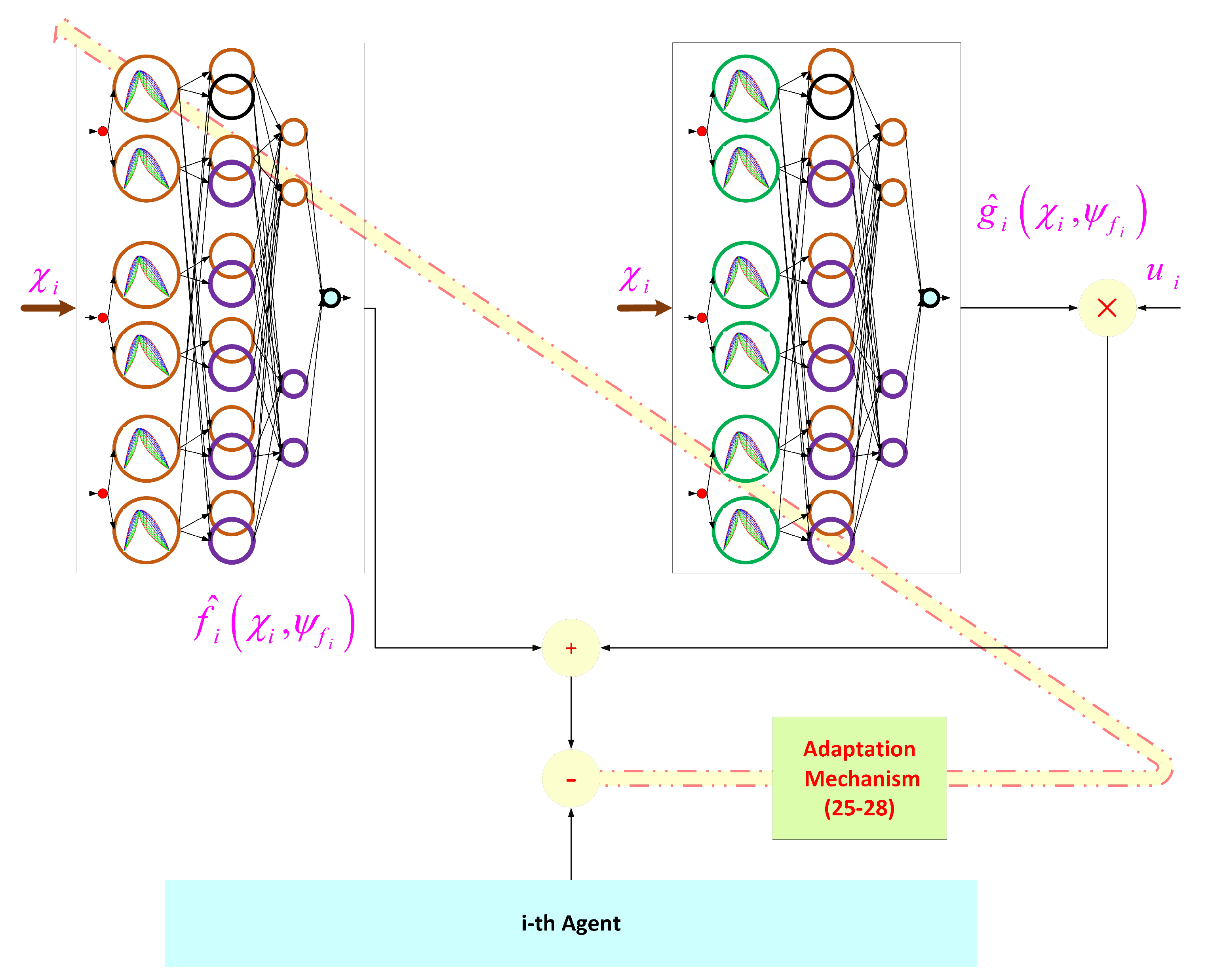
• Type-3 FLS of [23] is formulated to study the nonlinearities of heterogeneous MASs and design a novel hybrid controller. It should be noted that the type-3 FLS-based control of MASs with the aforementioned perturbations has not been studied. In addition, novel online tuning rules for T3-FLS are presented in this paper.

2. Preliminaries and Problem Definition

2.1. Graph Theory

The interaction among all agents is denoted by graph G. The properties of the graph are expressed by $G\left(V,E,\Theta \right)$, where $V=\{0,1,\cdots ,\ell \}$ represents the node set, $E\subseteq V\times V\left\{\right(i,j)\in V\times V\}$ are the edge sets (where the pair of $(i,j)\in E$ if the interaction channel between node i and node j exists, where node j is the neighbour of node i, or in other words agent i can obtain data from the agent j, else $(i,j)⊈E$), and $\Theta =\left[{\theta }_{ij}\right]\in R^{\ell \times \ell }$ is the weighted adjacency matrix. For element ${\theta }_{ij}$ of adjacency matrix $\Theta$, it is defined that ${\theta }_{ii}=0$, ${\theta }_{ij}>0$ if $(i,j)\in E$, and ${\theta }_{ij}=0$ otherwise.

2.2. Problem Definition

The dynamics of the $i\mathrm{-th}$ agent are given as:

$$\begin{array}{c}\hfill {\chi }_i\left(t+1\right)=f_i\left({\chi }_i\left(t-\tau \right)\right)+g_i\left({\chi }_i\left(t-\tau \right)\right)u_i\left(t\right),i=1,\dots ,\ell \end{array}$$

(1)

where $f_i\left({\chi }_i\left(t-\tau \right)\right)$ and $g_i\left({\chi }_i\left(t-\tau \right)\right)$ are unknown functions and $\tau$ is an unknown time-delay. $f_i\left({\chi }_i\left(t-\tau \right)\right)$ and $g_i\left({\chi }_i\left(t-\tau \right)\right)$ are approximated online by suggested T3-FLSs as ${\widehat{f}}_i\left({\chi }_i,{\psi }_{f_i}\right)$ and ${\widehat{g}}_i\left({\chi }_i,{\psi }_{g_i}\right)$, respectively. ${\psi }_{f_i}$ and ${\psi }_{g_i}$ are tunable parameters of ${\widehat{f}}_i\left({\chi }_i,{\psi }_{f_i}\right)$ and ${\widehat{g}}_i\left({\chi }_i,{\psi }_{g_i}\right)$, respectively. Then, the estimation of (1) is written as:

$${\widehat{\chi }}_i\left(t+1\right)={\widehat{f}}_i\left({\chi }_i,{\psi }_{f_i}\right)+{\widehat{g}}_i\left({\chi }_i,{\psi }_{f_i}\right)u_i\left(t\right),i=1,\dots ,\ell$$

(2)

The general scheme of the controller is depicted in Figure 1. The control signal $u_i\left(t\right)$ is written as $u_i\left(t\right)=u_{1i}\left(t\right)+u_{2i}\left(t\right)$. $u_{1i}\left(t\right)$ is designed as:

$$\begin{array}{c}\hfill u_{1i}\left(t\right)={\widehat{g}}_i^{-1}\left({\chi }_i\left(t\right),{\psi }_{g_i}\left(t\right)\right)\left[-{\widehat{f}}_i\left({\chi }_i\left(t\right),{\psi }_{f_i}\left(t\right)\right)+A_i{\chi }_i\left(t\right)\right]\end{array}$$

(3)

where $A_i$ is considered as:

$$\begin{array}{c}\hfill A_i=\left[\begin{array}{cccc}0& 1& \cdots & 0\\ ⋮& ⋮& \cdots & ⋮\\ 0& 0& \cdots & 1\\ -{\lambda }_{i,1}& -{\lambda }_{i,2}& \cdots & -{\lambda }_{i,n}\end{array}\right]\end{array}$$

(4)

where n is the states number in agents and ${\lambda }_i,j,j=1,\dots ,n$ are constants, which are determined such that the Hurwitz stability criterion is satisfied. Then, the dynamics of $i\mathrm{-th}$ agent are written as:

$$\begin{array}{c}\hfill \begin{array}{c}{\chi }_i\left(t+1\right)=A_i{\chi }_i\left(t\right)+{\beta }_i{u}_{2i}\left(t\right)\hfill \\ +\left[f_i\left({\chi }_i\left(t-\tau \right)\right)-{\widehat{f}}_i\left({\chi }_i\left(t\right),{\psi }_{f_i}\left(t\right)\right)\right.\hfill \\ +\left.g_i\left({\chi }_i\left(t-\tau \right)\right)-{\widehat{g}}_i\left({\chi }_i\left(t\right),{\psi }_{g_i}\left(t\right)\right)u_i\left(t\right)\right],i=1,\dots ,\ell \hfill \end{array}\end{array}$$

(5)

By defining the approximation error (AE) as:

$$\begin{array}{c}\hfill \begin{array}{c}{\delta }_i\left(t\right)=\left[f_i\left({\chi }_i\left(t-\tau \right)\right)-{\widehat{f}}_i\left({\chi }_i\left(t\right),{\psi }_{f_i}\left(t\right)\right)\right.\hfill \\ +\left.g_i\left({\chi }_i\left(t-\tau \right)\right)-{\widehat{g}}_i\left({\chi }_i\left(t\right),{\psi }_{g_i}\left(t\right)\right)u_i\left(t\right)\right],\hfill \end{array}\end{array}$$

(6)

it can be found that:

$$\begin{array}{c}\hfill {\chi }_i\left(t+1\right)=A_i{\chi }_i\left(t\right)+{\delta }_i\left(t\right)+{\beta }_i{u}_{2i}\left(t\right),i=1,\dots ,\ell \end{array}$$

(7)

where ${\beta }_i={\left[0,\dots ,1\right]}^T$. AE is written as:

$$\begin{array}{c}\hfill {\delta }_i\left(t\right)=A_{di}{\chi }_i\left(t-d\right)\end{array}$$

(8)

where d is the unknown bounded constant and $A_{di}$ is a known matrix. Then, from (7) and (8), we can obtain:

$$\begin{array}{c}\hfill {\chi }_i\left(t+1\right)=A_i{\chi }_i\left(t\right)+A_{di}{\chi }_i\left(t-d\right)+{\beta }_i{u}_{2i}\left(t\right),i=1,\dots ,\ell \end{array}$$

(9)

The consensus error is defined as:

$$\begin{array}{c}\hfill e_i\left(t\right)={\chi }_i\left(t\right)-\frac{1}{\ell }\sum _{j=1}^{\ell }{\theta }_{ij}{\chi }_j\left(t\right),i=1,\cdots ,\ell \end{array}$$

(10)

Considering (9) and (10), one has:

$$\begin{array}{cc}\hfill & e_i(t+1)={\chi }_i(t+1)-\frac{1}{\ell }\sum _{j=1}^{\ell }{\theta }_{ij}{\chi }_j(t+1),i=1,\cdots ,\ell \hfill \\ \hfill & =A_i{\chi }_i\left(t\right)+A_{di}{\chi }_i\left(t-d\right)+{\beta }_i{u}_{2i}\left(t\right)-\frac{1}{\ell }\sum _{j=1}^{\ell }{\theta }_{ij}\left(A_j{\chi }_j\left(t\right)+A_{dj}{\chi }_j\left(t-d\right)+{\beta }_j{u}_{2j}\left(t\right)\right)\hfill \end{array}$$

(11)

As expressed before, the coefficients ${\theta }_{ij}$ are acquired from the adjacency matrix $\Theta$.

3. Type-3 FLS

The T3-FLS [23] is formulated to cope with uncertainties. In this paper, the new learning laws for optimizing the rules of T3-FLSs are utilized. In addition, the new designed rules are to be used in our online control scheme. Note that two T3-FLSs are used for the online modeling of each agent. The identification and learning structure is shown in Figure 2. The details and learning computations are explained as follows.

(1) The inputs are ${\chi }_i,i=1,\dots ,n$.

(2) Consider $j\mathrm{-th}$ fuzzy set (FS) for ${\chi }_i$ as ${\tilde{\Psi }}_i^j$. Then, the memberships for ${\tilde{\Psi }}_i^j$ at the levels ${\underline{q}}_{\kappa }$ and ${\overline{q}}_{\kappa }$ are written as [23]:

$${\overline{\mathrm{M}}}_{{\tilde{\Psi }}_{i|{\overline{q}}_{\kappa }}^j}=\left\{\begin{array}{c}1-{\left(\frac{\left|{\chi }_i-C_{{\tilde{\Psi }}_i^j}\right|}{{\underline{\Delta }}_{{\tilde{\Psi }}_i^j}}\right)}^{{\overline{q}}_{\kappa }}if{C}_{{\tilde{\Psi }}_i^j}-{\underline{\Delta }}_{{\tilde{\Psi }}_i^j}<{\chi }_i\le C_{{\tilde{\Psi }}_i^j}\\ 1-{\left(\frac{\left|{\chi }_i-C_{{\tilde{\Psi }}_i^j}\right|}{{\overline{\Delta }}_{{\tilde{\Psi }}_i^j}}\right)}^{{\overline{q}}_{\kappa }}if{C}_{{\tilde{\Psi }}_i^j}<{\chi }_i\le C_{{\tilde{\Psi }}_i^j}+{\overline{\Delta }}_{{\tilde{\Psi }}_i^j}\\ 0if{\chi }_i>C_{{\tilde{\Psi }}_i^j}+{\overline{\Delta }}_{{\tilde{\Psi }}_i^j}or{\chi }_i\le C_{{\tilde{\Psi }}_i^j}-{\underline{\Delta }}_{{\tilde{\Psi }}_i^j}\end{array}\right.$$

(12)

$${\overline{\mathrm{M}}}_{{\tilde{\Psi }}_{i|{\underline{q}}_{\kappa }}^j}=\left\{\begin{array}{c}1-{\left(\frac{\left|{\chi }_i-C_{{\tilde{\Psi }}_i^j}\right|}{{\underline{\Delta }}_{{\tilde{\Psi }}_i^j}}\right)}^{{\underline{q}}_{\kappa }}if{C}_{{\tilde{\Psi }}_i^j}-{\underline{\Delta }}_{{\tilde{\Psi }}_i^j}<{\chi }_i\le C_{{\tilde{\Psi }}_i^j}\\ 1-{\left(\frac{\left|{\chi }_i-C_{{\tilde{\Psi }}_i^j}\right|}{{\overline{\Delta }}_{{\tilde{\Psi }}_i^j}}\right)}^{{\underline{q}}_{\kappa }}if{C}_{{\tilde{\Psi }}_i^j}<{\chi }_i\le C_{{\tilde{\Psi }}_i^j}+{\overline{\Delta }}_{{\tilde{\Psi }}_i^j}\\ 0if{\chi }_i>C_{{\tilde{\Psi }}_i^j}+{\overline{\Delta }}_{{\tilde{\Psi }}_i^j}or{\chi }_i\le C_{{\tilde{\Psi }}_i^j}-{\underline{\Delta }}_{{\tilde{\Psi }}_i^j}\end{array}\right.$$

(13)

$${\underline{\mathrm{M}}}_{{\tilde{\Psi }}_{i|{\overline{q}}_{\kappa }}^j}=\left\{\begin{array}{c}1-{\left(\frac{\left|{\chi }_i-C_{{\tilde{\Psi }}_i^j}\right|}{{\underline{\Delta }}_{{\tilde{\Psi }}_i^j}}\right)}^{\frac{1}{{\overline{q}}_{\kappa }}}if{C}_{{\tilde{\Psi }}_i^j}-{\underline{\Delta }}_{{\tilde{\Psi }}_i^j}<{\chi }_i\le C_{{\tilde{\Psi }}_i^j}\\ 1-{\left(\frac{\left|{\chi }_i-C_{{\tilde{\Psi }}_i^j}\right|}{{\overline{\Delta }}_{{\tilde{\Psi }}_i^j}}\right)}^{\frac{1}{{\overline{q}}_{\kappa }}}if{C}_{{\tilde{\Psi }}_i^j}<{\chi }_i\le C_{{\tilde{\Psi }}_i^j}+{\overline{\Delta }}_{{\tilde{\Psi }}_i^j}\\ 0if{\chi }_i>C_{{\tilde{\Psi }}_i^j}+{\overline{\Delta }}_{{\tilde{\Psi }}_i^j}or{\chi }_i\le C_{{\tilde{\Psi }}_i^j}-{\underline{\Delta }}_{{\tilde{\Psi }}_i^j}\end{array}\right.$$

(14)

$${\underline{\mathrm{M}}}_{{\tilde{\Psi }}_{i|{\underline{q}}_{\kappa }}^j}=\left\{\begin{array}{c}1-{\left(\frac{\left|{\chi }_i-C_{{\tilde{\Psi }}_i^j}\right|}{{\underline{\Delta }}_{{\tilde{\Psi }}_i^j}}\right)}^{\frac{1}{{\underline{q}}_{\kappa }}}if{C}_{{\tilde{\Psi }}_i^j}-{\underline{\Delta }}_{{\tilde{\Psi }}_i^j}<{\chi }_i\le C_{{\tilde{\Psi }}_i^j}\\ 1-{\left(\frac{\left|{\chi }_i-C_{{\tilde{\Psi }}_i^j}\right|}{{\overline{\Delta }}_{{\tilde{\Psi }}_i^j}}\right)}^{\frac{1}{{\underline{q}}_{\kappa }}}if{C}_{{\tilde{\Psi }}_i^j}<{\chi }_i\le C_{{\tilde{\Psi }}_i^j}+{\overline{\Delta }}_{{\tilde{\Psi }}_i^j}\\ 0if{\chi }_i>C_{{\tilde{\Psi }}_i^j}+{\overline{\Delta }}_{{\tilde{\Psi }}_i^j}or{\chi }_i\le C_{{\tilde{\Psi }}_i^j}-{\underline{\Delta }}_{{\tilde{\Psi }}_i^j}\end{array}\right.$$

(15)

where ${\overline{\mathrm{M}}}_{{\tilde{\Psi }}_{i|{\overline{q}}_{\kappa }}^j}$/${\overline{\mathrm{M}}}_{{\tilde{\Psi }}_{i|{\underline{q}}_{\kappa }}^j}$ and ${\underline{\mathrm{M}}}_{{\tilde{\Psi }}_{i|{\overline{q}}_{\kappa }}^j}$/${\underline{\mathrm{M}}}_{{\tilde{\Psi }}_{i|{\underline{q}}_{\kappa }}^j}$ denote the upper/lower memberships for ${\tilde{\Psi }}_i^j$ at levels ${\underline{q}}_{\kappa }$ and ${\overline{q}}_{\kappa }$. $C_{{\tilde{\Psi }}_i^j}$ denotes the center of $C_{{\tilde{\Psi }}_i^j}$ and ${\underline{\Delta }}_{{\tilde{\Psi }}_i^j}$ and ${\overline{\Delta }}_{{\tilde{\Psi }}_i^j}$ are the distances of $C_{{\tilde{\Psi }}_i^j}$ to the left/right points of ${\tilde{\Psi }}_i^j$ (see Figure 3).

(3) The rule firings at ${\underline{q}}_{\kappa },{\overline{q}}_{\kappa }$, are:

$${\overline{\varphi }}_{{\overline{q}}_{\kappa }}^l={\overline{\mathrm{M}}}_{{\tilde{\Psi }}_{1|{\overline{q}}_{\kappa }}^{p_1}}·{\overline{\mathrm{M}}}_{{\tilde{\Psi }}_{1|{\overline{q}}_{\kappa }}^{p_2}}\cdots {\overline{\mathrm{M}}}_{{\tilde{\Psi }}_{1|{\overline{q}}_{\kappa }}^{p_n}}$$

(16)

$${\overline{\varphi }}_{{\underline{q}}_{\kappa }}^l={\overline{\mathrm{M}}}_{{\tilde{\Psi }}_{1|{\underline{q}}_{\kappa }}^{p_1}}·{\overline{\mathrm{M}}}_{{\tilde{\Psi }}_{1|{\underline{q}}_{\kappa }}^{p_2}}\cdots {\overline{\mathrm{M}}}_{{\tilde{\Psi }}_{1|{\underline{q}}_{\kappa }}^{p_n}}$$

(17)

$${\underline{\varphi }}_{{\overline{q}}_{\kappa }}^l={\underline{\mathrm{M}}}_{{\tilde{\Psi }}_{1|{\overline{q}}_{\kappa }}^{p_1}}·{\underline{\mathrm{M}}}_{{\tilde{\Psi }}_{1|{\overline{q}}_{\kappa }}^{p_2}}\cdots {\underline{\mathrm{M}}}_{{\tilde{\Psi }}_{1|{\overline{q}}_{\kappa }}^{p_n}}$$

(18)

$${\underline{\varphi }}_{{\underline{q}}_{\kappa }}^l={\underline{\mathrm{M}}}_{{\tilde{\Psi }}_{1|{\underline{q}}_{\kappa }}^{p_1}}·{\underline{\mathrm{M}}}_{{\tilde{\Psi }}_{1|{\underline{q}}_{\kappa }}^{p_2}}\cdots {\underline{\mathrm{M}}}_{{\tilde{\Psi }}_{1|{\underline{q}}_{\kappa }}^{p_n}}$$

(19)

where the $l\mathrm{-th}$ rule is:

$$\begin{array}{c}l\mathrm{-th}Rule:\hfill \\ if{\chi }_{1}is{\tilde{\Psi }}_1^{p_1}and{\chi }_{2}is{\tilde{\Psi }}_2^{p_2}and\cdots {\chi }_{n}is{\tilde{\Psi }}_n^{p_n}\hfill \\ Theny\in \left[{\underline{\omega }}_l,{\overline{\omega }}_l\right],l=1,\dots ,M\hfill \end{array}$$

(20)

where ${\tilde{\Psi }}_i^{p_j}$ is the $p_j\mathrm{-th}$ FS for input ${\chi }_i$ and ${\underline{\omega }}_l$ and ${\overline{\omega }}_l$ denote the rule parameters, which are optimized.

(4) The output is written as:

$$y=\sum _{\kappa =1}^K\left({\underline{q}}_{\kappa }{\underline{y}}_{\kappa }+{\overline{q}}_{\kappa }{\overline{y}}_{\kappa }\right)/\phantom{\sum _{\kappa =1}^K\left({\underline{q}}_{\kappa }{\underline{y}}_{\kappa }+{\overline{q}}_{\kappa }{\overline{y}}_{\kappa }\right)\sum _{\kappa =1}^K\left({\underline{q}}_{\kappa }+{\overline{q}}_{\kappa }\right)}\sum _{\kappa =1}^K\left({\underline{q}}_{\kappa }+{\overline{q}}_{\kappa }\right)$$

(21)

where:

$${\overline{y}}_{\kappa }=\frac{{\displaystyle \sum _{l=1}^{n_r}}\left({\overline{\varphi }}_{{\overline{q}}_{\kappa }}^l{\overline{\omega }}_l+{\underline{\varphi }}_{{\overline{q}}_{\kappa }}^l{\underline{\omega }}_l\right)}{{\displaystyle \sum _{l=1}^{n_r}}\left({\overline{\varphi }}_{{\overline{q}}_{\kappa }}^l+{\underline{\varphi }}_{{\overline{q}}_{\kappa }}^l\right)}$$

(22)

$${\underline{y}}_{\kappa }=\frac{{\displaystyle \sum _{l=1}^{n_r}}\left({\overline{\varphi }}_{{\underline{q}}_{\kappa }}^l{\overline{\omega }}_l+{\underline{\varphi }}_{{\underline{q}}_{\kappa }}^l{\underline{\omega }}_l\right)}{{\displaystyle \sum _{l=1}^{n_r}}\left({\overline{\varphi }}_{{\underline{q}}_{\kappa }}^l+{\underline{\varphi }}_{{\underline{q}}_{\kappa }}^l\right)}$$

(23)

where K and $n_r$ are the number of cuts and rules.

The rule parameters of T3-FLSs $f_i$ and $g_i$, which are denoted by ${\overline{\omega }}_{l_{fi}}$/${\underline{\omega }}_{l_{fi}}$ and ${\overline{\omega }}_{l_{gi}}$/${\underline{\omega }}_{l_{gi}}$, are optimized such that (24) is minimized:

$$J=\frac{1}{2}{E}_i^2=\frac{1}{2}{\left({\chi }_i-{\widehat{\chi }}_i\right)}^2$$

(24)

where ${\chi }_i$ is the output of i-th agnet, which is defined in (1) and ${\widehat{\chi }}_i$ as the estimation of ${\chi }_i$ (see (2)). Then, ${\overline{\omega }}_{l_{fi}}$ and ${\overline{\omega }}_{l_{gi}}$ are updated as:

$$\begin{array}{c}{\overline{\omega }}_{l_{fi}}\left(t+1\right)={\overline{\omega }}_{l_{fi}}\left(t\right)\hfill \\ +\gamma E\frac{{\displaystyle \sum _{\kappa =1}^K}{\underline{q}}_{\kappa }}{{\displaystyle \sum _{\kappa =1}^K}\left({\underline{q}}_{\kappa }+{\overline{q}}_{\kappa }\right)}\frac{{\overline{\varphi }}_{{\underline{q}}_{\kappa }}^l}{{\displaystyle \sum _{l=1}^{n_r}}\left({\overline{\varphi }}_{{\underline{q}}_{\kappa }}^l+{\underline{\varphi }}_{{\underline{q}}_{\kappa }}^l\right)}\hfill \\ +\gamma E\frac{{\displaystyle \sum _{t=1}^K}{\overline{q}}_{\kappa }}{{\displaystyle \sum _{\kappa =1}^K}\left({\underline{q}}_{\kappa }+{\overline{q}}_{\kappa }\right)}\frac{{\overline{\varphi }}_{{\overline{q}}_{\kappa }}^l}{{\displaystyle \sum _{l=1}^{n_r}}\left({\overline{\varphi }}_{{\overline{q}}_{\kappa }}^l+{\underline{\varphi }}_{{\overline{q}}_{\kappa }}^l\right)}\hfill \end{array}$$

(25)

$$\begin{array}{c}{\overline{\omega }}_{l_{gi}}\left(t+1\right)={\overline{\omega }}_{l_{gi}}\left(t\right)\hfill \\ +\gamma E\frac{{\displaystyle \sum _{t=1}^K}{\underline{q}}_{\kappa }}{{\displaystyle \sum _{\kappa =1}^K}\left({\underline{q}}_{\kappa }+{\overline{q}}_{\kappa }\right)}\frac{{\overline{\varphi }}_{{\underline{q}}_{\kappa }}^l}{{\displaystyle \sum _{l=1}^{n_r}}\left({\overline{\varphi }}_{{\underline{q}}_{\kappa }}^l+{\underline{\varphi }}_{{\underline{q}}_{\kappa }}^l\right)}{u}_i\left(t\right)\hfill \\ +\gamma E\frac{{\displaystyle \sum _{\kappa =1}^K}{\overline{q}}_{\kappa }}{{\displaystyle \sum _{\kappa =1}^K}\left({\underline{q}}_{\kappa }+{\overline{q}}_{\kappa }\right)}\frac{{\overline{\varphi }}_{{\overline{q}}_{\kappa }}^l}{{\displaystyle \sum _{l=1}^{n_r}}\left({\overline{\varphi }}_{{\overline{q}}_{\kappa }}^l+{\underline{\varphi }}_{{\overline{q}}_{\kappa }}^l\right)}{u}_i\left(t\right)\hfill \end{array}$$

(26)

where $\gamma$ is a constant. Similarly, for ${\underline{\omega }}_{l_{fi}}$ and ${\underline{\omega }}_{l_{gi}}$, we have:

$$\begin{array}{c}{\underline{\omega }}_{l_{fi}}\left(t+1\right)={\underline{\omega }}_{l_{fi}}\left(t\right)\hfill \\ +\gamma E\frac{{\displaystyle \sum _{\kappa =1}^K}{\underline{q}}_{\kappa }}{{\displaystyle \sum _{\kappa =1}^K}\left({\underline{q}}_{\kappa }+{\overline{q}}_{\kappa }\right)}\frac{{\underline{\varphi }}_{{\underline{q}}_{\kappa }}^l}{{\displaystyle \sum _{l=1}^{n_r}}\left({\overline{\varphi }}_{{\underline{q}}_{\kappa }}^l+{\underline{\varphi }}_{{\underline{q}}_{\kappa }}^l\right)}\hfill \\ +\gamma E\frac{{\displaystyle \sum _{t=1}^K}{\overline{q}}_{\kappa }}{{\displaystyle \sum _{\kappa =1}^K}\left({\underline{q}}_{\kappa }+{\overline{q}}_{\kappa }\right)}\frac{{\underline{\varphi }}_{{\overline{q}}_{\kappa }}^l}{{\displaystyle \sum _{l=1}^{n_r}}\left({\overline{\varphi }}_{{\overline{q}}_{\kappa }}^l+{\underline{\varphi }}_{{\overline{q}}_{\kappa }}^l\right)}\hfill \end{array}$$

(27)

$$\begin{array}{c}{\underline{\omega }}_{l_{gi}}\left(t+1\right)={\underline{\omega }}_{l_{gi}}\left(t\right)\hfill \\ +\gamma E\frac{{\displaystyle \sum _{\kappa =1}^K}{\underline{q}}_{\kappa }}{{\displaystyle \sum _{\kappa =1}^K}\left({\underline{q}}_{\kappa }+{\overline{q}}_{\kappa }\right)}\frac{{\underline{\varphi }}_{{\underline{q}}_{\kappa }}^l}{{\displaystyle \sum _{l=1}^{n_r}}\left({\overline{\varphi }}_{{\underline{q}}_{\kappa }}^l+{\underline{\varphi }}_{{\underline{q}}_{\kappa }}^l\right)}{u}_i\left(t\right)\hfill \\ +\gamma E\frac{{\displaystyle \sum _{t=1}^K}{\overline{q}}_{\kappa }}{{\displaystyle \sum _{\kappa =1}^K}\left({\underline{q}}_{\kappa }+{\overline{q}}_{\kappa }\right)}\frac{{\underline{\varphi }}_{{\overline{q}}_{\kappa }}^l}{{\displaystyle \sum _{l=1}^{n_r}}\left({\overline{\varphi }}_{{\overline{q}}_{\kappa }}^l+{\underline{\varphi }}_{{\overline{q}}_{\kappa }}^l\right)}{u}_i\left(t\right)\hfill \end{array}$$

(28)

Compact Form

In a compact form, we can write:

$$\begin{array}{cc}\hfill & \chi \left(t\right)=A\chi \left(t\right)+A_d\chi \left(t-d\right)+\beta u_2\left(t\right)\hfill \end{array}$$

(29)

where $\chi \left(t\right)={[{\chi }_1^T\left(t\right),\cdots ,{\chi }_{\ell }^T\left(t\right)]}^T\in {\mathbb{R}}^{n\ell },\chi (t-d)={[{\chi }_1^T(t-d),\cdots ,{\chi }_{\ell }^T(t-d)]}^T\in {\mathbb{R}}^{n\ell }$ and $u_2\left(t\right)={[u_{21}^T\left(t\right),\cdots ,u_{2\ell }^T\left(t\right)]}^T\in {\mathbb{R}}^{m\ell }$

$$\begin{array}{cc}\hfill A& ={\left[\begin{array}{cccc}{A}_1& 0& \cdots & 0\\ 0& A_2& ⋮& 0\\ ⋮& ⋮& \ddots & ⋮\\ 0& 0& \cdots & A_{\ell }\end{array}\right]}_{n\ell \times n\ell }\hfill \\ \hfill A_d& ={\left[\begin{array}{cccc}{A}_{d1}& 0& \cdots & 0\\ 0& A_{d2}& ⋮& 0\\ ⋮& ⋮& \ddots & ⋮\\ 0& 0& \cdots & A_{d\ell }\end{array}\right]}_{n\ell \times n\ell }\hfill \\ \hfill \beta & ={\left[\begin{array}{ccccc}{\beta }_1& 0& 0& \cdots & 0\\ 0& {\beta }_2& ⋮& ⋮& 0\\ ⋮& ⋮& ⋮& \ddots & ⋮\\ 0& 0& \cdots & \cdots & {\beta }_{\ell }\end{array}\right]}_{n\ell \times m\ell }\hfill \end{array}$$

(30)

Using (10), the new vector is also defined as follows:

$$\begin{array}{cc}\hfill & e\left(t\right)={[e_1^T\left(t\right),\cdots ,e_{\ell }^T\left(t\right)]}^T\in {\mathbb{R}}^{n\ell }\hfill \\ \hfill & e\left(t\right)=\chi \left(t\right)-\frac{1}{\ell }\left(\Theta \otimes I_n\right)\chi \left(t\right)=\left(I-\frac{1}{\ell }\left(\Theta \otimes I_n\right)\right)\chi \left(t\right)\hfill \end{array}$$

(31)

Now, according to (29) and (31), one has:

$$\begin{array}{cc}\hfill & e(t+1)=\left(I-\frac{1}{\ell }\left(\Theta \otimes I_n\right)\right)\chi (t+1)\hfill \\ \hfill & =\left(I-\frac{1}{\ell }\left(\Theta \otimes I_n\right)\right)A\chi \left(t\right)+\left(I-\frac{1}{\ell }\left(\Theta \otimes I_n\right)\right)A_d\chi (t-d)+\left(I-\frac{1}{\ell }\left(\Theta \otimes I_n\right)\right)\beta u_2\left(t\right)\hfill \\ \hfill & =A^c\chi \left(t\right)+A_d^c\chi (t-d)+{\beta }^c{u}_2\left(t\right)\hfill \end{array}$$

(32)

where:

$$\begin{array}{cc}\hfill & A^c={\left[\begin{array}{cccc}{A}_1& -\frac{{\theta }_{12}}{\ell }{A}_2& \cdots & -\frac{{\theta }_{1\ell }}{\ell }{A}_{\ell }\\ -\frac{{\theta }_{21}}{\ell }{A}_1& A_2& ⋮& ⋮\\ ⋮& ⋮& \ddots & ⋮\\ -\frac{{\theta }_{\ell 1}}{\ell }{A}_1& -\frac{{\theta }_{\ell 2}}{\ell }{A}_2& \cdots & A_{\ell }\end{array}\right]}_{n\ell \times n\ell }\hfill \\ \hfill & A_d^c={\left[\begin{array}{cccc}{A}_{d1}& -\frac{{\theta }_{12}}{\ell }{A}_{d2}& \cdots & -\frac{{\theta }_{1\ell }}{\ell }{A}_{d\ell }\\ -\frac{{\theta }_{21}}{\ell }{A}_{d1}& A_{d2}& ⋮& ⋮\\ ⋮& ⋮& \ddots & ⋮\\ -\frac{{\theta }_{\ell 1}}{\ell }{A}_{d1}& -\frac{{\theta }_{\ell 2}}{\ell }{A}_{d2}& \cdots & A_{d\ell }\end{array}\right]}_{n\ell \times n\ell }\hfill \\ \hfill & {\beta }^c={\left[\begin{array}{ccccc}{\beta }_1& -\frac{{\theta }_{12}}{\ell }{\beta }_2& -\frac{{\theta }_{13}}{\ell }{\beta }_3& \cdots & -\frac{{\theta }_{1\ell }}{\ell }{\beta }_{\ell }\\ -\frac{{\theta }_{21}}{\ell }{\beta }_1& {\beta }_2& ⋮& ⋮& ⋮\\ ⋮& ⋮& ⋮& \ddots & ⋮\\ -\frac{{\theta }_{\ell 1}}{\ell }{\beta }_1& -\frac{{\theta }_{\ell 2}}{\ell }{\beta }_2& \cdots & \cdots & {\beta }_{\ell }\end{array}\right]}_{n\ell \times m\ell }\hfill \end{array}$$

(33)

From (31), we can obtain:

$$\begin{array}{cc}\hfill e\left(t\right)& =\left(I-\frac{1}{\ell }\left(\Theta \otimes I_n\right)\right)\chi \left(t\right)\hfill \\ \hfill & ⟶\chi \left(t\right)={\left(I-\frac{1}{\ell }\left(\Theta \otimes I_n\right)\right)}^{-1}e\left(t\right)\hfill \end{array}$$

(34)

Placing (34) into (32) results in:

$$\begin{array}{cc}\hfill e(t+1)& =A^c{\left(I-\frac{1}{\ell }\left(\Theta \otimes I_n\right)\right)}^{-1}e\left(t\right)+A_d^c{\left(I-\frac{1}{\ell }\left(\Theta \otimes I_n\right)\right)}^{-1}e(t-d)+{\beta }^c{u}_2\left(t\right)\hfill \\ \hfill & ={\widehat{A}}^{c}e\left(t\right)+{\widehat{A}}_d^{c}e(t-d)+{\beta }^c{u}_2\left(t\right)\hfill \end{array}$$

(35)

4. MPC

Assume that the predictive control inputs of agents with the prediction horizon p are:

$$\parallel u_{2i}{(t+p|t)\parallel }_2\le {\overline{u}}_{2i}i=1,2,\cdots ,\ell$$

(36)

The infinite horizon cost function for agent i is considered as follows:

$$\begin{array}{cc}\hfill {\mathcal{J}}_i\left(t\right)& =\sum _{p=0}^{\infty }{e}_i^T(t+p|t)W_e{e}_i(t+p|t)+u_{2i}^T(t+p|t)W_u{u}_{2i}(t+p|t)\hfill \end{array}$$

(37)

where $W_e=W_e^T$ and $W_u=W_u^T$ are positive-definite matrices. Furthermore, one has:

$$\parallel u_2{(t+p|t)\parallel }_2\le {\overline{u}}_2{\overline{u}}_2=\sum _{i=1}^{\ell }{\overline{u}}_{2i}$$

(38)

The infinite horizon function is suggested as follows to determine the predictive controller satisfying (38):

$$\begin{array}{cc}\hfill \mathcal{J}\left(t\right)& =\sum _{p=0}^{\infty }{e}^T(t+p|t){\widehat{W}}_{e}e(t+p|t)+u_2^T(t+p|t){\widehat{W}}_u{u}_2(t+p|t)\hfill \end{array}$$

(39)

where ${\widehat{W}}_e=\mathrm{diag}\left\{W_e,W_e,\cdots ,W_e\right\}\in {\mathbb{R}}^{n\ell \times n\ell }$ and ${\widehat{W}}_u=\mathrm{diag}\{W_u,W_u,\cdots ,W_u\}\in {\mathbb{R}}^{m\ell \times m\ell }$ are constant weighting matrices. This cost function is equivalent to:

$$\begin{array}{cc}\hfill \mathcal{J}\left(t\right)& ={\mathcal{J}}_1\left(t\right)+{\mathcal{J}}_2\left(t\right)+\cdots {\mathcal{J}}_{\ell }\left(t\right)\hfill \end{array}$$

(40)

Then, minimizing $\mathcal{J}\left(t\right)$ results in minimizing ${\mathcal{J}}_i\left(t\right)i=1,2,\cdots ,\ell$. To minimize the defined cost function, an upper bound is considered and indirectly the cost function is minimized through this upper bound. In this regard, $\mathcal{L}$ is considered based on the Lyapunov–Krasovskii approach:

$$\begin{array}{cc}\hfill & \mathcal{L}(t+p+1|t)-\mathcal{L}(t+p\left|t\right)\hfill \\ \hfill & \le -\left[e^T(t+p|t)W_{e}e(t+p|t)+u_2^T(t+p|t)W_u{u}_2(t+p|t)\right]\hfill \end{array}$$

(41)

From (41), we can write:

$$\begin{array}{cc}\hfill & \sum _{p=0}^{\infty }\mathcal{L}(t+p+1|t)-\mathcal{L}(t+p|t)\hfill \\ \hfill & \le -\sum _{p=0}^{\infty }\left[e^T(t+p|t)W_{e}e(t+p|t)+u_2^T(t+p|t)W_u{u}_2(t+p|t)\right]\hfill \end{array}$$

(42)

As can be seen, the right side of (42) is the infinite horizon quadratic cost function proposed in (39). Then, the left side of (42), is simplified as:

$$\begin{array}{c}\hfill \mathcal{L}(\infty )-\mathcal{L}\left(t\right)\le -\mathcal{J}\left(t\right)\end{array}$$

(43)

Consequently, Inequality (43) results in $\mathcal{J}\left(t\right)<\mathcal{L}\left(t\right)$ and the optimization problem $\underset{u_2(t+p|t);p\ge 0}{\min }\mathcal{J}\left(t\right)$ can be achieved. The following theorem provides sufficient conditions for designing the predictive controller based on LMIs and the concept of asymptotic stability of (35).

Theorem 1.

Consider (35) with the control law $u_2\left(t\right)=\xi e\left(t\right)$ that minimizes the cost function (39). If there are a scalar $\gamma >0$ and matrices $0<X=X^T\in {\mathbb{R}}^{n\ell \times n\ell },0<Y=Y^T\in {\mathbb{R}}^{n\ell \times n\ell }$, and $Z\in {\mathbb{R}}^{m\ell \times n\ell }$, such that the following optimization problem and LMIs are feasible:

$$\begin{array}{c}\hfill \underset{subject to}{min\gamma }\end{array}$$

(44)

$$\begin{array}{c}\hfill \left[\begin{array}{cc}{\overline{u}}_2^2{I}_{N\times N}& Z\\ *& X\end{array}\right]>0\end{array}$$

(45)

$$\begin{array}{cc}\hfill & \left[\begin{array}{cccccc}X& Z^T{\left({\widehat{W}}_u\right)}^{\left(\frac{1}{2}\right)}& X{\left({\widehat{W}}_e\right)}^{\left(\frac{1}{2}\right)}& X& 0& {\left({\widehat{A}}^{c}X+{\beta }^{c}Z\right)}^T\\ *& \gamma I& 0& 0& 0& 0\\ *& *& \gamma I& 0& 0& 0\\ *& *& *& Y& 0& 0\\ *& *& *& *& Y& {\left({{\widehat{A}}^c}_d\right)}^T\\ *& *& *& *& *& X\end{array}\right]>0\hfill \end{array}$$

(46)

$$\begin{array}{cc}\hfill & \left[\begin{array}{ccccc}1& e^T\left(t\right)& e^T(t-1)& \cdots & e^T(t-d)\\ *& X& 0& \cdots & 0\\ *& *& Y& \cdots & 0\\ ⋮& ⋮& ⋮& \ddots & ⋮\\ *& *& *& \cdots & Y\end{array}\right]>0\hfill \end{array}$$

(47)

Then, we have $\xi =Z{X}^{-1}\in {\mathbb{R}}^{m\ell \times n\ell }$ to ensure the consensus.

Proof. 

The proof is omitted because of its similarity to Theorem 1 in [10]. □

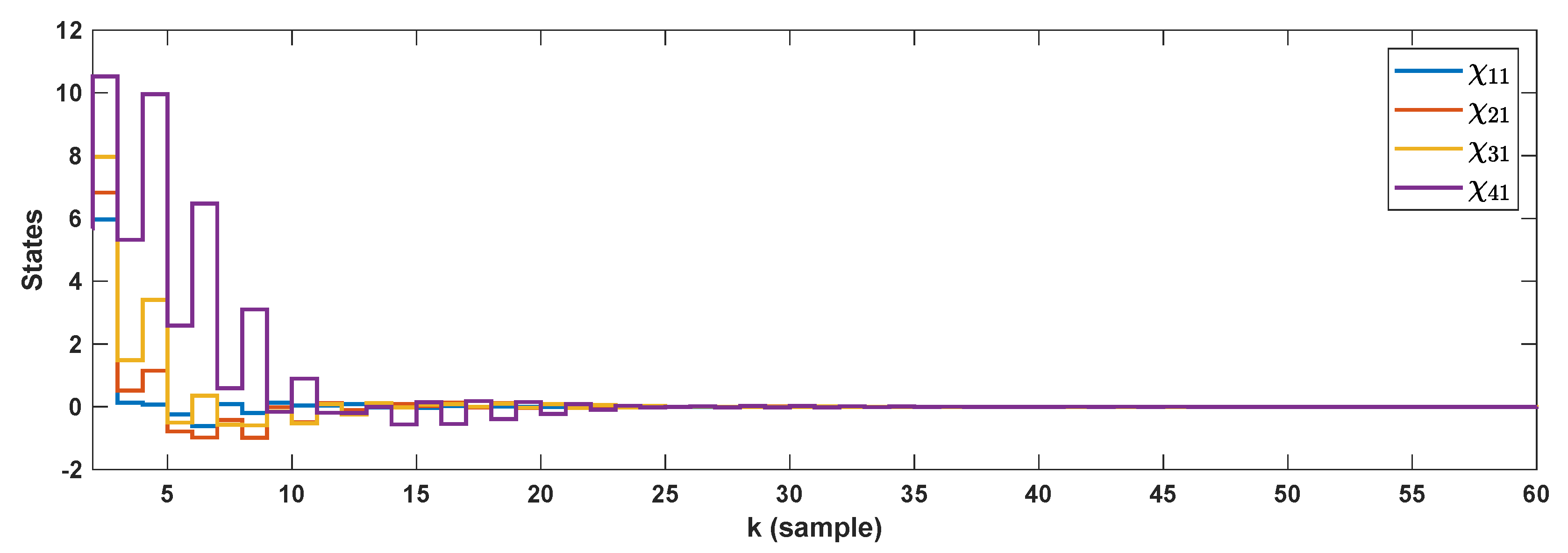
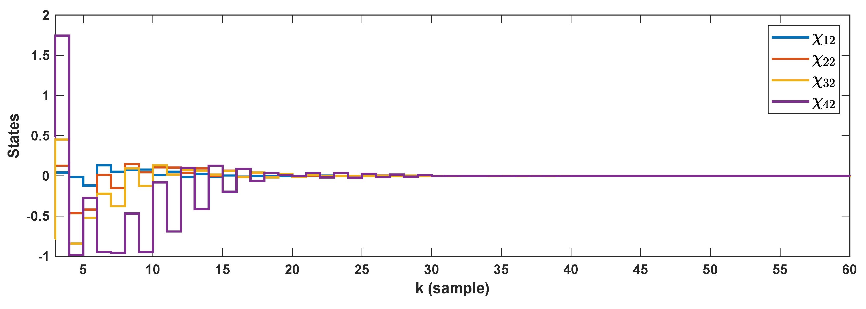
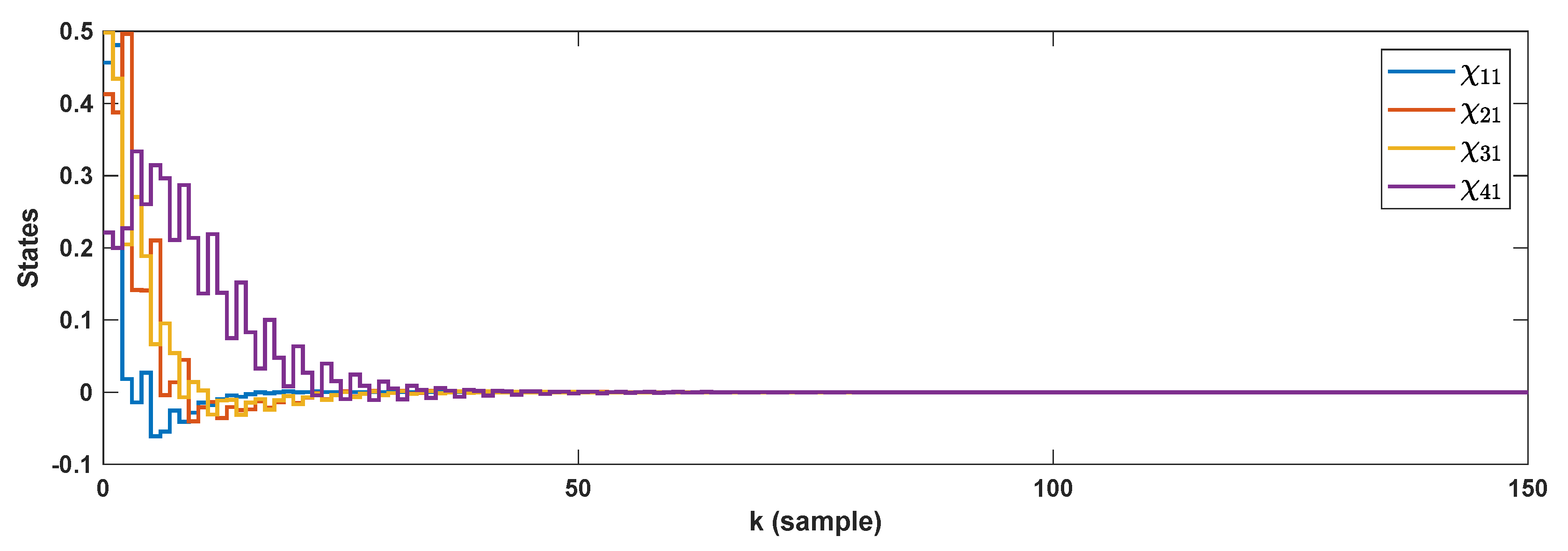
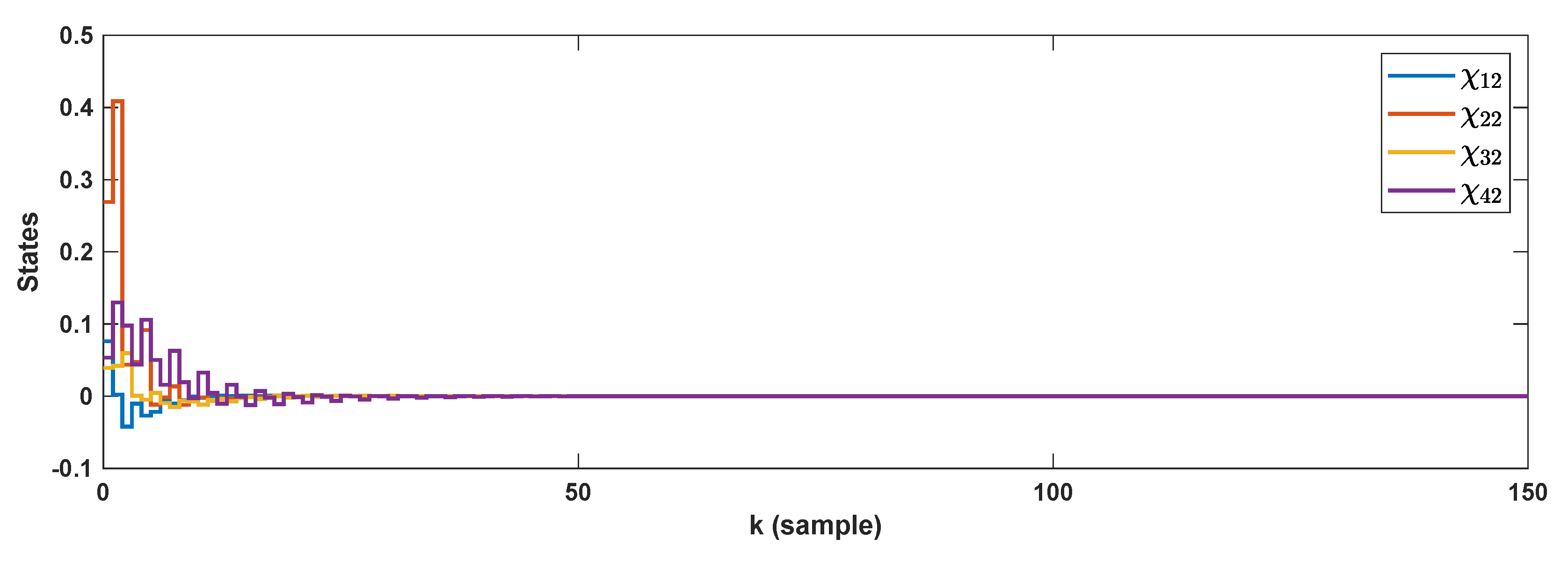
5. Simulation Results

In this section, a Duffing–Holmes chaotic system and a nonlinear heterogeneous MASs are considered to evaluate the effectiveness of the suggested control protocol. Based on the proposed Type-3 fuzzy system and the MPC method, computer simulations are performed and detailed examinations are expressed. Furthermore, the feasibility of the Theorem 1 is analyzed via selecting design parameters.

Example 1.

Consider a network of four agents connected with the following adjacency matrix (the communication topology is portrayed in Figure 4).

$$\begin{array}{c}\hfill \Theta =\left[\begin{array}{cccc}{\theta }_{11}& {\theta }_{12}& {\theta }_{13}& {\theta }_{14}\\ {\theta }_{21}& {\theta }_{22}& {\theta }_{23}& {\theta }_{24}\\ {\theta }_{31}& {\theta }_{32}& {\theta }_{33}& {\theta }_{34}\\ {\theta }_{41}& {\theta }_{42}& {\theta }_{43}& {\theta }_{44}\end{array}\right]=\left[\begin{array}{cccc}0& 1& 1& 0\\ 1& 0& 0& 1\\ 1& 0& 0& 1\\ 0& 1& 1& 0\end{array}\right]\end{array}$$

(48)

The dynamics of agents of the form (1) are considered as a Duffing–Holmes chaotic system:

$$\left\{\begin{array}{c}{\dot{\chi }}_{i_1}={\chi }_{i_2}\hfill \\ {\dot{\chi }}_{i_2}=-\frac{1}{{2.5}^2}{\chi }_{i_1}^3-{\chi }_{i_1}-0.1{\chi }_{i_2}+0.025{\chi }_{i_1}\left(t-\tau \right)\hfill \\ +0.025{\chi }_{i_1}^2\left(t-\tau \right)+0.01{\chi }_{i_2}\left(t-\tau \right)+62.5cos\left(1.29t\right)\hfill \end{array}\right.$$

(49)

It should be noted that the small changes in the initial conditions of chaotic followers lead to severe changes in the dynamic behaviours. The following distributed control policies are applied to the system:

$$\begin{array}{cc}\hfill u_{11}\left(t\right)& ={\widehat{g}}_1^{-1}\left({\chi }_1\left(t\right),{\psi }_{g_1}\left(t\right)\right)\left[-{\widehat{f}}_1\left({\chi }_1\left(t\right),{\psi }_{f_1}\left(t\right)\right)+A_1{\chi }_1\left(t\right)\right]\hfill \\ \hfill u_{12}\left(t\right)& ={\widehat{g}}_2^{-1}\left({\chi }_2\left(t\right),{\psi }_{g_2}\left(t\right)\right)\left[-{\widehat{f}}_2\left({\chi }_2\left(t\right),{\psi }_{f_2}\left(t\right)\right)+A_2{\chi }_2\left(t\right)\right]\hfill \\ \hfill u_{13}\left(t\right)& ={\widehat{g}}_3^{-1}\left({\chi }_3\left(t\right),{\psi }_{g_3}\left(t\right)\right)\left[-{\widehat{f}}_3\left({\chi }_3\left(t\right),{\psi }_{f_3}\left(t\right)\right)+A_3{\chi }_3\left(t\right)\right]\hfill \\ \hfill u_{14}\left(t\right)& ={\widehat{g}}_4^{-1}\left({\chi }_4\left(t\right),{\psi }_{g_4}\left(t\right)\right)\left[-{\widehat{f}}_4\left({\chi }_4\left(t\right),{\psi }_{f_4}\left(t\right)\right)+A_4{\chi }_1\left(t\right)\right]\hfill \end{array}$$

(50)

where ${\widehat{f}}_i$ and ${\widehat{g}}_i$ are T3-FLSs. The FLS parameters are considered in

Table 1. FLS parameters.

${\mathit{C}}_{{\tilde{\mathbf{\Psi }}}_{\mathit{i}}^1},{\mathit{C}}_{{\tilde{\mathbf{\Psi }}}_{\mathit{i}}^2},{\mathit{C}}_{{\tilde{\mathbf{\Psi }}}_{\mathit{i}}^3}$	− 1, 0, 1
${\overline{\Delta }}_{{\tilde{\Psi }}_i^j}$	0.5
${\underline{\Delta }}_{{\tilde{\Psi }}_i^j}$	0.5
$\overline{q}$	0.7, 0.8, 0.9
$\underline{q}$	0.2, 0.3, 0.4
$n_r$	9

.

Moreover, the other control matrices and parameters are selected as:

$$\begin{array}{c}\hfill A_1=\left[\begin{array}{cc}0& 1\\ -{\lambda }_{1,1}& -{\lambda }_{1,2}\end{array}\right],A_{d1}=a_{d1}\times \left[\begin{array}{cc}1& 0\\ 0& 1\end{array}\right]\\ \hfill A_2=\left[\begin{array}{cc}0& 1\\ -{\lambda }_{2,1}& -{\lambda }_{2,2}\end{array}\right],A_{d2}=a_{d2}\times \left[\begin{array}{cc}1& 0\\ 0& 1\end{array}\right]\\ \hfill A_3=\left[\begin{array}{cc}0& 1\\ -{\lambda }_{3,1}& -{\lambda }_{3,2}\end{array}\right],A_{d3}=a_{d3}\times \left[\begin{array}{cc}1& 0\\ 0& 1\end{array}\right]\\ \hfill A_4=\left[\begin{array}{cc}0& 1\\ -{\lambda }_{4,1}& -{\lambda }_{4,2}\end{array}\right],A_{d4}=a_{d4}\times \left[\begin{array}{cc}1& 0\\ 0& 1\end{array}\right]\end{array}$$

(51)

We set the parameters as ${\lambda }_{i,1}={\lambda }_{i,2}=0.10,i=1,2,3,4$, and $a_{d1}=0.2,a_{d2}=0.25,a_{d3}=0.40,a_{d4}=0.60$. Solving the optimization problem of Theorem 1 with the weighting matrices $W_e=\mathrm{diag}\{0.01,0.01\},W_u=0.01$ online leads to $u_{2i}\left(t\right),i=1,\dots ,4$. Then, applying the distributed controller $u_1\left(t\right)=u_{11}\left(t\right)+u_{21}\left(t\right),u_2\left(t\right)=u_{12}\left(t\right)+u_{22}\left(t\right),u_3\left(t\right)=u_{13}\left(t\right)+u_{23}\left(t\right),u_4\left(t\right)=u_{14}\left(t\right)+u_{24}\left(t\right)$, the consensus error dynamics of (35) are stabilized. The state trajectories of the closed-loop MAS and control signals are shown in Figure 5, Figure 6 and Figure 7. We observe a good consensus among agents and appropriate variations for the control trajectories.

For further examination, the effect of time delay is investigated. The delay samples are changed and the values of RMSE are compared. The RMSEs are presented in

Table 2. Effect of time delay.

	Delay Samples
State	1	5	10
${\chi }_{11}$	1.2651	1.2670	1.3021
${\chi }_{12}$	1.0137	1.0172	1.0201
${\chi }_{21}$	1.3560	1.3641	1.3692
${\chi }_{22}$	1.0200	1.0205	1.0212
${\chi }_{31}$	1.5083	1.5302	1.6301
${\chi }_{32}$	1.0290	1.0322	1.0392
${\chi }_{41}$	2.4010	2.4105	2.4532
${\chi }_{42}$	1.0738	1.0802	1.0890

. We can see that the accuracy of the controller does not change in the presence of various time delay samples. Additionally, in

Table 3. Comparison of FLSs.

	FLSs
State	T3-FLS	T2-FLS	T1-FLS
${\chi }_{11}$	1.2651	1.8710	2.0678
${\chi }_{12}$	1.0137	1.9850	2.2001
${\chi }_{21}$	1.3560	1.5101	1.7041
${\chi }_{22}$	1.0200	1.8501	2.0254
${\chi }_{31}$	1.5083	1.5241	1.6950
${\chi }_{32}$	1.0290	1.7014	2.0025
${\chi }_{41}$	2.4010	2.5155	2.6036
${\chi }_{42}$	1.0738	1.7408	1.9052

it is shown that the T3-FLSs result in a lower RMSE. As shown in Table 2 and Table 3, the various time-delays do not affect the accuracy, because the effect of tim -delay as a part of uncertainties is tackled well by the suggested distributed control scheme. It should be noted that at each sample time, the agent dynamics are modeled by the use of T3-FLSs, and then the dynamics uncertainties, as well as the time delays and perturbations, are estimated and tackled by the controller.

Example 2.

To investigate the results of this paper, a nonlinear MAS is considered and we suppose that the communication topology among agents is described by (48).

The dynamics of agents are in the form of (1) with the following parameters:

$$\begin{array}{cc}\hfill {\chi }_1\left(t+1\right)& =f_1\left({\chi }_1\left(t-\tau \right)\right)+g_1\left({\chi }_1\left(t-\tau \right)\right)u_1\left(t\right)\hfill \\ \hfill {\chi }_2\left(t+1\right)& =f_2\left({\chi }_2\left(t-\tau \right)\right)+g_2\left({\chi }_2\left(t-\tau \right)\right)u_2\left(t\right)\hfill \\ \hfill {\chi }_3\left(t+1\right)& =f_3\left({\chi }_3\left(t-\tau \right)\right)+g_3\left({\chi }_3\left(t-\tau \right)\right)u_3\left(t\right)\hfill \\ \hfill {\chi }_4\left(t+1\right)& =f_4\left({\chi }_4\left(t-\tau \right)\right)+g_4\left({\chi }_4\left(t-\tau \right)\right)u_4\left(t\right)\hfill \end{array}$$

(52)

where, $g_i\left({\chi }_i\left(t-\tau \right)\right)=1$ and:

$$\begin{array}{c}\hfill f_1\left({\chi }_1\left(t-\tau \right)\right)={\chi }_3\left(t\right)-3{\chi }_1\left(t\right)+{\chi }_1\left(t\right){\chi }_2(t-\tau )\\ \hfill f_2\left({\chi }_2\left(t-\tau \right)\right)=1-0.1{\chi }_2\left(t\right)-{\chi }_1^2(t-\tau )\\ \hfill f_3\left({\chi }_3\left(t-\tau \right)\right)=-{\chi }_1(t-\tau )-{\chi }_3\left(t\right)\\ \hfill f_4\left({\chi }_4\left(t-\tau \right)\right)=10\left({\chi }_2\left(t\right)-{\chi }_1\left(t\right)\right)\end{array}$$

(53)

We then design the following distributed control policy:

$$\begin{array}{cc}\hfill u_{11}\left(t\right)& ={\widehat{g}}_1^{-1}\left({\chi }_1\left(t\right),{\psi }_{g_1}\left(t\right)\right)\left[-{\widehat{f}}_1\left({\chi }_1\left(t\right),{\psi }_{f_1}\left(t\right)\right)+A_1{\chi }_1\left(t\right)\right]\hfill \\ \hfill u_{12}\left(t\right)& ={\widehat{g}}_2^{-1}\left({\chi }_2\left(t\right),{\psi }_{g_2}\left(t\right)\right)\left[-{\widehat{f}}_2\left({\chi }_2\left(t\right),{\psi }_{f_2}\left(t\right)\right)+A_2{\chi }_2\left(t\right)\right]\hfill \\ \hfill u_{13}\left(t\right)& ={\widehat{g}}_3^{-1}\left({\chi }_3\left(t\right),{\psi }_{g_3}\left(t\right)\right)\left[-{\widehat{f}}_3\left({\chi }_3\left(t\right),{\psi }_{f_3}\left(t\right)\right)+A_3{\chi }_3\left(t\right)\right]\hfill \\ \hfill u_{14}\left(t\right)& ={\widehat{g}}_4^{-1}\left({\chi }_4\left(t\right),{\psi }_{g_4}\left(t\right)\right)\left[-{\widehat{f}}_4\left({\chi }_4\left(t\right),{\psi }_{f_4}\left(t\right)\right)+A_4{\chi }_1\left(t\right)\right]\hfill \end{array}$$

(54)

Let ${\lambda }_{i,1}={\lambda }_{i,2}=0.1,i=1,2,3,4$, and $a_{d1}=0.18,a_{d2}=0.28,a_{d3}=0.38,a_{d4}=0.56$. Based on the optimization problem of Theorem 1 with ${\overline{u}}_2=3$, the distributed control protocols $u_{2i}\left(t\right),i=1,\dots ,4$ are computed. Furthermore, employing the distributed controller $u_1\left(t\right)=u_{11}\left(t\right)+u_{21}\left(t\right),u_2\left(t\right)=u_{12}\left(t\right)+u_{22}\left(t\right),u_3\left(t\right)=u_{13}\left(t\right)+u_{23}\left(t\right),u_4\left(t\right)=u_{14}\left(t\right)+u_{24}\left(t\right)$ online, the consensus error dynamics in the form of (35) are stabilized. The closed-loop system state and applied control trajectories are portrayed in Figure 8, Figure 9 and Figure 10. Similar to Example 1, it can be seen that the consensus among agents is acquired. In addition, it can be seen that the variations in the control protocols are proper.

Remark 1.

The focus of this paper is on designing a distributed control policy in order to achieve a consensus among agents in a finite time. Although optimization-based algorithms have been proposed in [10,32] to analyze the consensus problem of heterogeneous MASs the effects of nonlinear perturbations and unknown time delays have not been considered in these works and only a simple linear dynamical model has been assumed for the agents. This restriction is relaxed in this paper and a wide range of practical systems/implementations can be handled via utilizing the method described in this paper. Note that the suggested control protocol of this paper comprises a learning mechanism that approximates and eases the complexities of the unknown model and uncertainties for designing. This learning mechanism enables the closed-loop system to achieve a consensus when the model is too complex and enhances the convergence rate. Furthermore, the combination of the MPC approach and type-3 FLS results in an optimal hybrid distributed control protocol. It is guaranteed that both approximation and consensus errors are stabilized through the suggested scheme. The results in Figure 5, Figure 6, Figure 7, Figure 8, Figure 9 and Figure 10 verify the usefulness of the policies described in this paper in both aspects of learning an unknown behavior of a system and gaining a consensus among agents for the case of nonlinear systems. Similar results are presented in [10,32]. However, in contrast to the existing results of [10,32], high-order nonlinear terms and unknown dynamical behavior of the system can be tackled by the suggested approach.

6. Conclusions

In this study, a new type-3 fuzzy predictive control scenario is introduced for consensus problems in MASs. Besides the unknown dynamics, some perturbations such as time delay and external disturbances are considered. The suggested predictive scheme improves the consensus accuracy. In two examples, the efficiency is examined. It is shown that the output trajectories of agents are reached the consensus at a finite time. Additionally, the control signal trajectories have appropriate shapes with no fluctuations. In various time delay samples the accuracy is examined, and it is shown that the introduced scenario resists time delays well. Furthermore, a comparison with other FLSs shows that the designed type-3 FLS is more effective. In future works, the optimality of the structure of type-3 FLSs and the effect of actuator faults will be studied.

References

1. Olfati-Saber, R.; Murray, R. Consensus problems in networks of agents with switching topology and time-delays. IEEE Trans. Autom. Control 2004, 49, 1520–1533. [Google Scholar] [CrossRef] [Green Version]
2. Lin, Y.; Lin, Z.; Sun, Z. Distributed Event-Triggered Approach for Multi-Agent Formation Based on Cooperative Localization with Mixed Measurements. Electronics 2021, 10, 2265. [Google Scholar] [CrossRef]
3. Shi, X.; Lin, Z.; Yang, T.; Wang, X. Distributed dynamic event-triggered algorithm with minimum inter-event time for multi-agent convex optimisation. Int. J. Syst. Sci. 2021, 52, 1440–1451. [Google Scholar] [CrossRef]
4. Jin, X.; Lü, S.; Deng, C.; Chadli, M. Distributed adaptive security consensus control for a class of multi-agent systems under network decay and intermittent attacks. Inf. Sci. 2021, 547, 88–102. [Google Scholar] [CrossRef]
5. Nan, X.; Lv, Y.; Duan, Z. On bipartite consensus of linear MASs with input saturation over directed signed graphs: Fully distributed adaptive approach. IET Control Theory Appl. 2021, 15. [Google Scholar] [CrossRef]
6. Shi, X.; Lin, Z.; Zheng, R.; Wang, X. Distributed dynamic event-triggered algorithm with positive minimum inter-event time for convex optimisation problem. Int. J. Control 2020. [Google Scholar] [CrossRef]
7. Seyboth, G.S.; Dimarogonas, D.V.; Johansson, K.H.; Frasca, P.; Allgöwer, F. On robust synchronization of heterogeneous linear multi-agent systems with static couplings. Automatica 2015, 53, 392–399. [Google Scholar] [CrossRef]
8. Jiao, J.; Trentelman, H.L.; Camlibel, M.K. A suboptimality approach to distributed H2 control by dynamic output feedback. Automatica 2020, 121, 109164. [Google Scholar] [CrossRef]
9. Zuo, S.; Lewis, F.L.; Davoudi, A. Resilient Output Containment of Heterogeneous Cooperative and Adversarial Multigroup Systems. IEEE Trans. Autom. Control 2020, 65, 3104–3111. [Google Scholar] [CrossRef]
10. Rahimi, N.; Binazadeh, T. Robust model predictive control of heterogeneous time-delay multi-agent systems with polytopic uncertainties and input amplitude constraints. J. Vib. Control 2021, 27, 1098–1112. [Google Scholar] [CrossRef]
11. Nojavanzadeh, D.; Liu, Z.; Saberi, A.; Stoorvogel, A.A. H and H2 almost output and regulated output synchronization of heterogeneous multi-agent systems: A scale-free protocol design. J. Frankl. Inst. 2021. [Google Scholar] [CrossRef]
12. Liu, Z.; Nojavanzadeh, D.; Saberi, D.; Saberi, A.; Stoorvogel, A.A. Scale-free protocol design for regulated state synchronization of homogeneous multi-agent systems with unknown and non-uniform input delays. Syst. Control Lett. 2021, 152, 104927. [Google Scholar] [CrossRef]
13. Li, K.; Li, Y. Fuzzy adaptive optimal consensus fault-tolerant control for stochastic nonlinear multi-agent systems. IEEE Trans. Fuzzy Syst. 2021. [Google Scholar] [CrossRef]
14. Huang, H.C.; Xu, J.J. Evolutionary Machine Learning for Optimal Polar-Space Fuzzy Control of Cyber-Physical Mecanum Vehicles. Electronics 2020, 9, 1945. [Google Scholar] [CrossRef]
15. Huang, H.C.; Tao, C.W.; Chuang, C.C.; Xu, J.J. FPGA-based mechatronic design and real-time fuzzy control with computational intelligence optimization for Omni-Mecanum-wheeled autonomous vehicles. Electronics 2019, 8, 1328. [Google Scholar] [CrossRef] [Green Version]
16. Huang, H.C.; Chuang, C.C. Artificial Bee Colony Optimization Algorithm Incorporated With Fuzzy Theory for Real-Time Machine Learning Control of Articulated Robotic Manipulators. IEEE Access 2020, 8, 192481–192492. [Google Scholar] [CrossRef]
17. Li, X.; Chen, Y. Discrete Non-iterative Centroid Type-Reduction Algorithms on General Type-2 Fuzzy Logic Systems. Int. J. Fuzzy Syst. 2021, 23, 704–715. [Google Scholar] [CrossRef]
18. Zhang, Z.; Dong, J. Containment control of interval type-2 fuzzy multi-agent systems with multiple intermittent packet dropouts and actuator failure. J. Frankl. Inst. 2020, 357, 6096–6120. [Google Scholar] [CrossRef]
19. Mohammadzadeh, A.; Zhang, W. Dynamic programming strategy based on a type-2 fuzzy wavelet neural network. Nonlinear Dyn. 2019, 95, 1661–1672. [Google Scholar] [CrossRef]
20. Valdez, F.; Castillo, O.; Cortes-Antonio, P.; Melin, P. A survey of Type-2 fuzzy logic controller design using nature inspired optimization. J. Intell. Fuzzy Syst. 2020, 39, 6169–6179. [Google Scholar] [CrossRef]
21. Chen, C.H.; Jeng, S.Y.; Lin, C.J. Mobile robot wall-following control using fuzzy logic controller with improved differential search and reinforcement learning. Mathematics 2020, 8, 1254. [Google Scholar] [CrossRef]
22. Lee, C.L.; Lin, C.J. Integrated computer vision and type-2 fuzzy CMAC model for classifying pilling of knitted fabric. Electronics 2018, 7, 367. [Google Scholar] [CrossRef] [Green Version]
23. Qasem, S.N.; Ahmadian, A.; Mohammadzadeh, A.; Rathinasamy, S.; Pahlevanzadeh, B. A type-3 logic fuzzy system: Optimized by a correntropy based Kalman filter with adaptive fuzzy kernel size. Inf. Sci. 2021, 572, 424–443. [Google Scholar] [CrossRef]
24. Chen, C.; Lewis, F.L.; Xie, K.; Xie, S.; Liu, Y. Off-policy learning for adaptive optimal output synchronization of heterogeneous multi-agent systems. Automatica 2020, 119, 109081. [Google Scholar] [CrossRef]
25. Jiang, Y.; Fan, J.; Gao, W.; Chai, T.; Lewis, F.L. Cooperative adaptive optimal output regulation of nonlinear discrete-time multi-agent systems. Automatica 2020, 121, 109149. [Google Scholar] [CrossRef]
26. Mohammadzadeh, A.; Kaynak, O. A novel general type-2 fuzzy controller for fractional-order multi-agent systems under unknown time-varying topology. J. Frankl. Inst. 2019, 356, 5151–5171. [Google Scholar] [CrossRef]
27. Li, S.; Er, M.J.; Zhang, J. Distributed Adaptive Fuzzy Control for Output Consensus of Heterogeneous Stochastic Nonlinear Multiagent Systems. IEEE Trans. Fuzzy Syst. 2018, 26, 1138–1152. [Google Scholar] [CrossRef]
28. Chen, C.L.P.; Ren, C.E.; Du, T. Fuzzy Observed-Based Adaptive Consensus Tracking Control for Second-Order Multiagent Systems With Heterogeneous Nonlinear Dynamics. IEEE Trans. Fuzzy Syst. 2016, 24, 906–915. [Google Scholar] [CrossRef]
29. Zou, W.; Ahn, C.K.; Xiang, Z. Fuzzy-Approximation-Based Distributed Fault-Tolerant Consensus for Heterogeneous Switched Nonlinear Multiagent Systems. IEEE Trans. Fuzzy Syst. 2021, 29, 2916–2925. [Google Scholar] [CrossRef]
30. Yang, Y.; Xu, C.Z. Adaptive Fuzzy Leader-Follower Synchronization of Constrained Heterogeneous Multiagent Systems. IEEE Trans. Fuzzy Syst. 2020. [Google Scholar] [CrossRef]
31. Shi, P.; Yu, J. Dissipativity-Based Consensus for Fuzzy Multiagent Systems Under Switching Directed Topologies. IEEE Trans. Fuzzy Syst. 2021, 29, 1143–1151. [Google Scholar] [CrossRef]
32. Jiao, J.; Trentelman, H.L.; Camlibel, M.K. H2 suboptimal output synchronization of heterogeneous multi-agent systems. Syst. Control Lett. 2021, 149, 104872. [Google Scholar] [CrossRef]
Figure 1. The general scheme of the controller.
Electronics 11 00063 g001
Figure 2. General identification and learning structure.
Electronics 11 00063 g002
Figure 3. Type-3 FS.
Electronics 11 00063 g003
Figure 4. Topology.
Electronics 11 00063 g004
Figure 5. Example 1: First state trajectories.
Electronics 11 00063 g005
Figure 6. Example 1: Second state trajectories.
Electronics 11 00063 g006
Figure 7. Example 1: Control signals.
Electronics 11 00063 g007
Figure 8. Example 2: First state trajectories.
Electronics 11 00063 g008
Figure 9. Example 2: Second state trajectories.
Electronics 11 00063 g009
Figure 10. Example 2: Control signals.
Electronics 11 00063 g010