A Novel Hybrid Approach Based on Deep CNN to Detect Glaucoma Using Fundus Imaging

Abstract

Glaucoma is one of the eye diseases stimulated by the fluid pressure that increases in the eyes, damaging the optic nerves and causing partial or complete vision loss. As Glaucoma appears in later stages and it is a slow disease, detailed screening and detection of the retinal images is required to avoid vision forfeiture. This study aims to detect glaucoma at early stages with the help of deep learning-based feature extraction. Retinal fundus images are utilized for the training and testing of our proposed model. In the first step, images are pre-processed, before the region of interest (ROI) is extracted employing segmentation. Then, features of the optic disc (OD) are extracted from the images containing optic cup (OC) utilizing the hybrid features descriptors, i.e., convolutional neural network (CNN), local binary patterns (LBP), histogram of oriented gradients (HOG), and speeded up robust features (SURF). Moreover, low-level features are extracted using HOG, whereas texture features are extracted using the LBP and SURF descriptors. Furthermore, high-level features are computed using CNN. Additionally, we have employed a feature selection and ranking technique, i.e., the MR-MR method, to select the most representative features. In the end, multi-class classifiers, i.e., support vector machine (SVM), random forest (RF), and K-nearest neighbor (KNN), are employed for the classification of fundus images as healthy or diseased. To assess the performance of the proposed system, various experiments have been performed using combinations of the aforementioned algorithms that show the proposed model based on the RF algorithm with HOG, CNN, LBP, and SURF feature descriptors, providing ≤99% accuracy on benchmark datasets and 98.8% on k-fold cross-validation for the early detection of glaucoma.

1. Introduction

Medical research is playing a vital role to protect people from the long-lasting effects of various diseases. Moreover, the eye is the most important visual organ. The detection of eye diseases is performed by the experts based on manual methods, such as analyzing the images of the defective eyes. Based on these examinations, the disease is treated by taking various measures to prevent the infection of this disease and its growth. However, these methods are expensive, time-consuming, and less accurate. To avoid such problems, computer-aided techniques are used, which assist the experts to diagnose and treat such diseases within the least time and with better accuracy. Among various eye diseases, glaucoma is also one of the most fatal diseases. During this disease, a person’s ocular nerves are damaged, due to which eyesight can be lost, and this loss is irreversible. The causes of this disease remains unrevealed. However, intraocular pressure, heredity, and high myopia cause the progression of disease. This disease has no symptoms until it reaches the advanced stage. Therefore, to avoid such disease, proper care must be taken to diagnose and treat this disease at an early stage.

As the population is increasing day by day, patients with glaucoma are also increasing rapidly due to diabetes. Diabetic patients are at higher risk of developing diabetic retinopathy which have some common risk factors with glaucoma such as ganglion cell loss, and elevated oxidative stress etc. [1]. Therefore, the patients with diabetes may experience the symptoms of glaucoma. Glaucoma was declared the other major reason of blindness all over the world as estimated by the World Health Organization (WHO). Retinal or fundus images are the source of detection of disease in the eyes. Glaucoma is also diagnosed from the fundus images. The key factor to cause glaucoma is a disproportion in the volume of fluid that maintains the eye shape. This produces pressure on the optic nerve head (ONH) and causes damage. The images scanned from the vision are converted into visual signals and sent to the brain using retinal nerves on the optical disc (OD). The OD consists of photoreceptors, i.e., rods and cones, that support vision. Moreover, 30% of the brightest regions exist on the OD, i.e., optic cup (OC), in a healthy eye. Various medical methods have been used for the detection of glaucoma such as fundus images [2], optical coherence tomography (OCT) [3], and analysis of lateral geniculate nucleus in glaucoma patients through magnetic resonance imaging (MRI) [4], etc. In this study, fundus images will be used that will be captured from the fundus camera. The fundus cameras capture a clear and in-depth view of the retina, giving the practitioners a detailed analysis. It has the characteristic of changing filters to enhance the fundus images captured at different angles.

In the fundus images, the prominent portion on the retina is the OD that consists of an OC and neuro-retinal rim. Glaucoma can be detected easily as the size of OC increases. Therefore, in this study, we will use five stages, namely pre-processing, segmentation, feature extraction, feature selection and ranking, and classification. In pre-processing, fundus images will be improved by removing noise and outliers. Features are extracted with the help of combinations of convolutional neural networks (CNN) with a HOG, LBP, and SURF. Furthermore, the MR-MR method based on ranking is employed for feature selection. For the classification, three different algorithms have been applied, i.e., SVM, KNN, and RF.

The remaining paper has been organized as follows. Section 1 presents the Introduction, while Section 2 refers to the existing work performed concerning glaucoma detection. Section 3 presents the proposed system, and Section 4 and Section 5 report the performed experiments and present the conclusion.

2. Related Work

In glaucoma disease, the optic disc enlarges from the original size due to abnormal conditions in the eye. The signals generated from the vision transmit to the brain through optic nerves. The regions of nerves that have no rods and cones are called blind spots. In a healthy eye, the OD diameter is around 1.5 mm [5]. Various segmentation techniques have been applied for the detection of OD, as it is brighter than other parts of the retina [6,7]. Segmentation is the process to extract the foreground image as a region of interest and separate it from the background. In [8], a segmentation-based technique has been proposed based on the fuzzy C-means clustering algorithm. The weighted distance has been computed between pixel and center point. In the end, the fuzzy coefficient is computed and the algorithm outperforms some of the existing segmentation algorithms. Another segmentation-based technique, namely one-pass aligned atlas set for images segmentation (OASIS), has been proposed for MR images [9]. For the segmentation of OD, the template-based technique is proposed [10]. Watershed transform algorithms are employed on a modified variance image. The algorithm obtained 90% accuracy. Furthermore, canny edge detection and Hough transformation have been used for the localization of OD [11]. The performance evaluation depicts that the proposed work attained 97% accuracy for localization and 82% accuracy for the segmentation. Liu et al. [12] employed a technique based upon the morphology and gradient vector to detect the OD using localization and segmentation. The accuracy is 96.7% and sensitivity is 95.1%. Intensity-based feature extraction has been used to extract multi-features [13], and a deep learning-based model was adopted to classify the images using standard datasets [14,15]. OC-based segmentation is a challenging task to detect glaucoma. The variation level-based method has been used for the segmentation of the OC [16]. The edges in the polar regions have been detected for the detection of glaucoma. This technique is based upon the ARGALI, an automated system that employs numerous methods for the OD and OC segmentation. The segmentation of OC is performed using a fixed thresholding technique [17]. Cheng et al. employed super pixel-based segmentation of OC [18], which considers the medium-sized OC.

Another important field of glaucoma research is based on deep learning algorithms. Convolutional neural networks architectures have been employed on the fundus images to detect glaucoma [19,20,21,22,23,24]. A fully convolutional neural network has been employed for the training and classification of OC and DC simultaneously [25]. Entropy sampling has been used for the segmentation of OC and OD [26]. Path classification is employed with the help of a deep learning model for the detection of a defect in retinal nerves [27]. Local features and holistic features with a combination of deep convolutional networks have been used for the classification of glaucoma [20]. A deep residual algorithm has been employed on the fundus images for the detection of glaucoma and the results have been compared with ophthalmologists [28]. The sparse auto-encoder-based technique is used for the detection of glaucoma [29]. Various techniques have been used for the detection of glaucoma, however most require more time for detection and classification and achieve less accuracy than our proposed model. A summary of the state-of-the-art techniques is reported in

Table 1. Summary of the existing Techniques for Glaucoma Detection.

Reference	Task Type	Datasets	Results	Remarks
[24]	Classification	ORIGA and SCES	83% and 88%	Fundus images are classified into two classes using CNN having overlapping pooling layers
[30]	Classification	499 Images of Patients	97%	Decision trees, SVM, KNN, and RF are compared for different eye measurement images.
[31]	Classification	279 Images	92%	Feedforward neural networks are used on visual fields for the detection of pre-parametric glaucoma
[32]	Classification	48,116 Fundus Images	98%	Fundus images being classified into glaucoma certain and glaucoma suspected
[26]	OC and OD Segmentation	RIM-ONE, Messidor, DRISHTI-GS	80%, and IOU: disc 89%	Key points selection is done based on entropy sampling using convolutional filters
[33]	OD and Vessels Segmentation	DRIONS-DB, RIM-ONE	95% precision and 95% recall	A pre-trained VGG neural network with full convolutional layers is used and various internal layers are supervised
[34]	Disc, vessels and fovea Segmentation	DRIVE	IOU: 62%	33 × 33 central pixels patch is classified using 7 layered CNN into vessels, fovea, disc and background
[35]	Disc Segmentation	SiMES	IOU: 90%	Handcrafted features are used for the pixel-wise segmentation and 7 layered CNN is used separately to test the segmentation of OD
[36]	Classification	28 fundus images	Not Reported	Texture features are extracted from nerve fibers layers
[37]	Not Reported	71 fundus images	97.2%	Optic Cup detection using Neuro Retinal Images
[38]	Not Reported	1866 images	Not Reported	Retcam images are used with close angle for Glaucoma Detection
[39]	Classification	60 fundus images	91%	High order spectra features and texture images are used for glaucoma detection

.

The main contributions of the proposed work are below:

• A novel and robust algorithm has been proposed that can perform the early detection of eye disease, i.e., glaucoma in the fundus images exhibiting retina. The hybrid feature descriptors are employed to extract features, such as CNN with LBP, HOG, and SURF. Moreover, a feature selection algorithm, i.e., MR-MR, has been used to select the most representative features for the classification. In the end, binary classifiers have been used for the detection of diseases, such as KNN, RF, and SVM.
• The proposed technique is novel for the detection of glaucoma. It uses a region of interest based on a template that ensures the extraction of a defective part in the fundus image of the retina. Furthermore, it has been proven that the presence of pathological structures, blood vessels, noise, irregular shapes of OD, and un-even brightness affects the segmentation of OD. However, the proposed technique performs effectively in the above scenarios.
• The performance of the proposed algorithm is evaluated on a 40% testing dataset (1500 Fundus Images). In addition, k-fold cross-validation for k = {1, 2, 3, 4, 5} is performed using two datasets, i.e., DRISHTI-GS and RIM-ONE. The algorithm obtained 99% on testing images and 98.8% accuracy on cross-validation.

3. Proposed Methodology

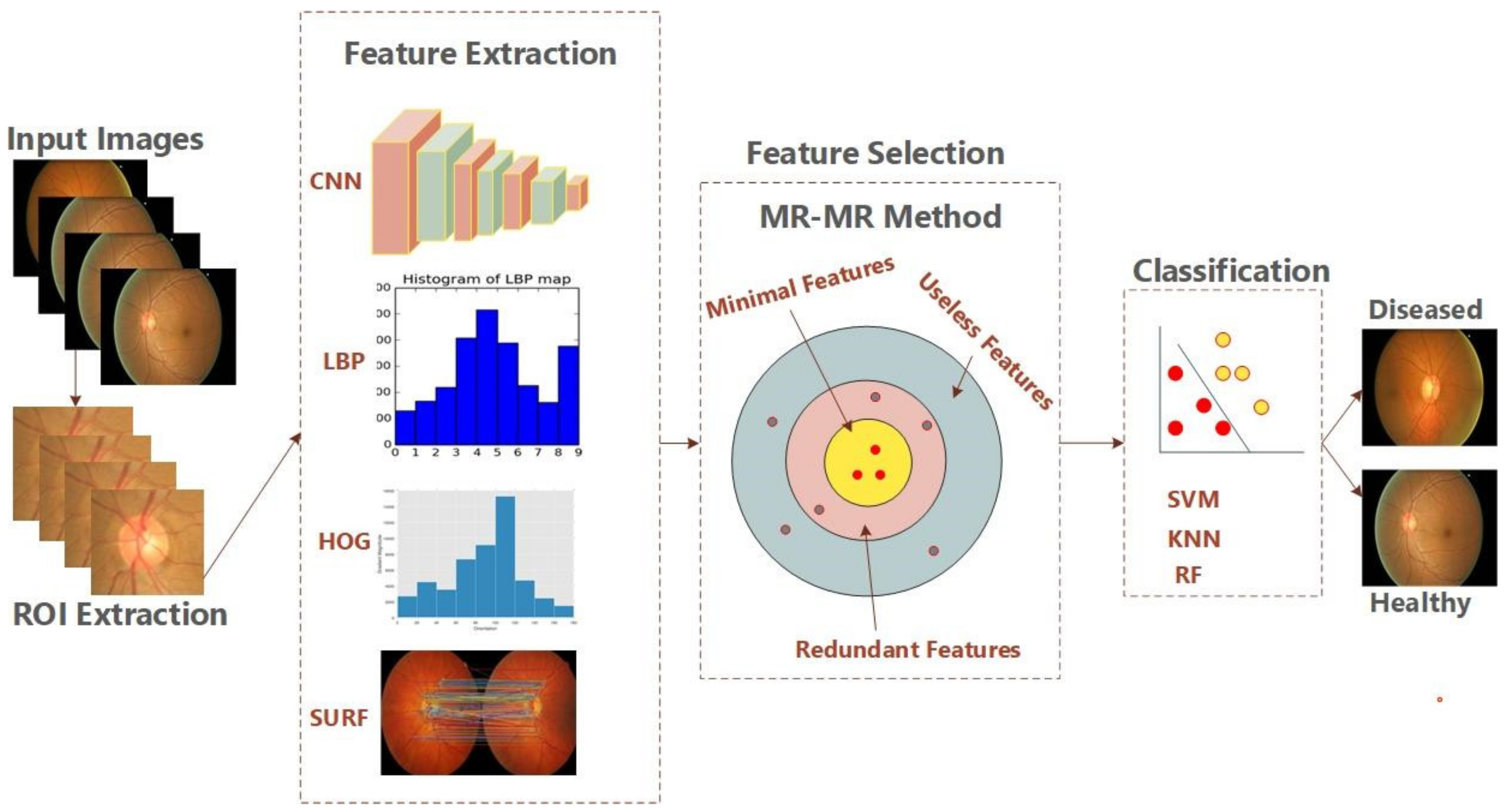
Because retinal disease is such a serious condition, detecting and recognizing it is a difficult challenge in medicine. There are a variety of image processing models for detecting retinal illness. However, the results aren’t always accurate. The suggested system’s first phase is pre-processing, which involves detecting and removing noise from images. Then, to identify the unique properties from images, ROI is identified, and segmentation is performed. Furthermore, deep convolutional neural network (DCNN) hybridizes as CNN with HOG, LBP, and SURF, and a combination of all of them in the third stage to extract the features from ROI. The features used for detection and classification are texture, contrast, scaling, rotation, and translation. In the next step, a method for the most representative features selection has been employed to remove irrelevant features. Furthermore, to categorize the images into two classes, diseased and healthy, these computed features are fed to multiclass classifiers, i.e., SVM, KNN, and RF. Figure 1 shows some sample photos for each class. The following is a breakdown of the suggested deep learning-based model.

3.1. Pre-Processing

In the first phase, the images need to be pre-processed first to use them in the system’s next steps. This phase involves format conversion while also boosting image quality. The TIFF format is used to convert images since it keeps the original properties of the images without information loss. Finally, images have been downscaled from all dimensions using a bilinear technique to reduce computing complexity. This also reduces noise because, unlike the bilinear technique, the pixel’s output value is computed as the average of the pixel’s weights in 2 × 2 neighbors. Fundus samples are shown with preprocessing results in Figure 2.

3.2. Segmentation

Thus, OC present in the eyes has main features that exhibit the glaucoma disease. The OC size increases as the disease advances. Thus, the ROI for the detection of glaucoma is OD that consists of OC. The ROI is computed using an identical method with the record of fundus images. The record image travels over each pixel of the image and the resemblance between the sample’s blocks using HOG features is calculated. The portion exhibiting maximum resemblance is chosen as the ROI. This proposed technique for ROI identification outperforms the existing algorithms. Suppose I is the input image that needs to be pre-processed with size I × J, and D is the record of images with size of dr × dc. Suppose vd represents the vector of HOG with a size of 1 × h of the record D. Let sm,n represent the portion situated in the image I (m,n) as dr × dc. The features determined by HOG are referred to as ${℣}_{m,n}^s$. Mean absolute difference (MAD) has been employed to calculate the resemblance among the record of images D and the image block sm,n.

$${ῡ}_{m,n}=\frac{1}{h}{\displaystyle \sum }_{l=1}^h \left[{℣}_{m,n}^s \left(l\right)-{℣}^d\right]$$

(1)

The chunk having minimum MAD has been assigned as ROI which consists of the OD. The carefully chosen region has important features as it has the OD having OC.

Segmentation: After mining of ROI, this extracted image is fed to employ the segmentation using the active contour algorithm. The ROI has been segmented, now employing 3 × 3 masks.

3.3. Deep Learning

Deep Learning uses a hierarchical approach to accomplish nonlinear transformations. The convolutional neural network (CNN) features based on deep design with a feed-forward topology make learning simple. CNN’s layers can analyze the features deeply and show a lot of variation. Through the testing step of the DCNN, all layers are differentiated and run in the forward direction. Deep CNN’s key feature is that it searches for every possible match between samples. Convolutional layers linearize the manifold, whereas pooling layers make it compact. The size of the layer at the output is determined by the stride. Suppose the size of the kernel is K × K and the size of input is S × S, and the 1 is the size of stride. The input feature maps are F and for output O. Hence, the size of input is FҨ S × S, the size of output is O Ҩ (S−K+1) × (S−K+1), the kernel consists of the F × O × K × K factors that are needed to be taught, and the required cost is F × K × K × O × (S−K+1) × (S−K+1). The size of the filter needs to be harmonized with the output size pattern that needs to be recognized. The output size is dependent upon the stride among the pools, e.g., if independent pools have the size K × K and size of input is S × S having features F, then the output becomes as F Ҩ (S/K) × (S/K).

The output function can be written mathematically as below:

$$\mathrm{F}=\mathrm{FL} o \mathrm{FL}-1 o ..........\mathrm{F}1$$

(2)

where $\mathrm{F}\mathrm{L}$ represents the layer that takes the previous’ layer output as xL−1 to compute the output xL considering the weights $\omega$L for each layer, as shown below:

$$x\mathrm{L}= \mathrm{FL}\left(x\mathrm{L}-1; \omega \mathrm{L}\right) for \mathrm{L}=2,3,....l$$

(3)

3.4. Feature Extraction

The form of the OC is used to extract features, which is dependent on its size. Area, density, edge, distances (maximum and minimum axial distances), rotation, width, and convex area are among the retrieved level characteristics. HOG is used to calculate low-level features, whereas the LBP descriptor is used to compute texture features. ConvNet, on the other hand, is used to calculate high-level features, like scaling, translation, and rotation. Distinct feature descriptors are employed in current methods. However, they have failed to correctly diagnose glaucoma illness. High- and low-level features have been employed in our proposed approach to produce features of fundus images that outperform the existing techniques of feature extraction.

3.4.1. CNN as Feature Descriptor

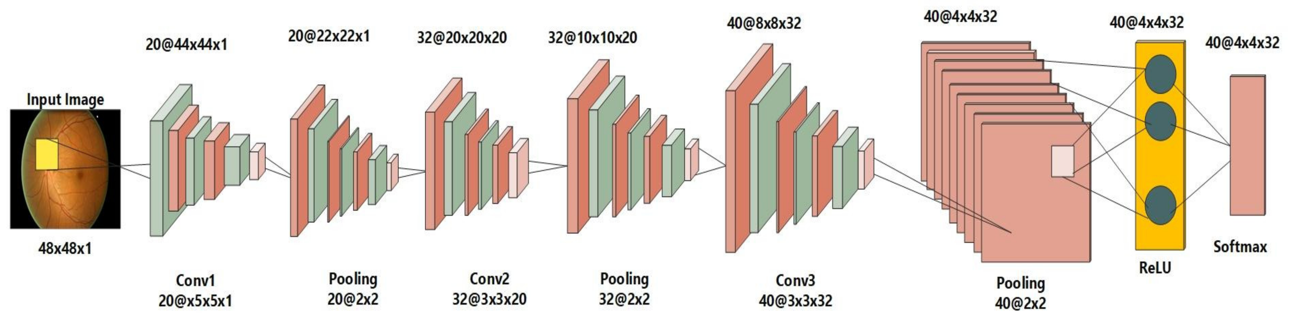
The network’s 1st layer is a convolutional layer of our proposed 2-D CNN that has a filter size 20 and a size of stride 1. The next layer is the pooling layer, which is 2 × 2 with a stride of 1. The following layer is another convolutional layer having filter size 32 and stride of 1. These both layers alternately make up the first six layers. The activation layer is the seventh layer, using a rectified linear unit (ReLU), whereas the convolutional layer is the 8th one, having a filter size of 40. (4 × 4 × 32). A softmax function layer is the last layer. For useful calculations, the weights of convolutions and the variable values in max-pooling layers should remain constant. The image size in our sets is 50 × 50 × 1, which is converted to 1 × 1 × 2 via forwarding propagation of all layers. Figure 3 depicts the Deep Neural Network layers utilized in the suggested approach. Convolutional layers in CNN take image I as input and apply filters f with size of m x n, length l, bias b, and weights w. As a result, the output may be expressed as an equation as follows:

$$\left(I*f\right)x,y={\displaystyle \sum }_{s=1}^l {\displaystyle \sum }_{t=1}^w fst.I_{x+s-1,y+t-1}+b$$

(4)

3.4.2. HOG as Feature Descriptor

As images are transformed into contiguous blocks ranging in size from 28 × 28 to 6 × 6, with each block measuring 2 × 2 and a stride of 4. There are a total of 9 bins created. There are a total of 1296 low-level attributes calculated. At this point, normalization can be used to improve feature extraction. Normalization improves the intensity and shadow of pulmonary images. Intensity is considered in the larger image size block. Since the opposing orientations of the image portion are placed in the same bin, a similar orientation is computed for them. The angle’s range remains 0–180 degrees. The pixel (x, y gradient)’s magnitude M and direction are provided in the equation below:

$$M \left(x,y\right)=\sqrt[2]{I{x}^2+I{y}^2}$$

(5)

The direction of the pixel is calculated as below:

$$\vartheta ={\tan }^{-1}\frac{I_y}{I_x}$$

(6)

Here, the angle $\vartheta$ changes from 0 to 2Л, whereas $I_y$ and $I_x$ represent the gradients in x and y directions.

3.4.3. LBP as Feature Descriptor

The LBP is employed to extract texture-based characteristics and operates on the concept that each pixel matches itself to its neighbor’s and, consequently, uses the threshold function to encode the local neighbor’s [40]. If the neighbors’ grey values are higher than or equal to the center pixels, then its value is set to 1. LBP creates its dual feature vectors, e.g., 2k, by letting K indicate the total number of adjacent pixels. As a result, there will be 65,536 feature vectors for 16 pixels, with the number increasing with the surrounding pixels’ sizes. The LBP’s mathematical equation is presented below.

$$LBP={\displaystyle \sum }_{i=0}^{1}k\left(p-c\right){.2}^i,$$

(7)

$$k\left(x\right)=\left\{\begin{array}{c}1\\ 0\end{array}\right.\begin{array}{c} if x\ge 0\\ otherwise\end{array}$$

(8)

where p refers to the adjacent pixel and c represents the middle one.

3.4.4. SURF as Feature Descriptor

SURF [40] as a feature descriptor is an efficient method that extracts the most representative features for the object detection and classification. The main steps of the method include the selection of key points, extraction of the descriptors, and matching of the descriptors among various images. For the first step, the images are filtered employing box filters. The time for the filtering process is minimized using an integral image computing the pixel value from the original image by adding the above and left side pixels. Then, the Hessian matrix is formed to find the key points after convolution over box filters. Those points have been selected where the determinant of the Hessian matrix is highest. Suppose the image I has a point as s = (i,j) and Hessian matrix is H(s,𝜎), where s is scale and 𝜎 is given in Equation (9). The original image size remained the same whereas scaling is applied employing different filter sizes (usually up scaling the size). The scale can be computed as described in Equation (10).

$${\sigma }_{appr}=present\_Filte{r}_{size} x \left(\frac{Initial\_FIlter\_Scale}{Initial\_Filter\_Size}\right)$$

(9)

$$H\left(s,\sigma \right)=\left[\begin{array}{cc}{K}_{pp}\left(s,\sigma \right)& K_{pq}\left(s,\sigma \right)\\ K_{pq}\left(s,\sigma \right)& K_{qq}\left(s,\sigma \right)\end{array}\right]$$

(10)

Here, $K_{pp}\left(s,\sigma \right)$ refers to the convolved output of the image at s along with the 2nd order derivation of Gaussian box filter. Similarly, the remaining components have been computed. The Hessian matrix determinant is represented in Equation (11).

$$\det \left(H\right)=K_{pp}\left(s,\sigma \right) x K_{qq}\left(s,\sigma \right)-K_{pq}\left(s,\sigma \right)$$

(11)

After the computation of the determinant, we want to select the reproducible orientation of selected key points. Therefore, we achieved this using information mining from the region surrounding the required points. Moreover, a square region is formed that is aligned to the selected orientation and then the features have been extracted from the key points. The Laplacian sign indexing technique has been utilized for feature matching. It identifies the prominent blobs in images having dark backgrounds. The matching is performed on those features which have the same contrast level, consequently improving the performance of the method. The SURF descriptor extracts the features based on brightness invariance, translation invariance, rotation, and scale invariance.

3.5. Feature Selection and Ranking

MR-MR [41] is the method of feature selection, i.e., to find the most representative features for the objective class when the extracted features become less redundant. In our proposed method, the objective classes are two, i.e., diseased and healthy. Thus, to select most representative features, it is necessary to improve the information among the objective class and features. Suppose i and j are points, the combined information between i and j is represented as Ώ in Equation (12). The combined information represents the highest dependency among the i and j.

$$\mathsf{Ώ}\left(i,j\right)={\iint }_{ }^{ }p\left(i,j\right)log\frac{p\left(i,j\right)}{p\left(i\right). p\left(j\right)} di ds$$

(12)

Suppose, R(S,j) represents the combined information among a feature set as S = {m₁,m₂,….,m_n} and target class j. Therefore, the combined information is described in Equation (13).

$$\left[R\left(S,j\right)\right]=\frac{1}{\left|S\right|}{\displaystyle \sum }_{m_iϵS} \mu \left(m_i,j\right)$$

(13)

The selected features have a maximum relevance that causes the maximum redundancy. Therefore, to minimize the redundancy, Equation (14) is presented. Suppose, D(S) refers to the combined information among two features m_i and m_k in set S.

$$\left[D\left(S\right)\right]=\frac{1}{{\left|M\right|}^2}{\displaystyle \sum }_{m_i,m_k\in S} \mu \left(m_i,m_k\right)$$

(14)

The combination of the Equations (13) and (14) is called the MR-MR method. The method searches for the compact set of features having maximum relevance and minimum redundancy by increasing the R(S,j) and decreasing D(S). The combined objective function is represented as ꞕ(R,D) and defined in Equation (15).

$$max\left[ꞕ\left(R,D\right), ꞕ\right]=R-D ,$$

(15)

The most representative optimal features that can be represented by ꞕ(..) can be found employing incremental search techniques [41].

3.6. Classification

After the feature extraction and selection phase, the most important step is to classify the selected features. For the detection of glaucoma, selected features have been passed to our trained classifiers for the categorization of images into diseased and healthy images based on the ROI. The ROI for the detection of glaucoma is an enlarged optic disc (OD) comprising of optic cup (OC). For the training of the classifiers, we have employed train and test sets of fundus images split as 60% and 40% respectively. Therefore, to choose the best algorithm, we employed three machine learning based methods to classify the data. SVM is a supervised learning method which is taught using extracted features in two classes: healthy and unhealthy. One of the memory-efficient approaches is SVM. The random forest (RF) algorithm, which uses several de-correlated decision trees and is excellent over huge datasets, is therefore used. In addition, the KNN, which is the simplest of all, is employed. It uses a voting method to classify the data and identifies undefined data. If k is 1, the present object is assigned to the closest neighbor class in KNN. The suggested system’s algorithm is shown in Algorithm 1. The proposed architecture is shown in Figure 4.

Algorithm 1: Pseudocode for the proposed System.

Input: $Images=\left\{I_1,I_2,I_3,\dots \dots \dots ..I_k\right\}$

Output: $Classified Images$

Start:

record(i) ← 1….k

While(record(i)!= eof){

Perform Pre-processing over the images Ik

CNNF ← 2DCNN Perform Feature Computation

HOGF ← Feature Computation using HOG

LBPF ← Feature Extraction using LBP

SURF ← Feature Extraction using SURF

Fea_Vec ← (CNN, LBP, HOG, SURF)

Fea_Comb ← (CNN with HOG, SURF, CNN with HOG and LBP, CNN with LBP, HOG, and SURF)

Selected ← MR-MR()

Labels ← Annotations (Diseased, Healthy)

Class ← (SVM (Selected, CL, testSet) KNN (Selected, CL, testSet) RF (Selected, CL, testSet))

j = 1;

While (j≤n)

{

IF(Class(j)) ← Diseased

{Output “Glaucoma Detected”

ELSE IF(Class(j)) ← Healthy

Output “Healthy Eye”

}

END

4. Experimental Evaluation

In this section, we report the experiments and results attained using the said datasets. The efficacy of the proposed method was verified on a huge dataset and the results were computed using various metrics. Moreover, other than training and testing, cross-validation is executed to evaluate the robustness of our proposed system. Furthermore, a state-of-the-art comparative investigation is accomplished. Therefore, in the reported outcomes, it is shown that our proposed model outperforms the existing segmentation-based techniques for the detection of glaucoma eye disease.

During the training phase, features have been extracted using a combination of CNN with HOG, LBP, and SURF, respectively. In CNN, the total number of convolutional layers was 20 and the pooling layer’s size was 2. Moreover, both types of layers were alternatively present three times in a network. The ReLU layer was employed for the activation. For the classification purpose, the Softmax function was utilized at the final layer. In 1900 iterations, the average accuracy was 97%. We employed three classification algorithms, i.e., SVM, KNN, and RF, to classify the images into two classes, i.e., healthy, and unhealthy. Initially, an SVM algorithm was employed and trained over samples of positive and negative classes. Then, KNN and RF are trained for all combinations of feature descriptors. The training time is reported in

Table 2. Training Time for the Proposed Algorithms.

Classifier Name	Time in Seconds
SVM + LBP	5.2 s
SVM + HOG	4.1 s
SVM + CNN	2.81 s
SVM + SURF	3.7 s
SVM + HOG + CNN	3.8 s
SVM + CNN + LBP	3.18 s
SVM + CNN + SURF	3.9 s
SVM + HOG + CNN + LBP	9.5 s
SVM + HOG + CNN + LBP + SURF	11 s
RF + HOG	4.5 s
RF + CNN	4.2 s
RF + SURF	2.5 s
RF + LBP	2.4 s
RF + CNN + LBP	2.8 s
RF + CNN + SURF	3.1 s
RF + HOG + CNN + LBP	8.9 s
RF + HOG + CNN + LBP + SURF	9.0 s
RF + HOG + CNN	7.8 s
KNN + HOG	3.6 s
KNN + CNN	4.3 s
KNN + LBP	2.3 s
KNN + SURF	4.2 s
KNN + CNN + HOG	6.8 s
KNN + HOG + CNN	2.7 s
KNN + HOG + CNN + LBP	8.8 s
KNN + HOG + CNN + LBP + SURF	9.88 s

.

The combined feature extraction equation of CNN and LBP is presented below:

$$CN{N}_{LBP}={\displaystyle \sum }_{s=1}^l {\displaystyle \sum }_{t=1}^w fst.I_{x+s-1,y+t-1}+{\displaystyle \sum }_{i=0}^1\hspace{1em}LB{P}_{p,r}$$

(16)

$$LB{P}_{p,r}=\frac{{\left(I*fst\right)}_{x,y}-{\left(I*fst\right)}_{x,y}}{fs{t}_{xc-x+1,yc-y+1}}$$

(17)

$$LB{P}_{p,r}={\displaystyle \sum }_{i=0}^1 k\left(p_i-c_i\right){.2}^i=I\left(xc,yc\right) \& k\left(x\right)=\{1, if x\ge 0 ; 0, otherwise ,$$

(18)

The combined equation for CNN and HOG became as below:

$${\left(I_{M,\vartheta }*K\right)}_{x,y}={\displaystyle \sum }_{s=1}^l {\displaystyle \sum }_{t=1}^w fst.I_{x+s-1,y+t-1} . e^{s\vartheta \left(x+s-1,y+t-1\right)}$$

(19)

4.1. Datasets

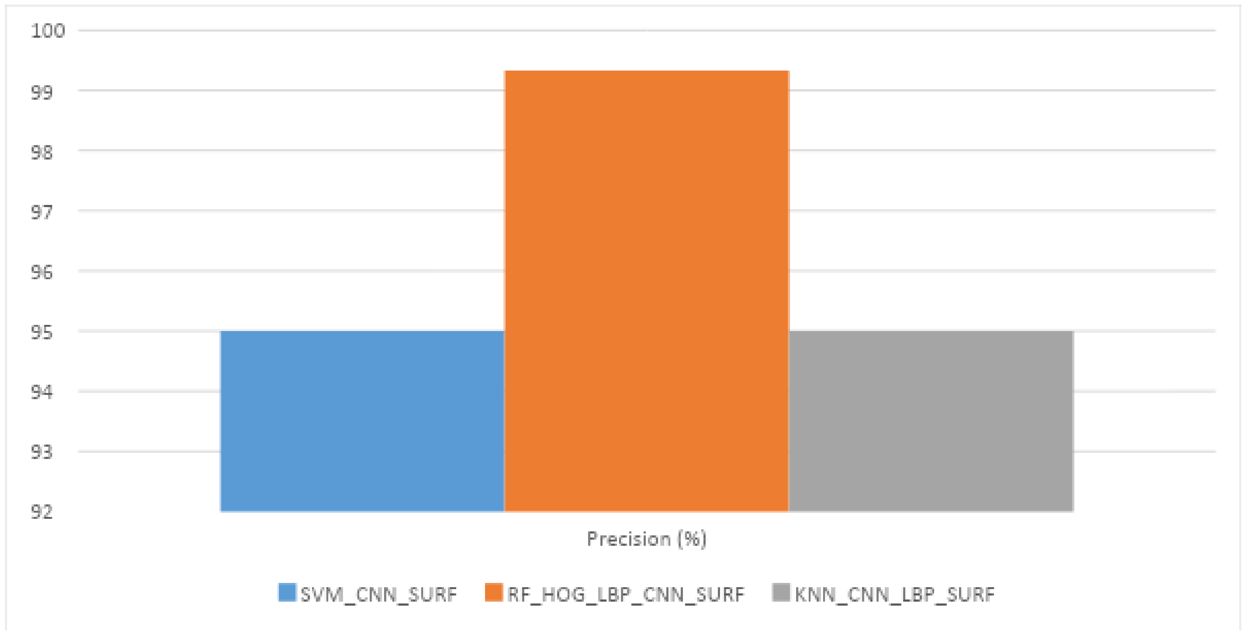
To assess the performance of our system, we used a dataset containing 1500 fundus images of retina that include 900 glaucoma images and 600 healthy images. This dataset was obtained from the Edo Eye Hospital, Pakistan via a Zeiss FF 450 plus fundus camera. The image format was JPG and resolution 2588 × 1958. Among 1500 images, 60% (900 images: 600 Glaucoma and 300 Healthy) dataset was used for the training of all algorithms i.e., SVM, KNN, and RF. However, the remaining 40% (600 images: 300 Glaucoma and 300 Healthy) of data was used for the testing. The results of one best performing combination for each classifier with the various combinations of feature descriptors are reported in

Table 3. The Best Performing Proposed Algorithms on Testing Data.

Method	Precision (%)	Recall (%)	Accuracy (%)	F1 Score (%)
SVM_CNN_SURF	95	95.95	95.5	95.47
RF_HOG_LBP_CNN_SURF	99.33	98.67	99	98.99
KNN_CNN_LBP_SURF	95	93.44	94.16	94.21

SVM performed best with CNN, RF with HOG, CNN, and LBP, and KNN with CNN on testing data. The graph is shown in Figure 5.

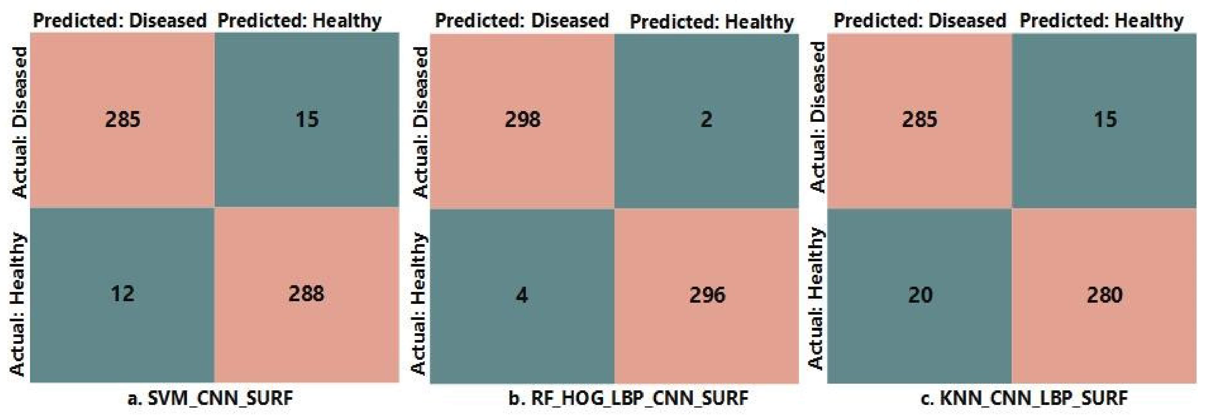
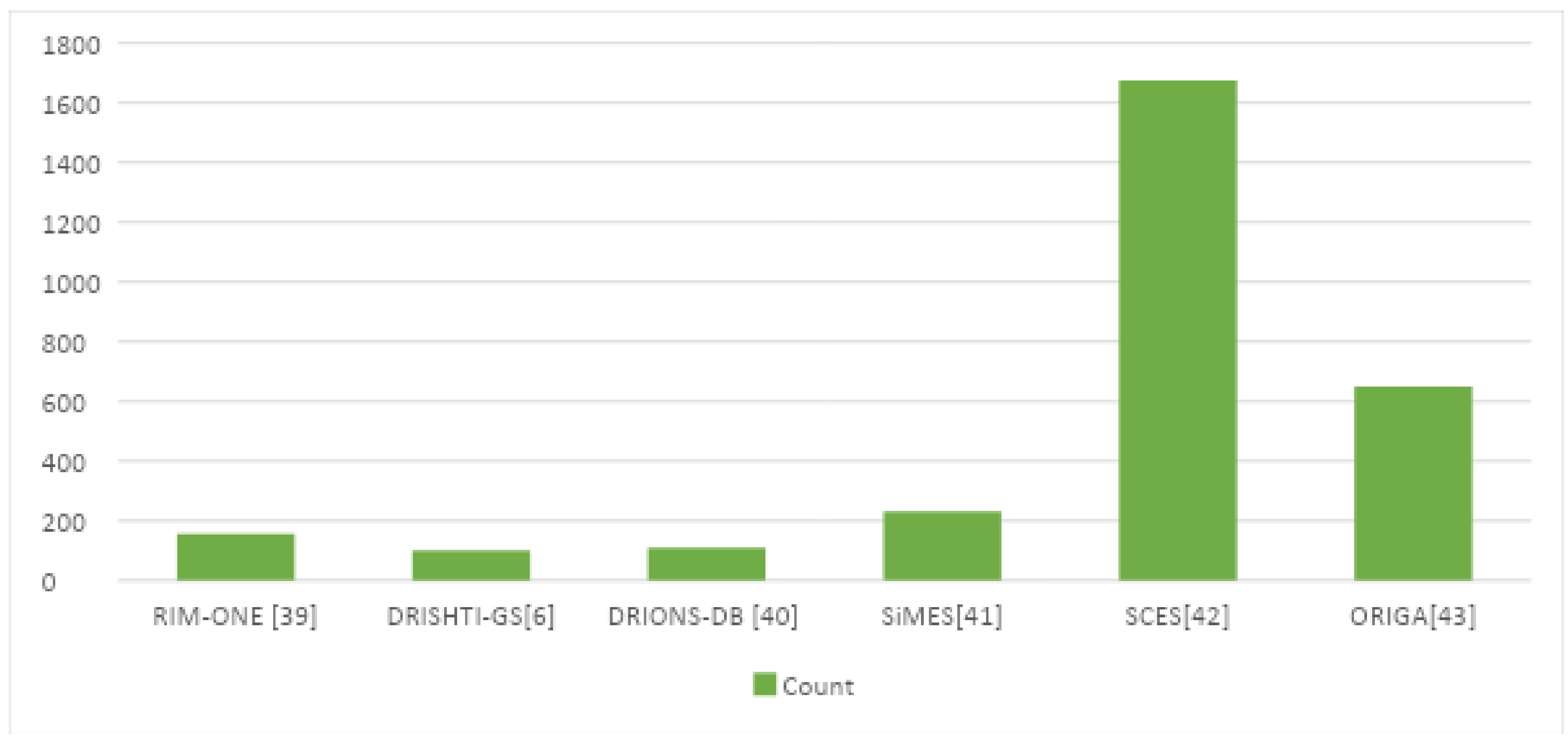
Additionally, confusion matrices are presented in Figure 6 for all three proposed classification methods with specific feature descriptors showing the best performance among all. As in the Figure 6, if the total number of images is 600, then SVM with CNN and SURF classifies 285 as true positive (TP), 288 as true negative (TN), 12 as false positive (FP), and 15 as false negative (FN). More precisely, 285 images are correctly classified as diseased images and 288 images are correctly classified as healthy images by SVM, 12 images are healthy and incorrectly classified as non-healthy, and 15 images are diseased and incorrectly classified as healthy images. Datasets details for glaucoma detection are presented in

Table 4. Datasets Details for the Glaucoma Detection.

Dataset	Count	Type	Purpose	Remarks
RIM-ONE [41]	158	Fundus	Segmentation	Annotated for OC
DRISHTI-GS [6]	101	Fundus	Segmentation	Annotated for OC and OD
DRIONS-DB [42]	110	Fundus	Segmentation	Annotated for OC
SiMES [43]	230	Fundus	Segmentation	OD
SCES [44]	1676 (1630 No Glaucoma, 46 Glaucoma)	Fundus	Classification	Binary Classification
ORIGA [45]	650 (482 No Glaucoma, 168 Glaucoma)	Fundus	Classification	Binary Classification

and the plot is shown in Figure 7.

4.2. Evaluation Metrics

Various metrics have been used for the performance evaluation of the proposed model.

Time: The lowest time is taken by the KNN with an LBP that is 2.3 s as defined in Table 2. The time occupied for the SVM classifier using LBP descriptor is 5.2 s and the minimum time taken for the SVM using CNN descriptor is 2.81 s. The minimum time of RF using the LBP descriptor is 2.4 s as shown in the table.

Accuracy: Accuracy is calculated to examine the performance of the proposed system over the specific data. The technique based on RF with HOG, LBP, CNN, and SURF achieved 98.8% accuracy for the cross-validation and 99% accuracy for the testing data. The equation of accuracy is shown below.

$$Accuracy=\frac{TP+TN}{TP+TN+FP+FN} ,$$

(20)

where true positive (TP) denotes the total images that were classified correctly as non-healthy, whereas false positive (FP) represents the images that were incorrectly classified as positive class such as diseased. The false negative (FN) represents the percentage of images that our proposed method was not able to detect as non-healthy. Moreover, true negative (TN) represents the images that are healthy and classified as healthy by our proposed system. After the RF with CNN, HOG, LBP, and SURF, the SVM algorithm with CNN and SURF feature descriptors performed better, attaining an accuracy of 95.5%.

Recall: Recall R refers to the percentage of the images that were diseased and recalled by the system. The maximum recall was attained by the RF with HOG, CNN, LBP, and SURF feature descriptors, namely 98.67% on testing data. The mathematical equation is shown in Equation (21).

$$R=\frac{TP}{TP+FN}*100 ,$$

(21)

Precision: Precision P refers to the ratio of the frames that are correctly classified through the proposed method. The maximum precision attained by the RF classifier with HOG, CNN, LBP, and SURF is 99.33% on testing data. The equation of precision is presented below:

$$P=\frac{TP}{TP+FP}*100 ,$$

(22)

F1 Score: It is also known as the F Score denoted by F. It represents the accuracy of the model on any dataset. The highest value of the F1 score is 98.9% for RF with a feature descriptor of HOG, CNN, LBP, and SURF. The equation is given below:

$${\mathrm{F}}_1=2. \frac{precision* recall}{precision+recall} ,$$

(23)

4.3. K-Fold Cross Validation

We employed K-fold cross validation [46] as K = {1,2,3,4,5} to evaluate the proposed system’s robustness over the benchmark datasets, i.e., DRISHTI-GS and RIM-ONE [39], for the detection of Glaucoma disease.

DRISHTI-GS consists of 101 retinal fundus images for the segmentation of OC. These images were captured during the medical check-up of the patients in India’s Hospital. The age group of patients was 40–80 years. The images were captured by medical experts who dilated the eyes first and OC at the center. Furthermore, images were taken at the angle of 30 degrees with a view and the format of images was PNG having a resolution of 2996 × 1994.

Moreover, we cross-validated results on the famous dataset RIM-ONE [47] that has been designed by an ophthalmic image group for Glaucoma detection. It is abbreviated as an “Open Retinal Image Database for Optic Nerve Evaluation”. It consists of the fundus images belonging to three Spanish hospitals. We used 100 images for the cross-validation. It was created by four glaucoma experts using the Nidek AFC-210 camera.

Results of cross-validation are reported in

Table 5. Performance of the Proposed Algorithms upon Cross-Validation.

Method	Standard Deviation	Precision (%)	Recall (%)	Accuracy (%)	F1 Score (%)
SVM_LBP	0.0661	88.7	89.8	89.6	89.24
SVM_HOG	0.0653	87.3	90.2	88.7	88.72
SVM_CNN	0.0631	90.6	91.88	91	91.23
SVM_SURF	0.0664	86.7	86.1	87.6
SVM_HOG_CNN	0.0581	88.8	90.3	89.3	89.54
SVM_CNN_SURF	0.066	91.3	91	91.6
SVM_LBP_CNN	0.0600	89.7	91.2	90.2	90.44
SVM_HOG_CNN_LBP	0.0601	89.8	91.3	90.2	90.54
SVM_HOG_CNN_LBP_SURF	0.0521	89.9	90.2	90.7
RF_LBP	0.0655	87.3	89.3	87	88.28
RF_HOG	0.0661	90.1	91.6	90.4	90.84
RF_CNN	0.0651	90.3	92.1	91.2	91.19
RF_SURF	0.0675	89.3	88.1	88.7
RF_HOG_CNN	0.0672	88.7	91.3	89.5	89.98
RF_LBP_CNN	0.0633	89.1	90.8	90	89.94
RF_HOG_CNN_LBP	0.0632	94.1	93.6	93.4
RF_HOG_LBP_CNN_SURF	0.0688	98.4	99.3	98.8	98.9
KNN_LBP	0.0655	85.3	88.3	86.5	86.77
KNN_HOG	0.0661	86.2	89.2	87.3	87.67
KNN_CNN	0.0651	90.3	92.3	91	91.28
KNN_SURF	0.0523	89.3	88.7	89
KNN_HOG_CNN	0.0558	95	98	97	96.47
KNN_LBP_CNN_SURF	0.0512	98.1	98.3	97.8
KNN_LBP_CNN	0.0644	85.8	87.9	86.8	86.83
KNN_HOG_LBP_CNN	0.0610	87.3	90.2	88.7	88.7

. The highest accuracy was attained using RF with HOG, LBP, CNN, and SURF i.e., 98.8%. Simultaneously, the KNN algorithm also performed well with LBP, CNN, and SURF feature descriptors showing an accuracy of 97.8%. The SVM classifier gave the highest accuracy of 91.6% with feature descriptors CNN and SURF. The performance visualization is presented in Figure 8.

4.4. Comparative Analysis with State-of-the-Art

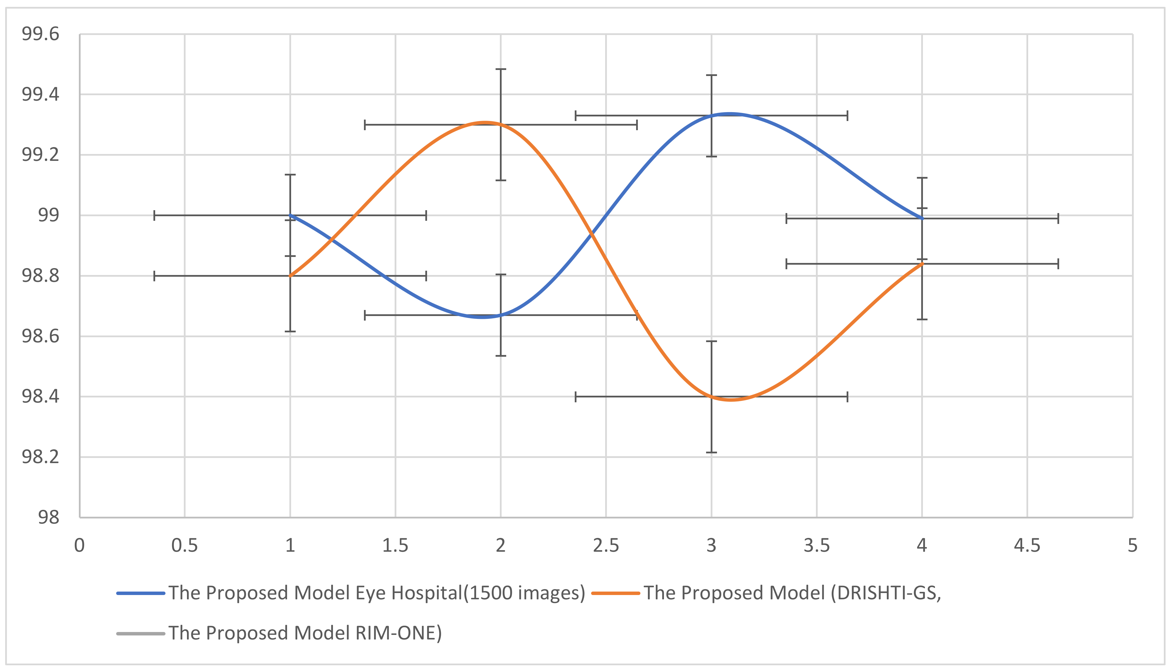
There exist various methods for the detection of glaucoma using existing datasets. Thus, to assess the performance of the proposed system, a comparative analysis is described in

Table 6. Comparative Analysis with State-of-the-Art Techniques.

Reference	Year	Dataset	Accuracy (%)	Recall (%)	Precision (%)	F1Score (%)
[48]	2019	ORIGA	82.80	87.60	77.90
[49]	2017	RIM-ONE V3 DRISHTI-GS	-	-	-	82 85
[50]	2018	SINDI, SCES	84.29(B)	88.78	83.8	-
[51]	2020	RIM-ONE V3 DRISHTI-GS DRIONS-DB	94.8 93.7 93.4	-	-	-
[52]	2019	DRISHTI-GS	-	-	-	82.20(OC)
[53]	2019	DRISHTI-GSI	-	-	-	90.50(OC) 97.10(OD)
The Proposed Model (RF_HOG _CNN_LBP_SURF)	2021	Eye Hospital (1500 images) (DRISHTI-GS, RIM-ONE)	99 98.8	98.67 99.3	99.33 98.4	98.99 98.84

. The comparison reveals that our proposed system outperforms the existing techniques. In [48], ORIGA dataset has been used and 82.80% accuracy has been attained. In [49], two datasets have been used for training and validation, namely RIM-ONE V3 and DRISHTI-GS, attaining the F1 score 82% and 85%, respectively. In [50], SINDI, and SCES datasets have been employed attaining 84.29% accuracy. In [51], datasets such as RIM-ONE V3, DRISHTI-GS, and DRIONS-DB have been employed attaining 94.8%, 93.7%, and 93.4% accuracies respectively. Ref. [52], and [53] utilized the same dataset, i.e., DRISHTI_GSI dataset, achieving an F1 score of 82.20% and 97.10% (maximum based on OD). Our proposed algorithm RF with feature descriptors HOG, CNN, and LBP is based on OD segmentation that consists of OC, giving an accuracy of 99% on testing data and 98.8% on cross-validation. We utilized 1500 images from a well-known hospital for training and testing and DRISHTI-GS, and RIM-ONE for cross-validation. Among all other proposed algorithms, RF_HOG_CNN_LBP_SURF takes a training time of 9 s. Therefore, low-level features have been calculated using HOG, whereas texture-based features have been extracted using the LBP and SURF methods, and high-level features have been extracted using CNN. Additionally, the feature extraction technique selects only the most representative features for the classification. The visualization is presented in Figure 9. The two lines with error bars depict the accuracy, recall, precision, and F1 score concerning datasets.

5. Conclusions

This study aims to detect glaucoma at early stages with the help of a deep learning-based feature descriptor. Fundus images of the retina have been employed for the training and testing of our proposed model. In the first step, images are pre-processed and then the ROI has been extracted using segmentation. Features have been extracted from the region of interest that has the optical disc containing optical cup (OC) through the combination of convolutional neural network (CNN), HOG, LBP, and SURF. Low-level features have been extracted using HOG, texture features have been calculated using LBP and SURF descriptor, whereas high-level features have been extracted using ConvNet. Moreover, we employed a feature selection technique based on ranking, i.e., the MR-MR method, which removes irrelevant features from the extracted features and chooses the most representative features subset. In the end, multi-class classifiers, i.e., SVM, KNN, and RF, have been employed for the classification of the fundus images into healthy and diseased images. Cross-validation was performed on two datasets i.e., DRISHTI-GS and RIM-ONE. The RF classifier with HOG, CNN, LBP, and SURF feature descriptors outperforms the existing algorithms for the detection of glaucoma. Cross-validation has been employed to ensure the robustness of the proposed method. Therefore, the proposed algorithm achieves 98.8% accuracy on cross-validation and 99% accuracy on the testing dataset. The proposed algorithm is robust and can be used for the detection of various diseases. Furthermore, in the future, we aim to employ the proposed method on other disease datasets and try to improve the accuracy. We will reduce the number of feature descriptors and targets to get better results while reducing the complexity of the proposed algorithm. We also aim to rely on the CNN by increasing the number of layers and fine-tuning the parameters to extract the most relevant features from the samples. This will make our model more effective and efficient in terms of performance.

References

- Song, B.J.; Aiello, L.P.; Pasquale, L.R. Presence and risk factors for glaucoma in patients with diabetes. Curr. Diabetes Rep. 2016, 16, 1–13. [Google Scholar] [CrossRef] [PubMed]
- Bhat, S.H.; Kumar, P. Segmentation of Optic Disc by Localized Active Contour Model in Retinal Fundus Image. In Smart Innovations in Communication and Computational Sciences; Springer: Berlin/Heidelberg, Germany, 2019; pp. 35–44. [Google Scholar]
- Khan, M.A.; Ashraf, I.; Alhaisoni, M.; Damaševičius, R.; Scherer, R.; Rehman, A.; Bukhari, S.A. Multimodal brain tumor classification using deep learning and robust feature selection: A machine learning application for radiologists. Diagnostics 2020, 10, 565. [Google Scholar] [CrossRef]
- Singh, L.K.; Garg, H. Detection of Glaucoma in Retinal Fundus Images Using Fast Fuzzy C means clustering approach. In Proceedings of the 2019 International Conference on Computing, Communication, and Intelligent Systems (ICCCIS), Greater Noida, India, 18–19 October 2019; pp. 397–403. [Google Scholar] [CrossRef]
- Kosior-Jarecka, E.; Pankowska, A.; Polit, P.; Stępniewski, A.; Symms, M.R.; Kozioł, P.; Pietura, R. Volume of lateral geniculate nucleus in patients with Glaucoma in 7Tesla MRI. J. Clin. Med. 2020, 9, 2382. [Google Scholar] [CrossRef]
- Sivaswamy, J.; Krishnadas, S.R.; Joshi, G.D.; Jain, M.; Tabish, A.U.S. Drishti-GS: Retinal image dataset for optic nerve head(ONH) segmentation. In Proceedings of the 2014 IEEE 11th International Symposium on Biomedical Imaging (ISBI), Beijing, China, 29 April–2 May 2014; pp. 53–56. [Google Scholar] [CrossRef] [Green Version]
- Sivaswamy, J.; Krishnadas, S.; Chakravarty, A.; Joshi, G.; Tabish, A.S. A comprehensive retinal image dataset for the assessment of glaucoma from the optic nerve head analysis. JSM Biomed. Imaging Data Pap. 2015, 2, 1004. [Google Scholar]
- Walter, T.; Klein, J.-C.; Massin, P.; Erginay, A. A contribution of image processing to the diagnosis of diabetic retinopa-thy-detection of exudates in color fundus images of the human retina. IEEE Trans. Med. Imaging 2002, 21, 1236–1243. [Google Scholar] [CrossRef] [PubMed]
- Tang, Y.; Ren, F.; Pedrycz, W. Fuzzy C-Means clustering through SSIM and patch for image segmentation. Appl. Soft Comput. 2019, 87, 105928. [Google Scholar] [CrossRef]
- Zhu, Q.; Wang, Y.; Du, B.; Yan, P. OASIS: One-pass aligned atlas set for medical image segmentation. Neurocomputing 2021, 470, 130–138. [Google Scholar] [CrossRef]
- Chrastek, R.; Niemann, H.; Kubecka, L.; Jan, J.; Derhartunian, V.; Michelson, G. Optic Nerve Head Segmentation in Multi-Modal Retinal Images. In Medical Imaging 2005: Image Processing, 2005, Vol. 5747; International Society for Optics and Photonics: Bellingham, WA, USA; pp. 1604–1615.
- Lu, S. Accurate and Efficient Optic Disc Detection and Segmentation by a Circular Transformation. IEEE Trans. Med. Imaging 2011, 30, 2126–2133. [Google Scholar] [CrossRef]
- Soorya, M.; Issac, A.; Dutta, M.K. Automated Framework for Screening of Glaucoma Through Cloud Computing. J. Med. Syst. 2019, 43, 136. [Google Scholar] [CrossRef]
- Singh, L.K.; Khanna, M.; Garg, H. Multimodal Biometric Based on Fusion of Ridge Features with Minutiae Features and Face Features. Int. J. Inf. Syst. Model. Des. 2020, 11, 37–57. [Google Scholar] [CrossRef]
- Singh, L.K.; Garg, H.; Khanna, M.; Bhadoria, R.S. An enhanced deep image model for glaucoma diagnosis using fea-ture-based detection in retinal fundus. Med. Biol. Eng. Comput. 2021, 59, 333–353. [Google Scholar] [CrossRef] [PubMed]
- Wong, D.W.; Liu, J.; Lim, J.H.; Jia, X.; Yin, F.; Li, H.; Wong, T.Y. Level-set based automatic cup-to-disc ratio determination using retinal fundus images in ARGALI. In Proceedings of the 2008 30th Annual International Conference of the IEEE Engineering in Medicine and Biology Society, Vancouver, BC, Canada, 20–25 August 2008; pp. 2266–2269. [Google Scholar]
- Joshi, G.D.; Sivaswamy, J.; Karan, K.; Krishnadas, S. Optic disk and cup boundary detection using regional information. In Proceedings of the 2010 IEEE International Symposium on Biomedical Imaging: From Nano to Macro, Rotterdam, The Netherlands, 14–17 April 2010; pp. 948–951. [Google Scholar]
- Cheng, J.; Liu, J.; Xu, Y.; Yin, F.; Wong, D.W.K.; Tan, N.-M.; Tao, D.; Cheng, C.-Y.; Aung, T.; Wong, T.Y. Superpixel Classification Based Optic Disc and Optic Cup Segmentation for Glaucoma Screening. IEEE Trans. Med. Imaging 2013, 32, 1019–1032. [Google Scholar] [CrossRef]
- Raghavendra, U.; Fujita, H.; Bhandary, S.V.; Gudigar, A.; Tan, J.H.; Acharya, U.R. Deep convolution neural network for accurate diagnosis of glaucoma using digital fundus images. Inf. Sci. 2018, 441, 41–49. [Google Scholar] [CrossRef]
- Li, A.; Cheng, J.; Wong, D.W.K.; Liu, J. Integrating holistic and local deep features for glaucoma classification. In Proceedings of the 2016 38th Annual International Conference of the IEEE Engineering in Medicine and Biology Society (EMBC), Orlando, FL, USA, 16–20 August 2016; pp. 1328–1331. [Google Scholar]
- Chen, X.; Xu, Y.; Wong, D.W.K.; Wong, T.Y.; Liu, J. Glaucoma detection based on deep convolutional neural network. In Proceedings of the 2015 37th Annual International Conference of the IEEE Engineering in Medicine and Biology Society (EMBC), Milan, Italy, 25–29 August 2015; pp. 715–718. [Google Scholar]
- Chen, X.; Xu, Y.; Yan, S.; Wong, D.W.K.; Wong, T.Y.; Liu, J. Automatic feature learning for glaucoma detection based on deep learning. In Proceedings of the International Conference on Medical Image Computing and Computer-Assisted Intervention, Munich, Germany, 5–9 October 2015; pp. 669–677. [Google Scholar]
- Orlando, J.I.; Prokofyeva, E.; del Fresno, M.; Blaschko, M.B. Convolutional neural network transfer for automated glau-coma identification. In Proceedings of the 12th International Symposium on Medical Information Processing and Analysis, Tandil, Argentina, 5–7 December 2016; Volume 10160. [Google Scholar]
- Chai, Y.; He, L.; Mei, Q.; Liu, H.; Xu, L. Deep Learning Through Two-Branch Convolutional Neuron Network for Glaucoma Diagnosis. In Proceedings of the International Conference on Smart Health, Hong Kong, China, 26–27 June 2017; pp. 191–201. [Google Scholar] [CrossRef]
- Shankaranarayana, S.M.; Ram, K.; Mitra, K.; Sivaprakasam, M. Joint optic disc and cup segmentation using fully convolutional and adversarial networks. In Fetal, Infant and Ophthalmic Medical Image Analysis; Springer: Berlin/Heidelberg, Germany, 2017; pp. 168–176. [Google Scholar]
- Zilly, J.; Buhmann, J.M.; Mahapatra, D. Glaucoma detection using entropy sampling and ensemble learning for automatic optic cup and disc segmentation. Comput. Med. Imaging Graph. 2017, 55, 28–41. [Google Scholar] [CrossRef]
- Panda, R.; Puhan, N.B.; Rao, A.; Mandal, B.; Padhy, D.; Panda, G. Deep convolutional neural network-based patch classification for retinal nerve fiber layer defect detection in early glaucoma. J. Med. Imaging 2018, 5, 044003. [Google Scholar] [CrossRef] [PubMed]
- Shibata, N.; Tanito, M.; Mitsuhashi, K.; Fujino, Y.; Matsuura, M.; Murata, H.; Asaoka, R. Development of a deep residual learning algorithm to screen for glaucoma from fundus photography. Sci. Rep. 2018, 8, 1–9. [Google Scholar] [CrossRef] [PubMed] [Green Version]
- Raghavendra, U.; Gudigar, A.; Bhandary, S.V.; Rao, T.N.; Ciaccio, E.J.; Acharya, U.R. A Two Layer Sparse Autoencoder for Glaucoma Identification with Fundus Images. J. Med. Syst. 2019, 43, 1–9. [Google Scholar] [CrossRef]
- Kim, S.J.; Cho, K.J.; Oh, S. Development of machine learning models for diagnosis of glaucoma. PLoS ONE 2017, 12, e0177726. [Google Scholar] [CrossRef] [Green Version]
- Asaoka, R.; Murata, H.; Iwase, A.; Araie, M. Detecting preperimetric glaucoma with standard automated perimetry using a deep learning classifier. Ophthalmology 2016, 123, 1974–1980. [Google Scholar] [CrossRef]
- Li, Z.; He, Y.; Keel, S.; Meng, W.; Chang, R.T.; He, M. Efficacy of a Deep Learning System for Detecting Glaucomatous Optic Neuropathy Based on Color Fundus Photographs. Ophthalmology 2018, 125, 1199–1206. [Google Scholar] [CrossRef] [Green Version]
- Maninis, K.-K.; Pont-Tuset, J.; Arbeláez, P.; van Gool, L. Deep retinal image understanding. In Proceedings of the International Conference on Medical Image Computing and Computer-Assisted Intervention, Athens, Greece, 17–21 October 2016; pp. 140–148. [Google Scholar]
- Tan, J.H.; Acharya, U.R.; Bhandary, S.; Chua, K.C.; Sivaprasad, S. Segmentation of optic disc, fovea and retinal vasculature using a single convolutional neural network. J. Comput. Sci. 2017, 20, 70–79. [Google Scholar] [CrossRef] [Green Version]
- Srivastava, R.; Cheng, J.; Wong, D.W.K.; Liu, J. Using deep learning for robustness to parapapillary atrophy in optic disc segmentation. In Proceedings of the 2015 IEEE 12th International Symposium on Biomedical Imaging (ISBI), Brooklyn, NY, USA, 16–19 April 2015; pp. 768–771. [Google Scholar] [CrossRef]
- Novotny, A.; Odstrcilik, J.; Kolar, R.; Jan, J. Texture analysis of nerve fibre layer in retinal images via local binary patterns and Gaussian Markov random fields. In Proceedings of the 20th Biennial International EURASIP Conference (BIOSIGNAL’10), Brno, Czech Republic, 27–29 June 2010; pp. 308–315. [Google Scholar]
- Zhang, Z.; Liu, J.; Wong, W.K.; Tan, N.M.; Lim, J.H.; Lu, S.; Li, H.; Liang, Z.; Wong, T.Y. Neuro-retinal optic cup detection in glaucoma diagnosis. In Proceedings of the 2009 2nd International Conference on Biomedical Engineering and Informatics, Tianjin, China, 17–19 October 2009; pp. 1–4. [Google Scholar]
- Qureshi, I. Glaucoma detection in retinal images using image processing techniques: A survey. Int. J. Adv. Netw. Appl. 2015, 7, 2705. [Google Scholar]
- Acharya, U.R.; Dua, S.; Du, X.; Chua, C.K. Automated Diagnosis of Glaucoma Using Texture and Higher Order Spectra Features. IEEE Trans. Inf. Technol. Biomed. 2011, 15, 449–455. [Google Scholar] [CrossRef]
- Bay, H.; Tuytelaars, T.; van Gool, L. Surf: Speeded up robust features. In Proceedings of the European Conference on Computer Vision, Graz, Austria, 7–13 May 2006; pp. 404–417. [Google Scholar]
- Peng, H.; Long, F.; Ding, C. Pattern Anal Mach Intell. IEEE Trans. 2005, 27, 1226. [Google Scholar]
- Carmona, E.J.; Rincón, M.; García-Feijoó, J.; Martínez-de-la-Casa, J.M. Identification of the optic nerve head with genet-ic algorithms. Artif. Intell. Med. 2008, 43, 243–259. [Google Scholar] [CrossRef] [PubMed]
- Foong, A.W.P.; Saw, S.-M.; Loo, J.-L.; Shen, S.; Loon, S.-C.; Rosman, M.; Aung, T.; Tan, D.T.H.; Tai, E.S.; Wong, T.Y. Rationale and Methodology for a Population-Based Study of Eye Diseases in Malay People: The Singapore Malay Eye Study (SiMES). Ophthalmic Epidemiol. 2007, 14, 25–35. [Google Scholar] [CrossRef] [PubMed]
- Sng, C.; Foo, L.-L.; Cheng, C.-Y.; Allen, J.C.; He, M.; Krishnaswamy, G.; Nongpiur, M.E.; Friedman, D.S.; Wong, T.Y.; Aung, T. Determinants of Anterior Chamber Depth: The Singapore Chinese Eye Study. Ophthalmology 2012, 119, 1143–1150. [Google Scholar] [CrossRef]
- Zhang, Z.; Yin, F.S.; Liu, J.; Wong, W.K.; Tan, N.M.; Lee, B.H.; Cheng, J.; Wong, T.Y. Origa-light: An online retinal fundus image database for glaucoma analysis and research. In Proceedings of the 2010 Annual International Conference of the IEEE Engineering in Medicine and Biology, Buenos Aires, Argentina, 31 August–4 September 2010; pp. 3065–3068. [Google Scholar]
- Yadav, S.; Shukla, S. Analysis of k-fold cross-validation over hold-out validation on colossal datasets for quality classification. In Proceedings of the 2016 IEEE 6th International Conference on Advanced Computing (IACC), Bhimavaram, India, 27–28 February 2016; pp. 78–83. [Google Scholar]
- Fumero, F.; Alayón, S.; Sanchez, J.L.; Sigut, J.; Gonzalez-Hernandez, M. RIM-ONE: An open retinal image database for optic nerve evaluation. In Proceedings of the 2011 24th International Symposium on Computer-Based Medical Systems (CBMS), Bristol, UK, 27–30 June 2011; pp. 1–6. [Google Scholar]
- Zhao, X.; Guo, F.; Mai, Y.; Tang, J.; Duan, X.; Zou, B.; Jiang, L. Glaucoma screening pipeline based on clinical measurements and hidden features. IET Image Process. 2019, 13, 2213–2223. [Google Scholar] [CrossRef]
- Sevastopolsky, A. Optic disc and cup segmentation methods for glaucoma detection with modification of U-Net convolutional neural network. Pattern Recognit. Image Anal. 2017, 27, 618–624. [Google Scholar] [CrossRef] [Green Version]
- Fu, H.; Cheng, J.; Xu, Y.; Wong, D.W.K.; Liu, J.; Cao, X. Joint Optic Disc and Cup Segmentation Based on Multi-Label Deep Network and Polar Transformation. IEEE Trans. Med. Imaging 2018, 37, 1597–1605. [Google Scholar] [CrossRef] [Green Version]
- Bhatkalkar, B.; Joshi, A.; Prabhu, S.; Bhandary, S. Automated fundus image quality assessment and segmentation of optic disc using convolutional neural networks. Int. J. Electr. Comput. Eng. (IJECE) 2020, 10, 816–827. [Google Scholar] [CrossRef] [Green Version]
- Gao, Y.; Yu, X.; Wu, C.; Zhou, W.; Wang, X.; Chu, H. Accurate and Efficient Segmentation of Optic Disc and Optic Cup in Retinal Images Integrating Multi-View Information. IEEE Access 2019, 7, 148183–148197. [Google Scholar] [CrossRef]
- Jiang, Y.; Duan, L.; Cheng, J.; Gu, Z.; Xia, H.; Fu, H.; Li, C.; Liu, J. JointRCNN: A Region-Based Convolutional Neural Network for Optic Disc and Cup Segmentation. IEEE Trans. Biomed. Eng. 2019, 67, 335–343. [Google Scholar] [CrossRef] [PubMed]