
Deep Feature Vectors Concatenation for Eye Disease Detection Using Fundus Image

 ,
,
Abstract
:1. Introduction
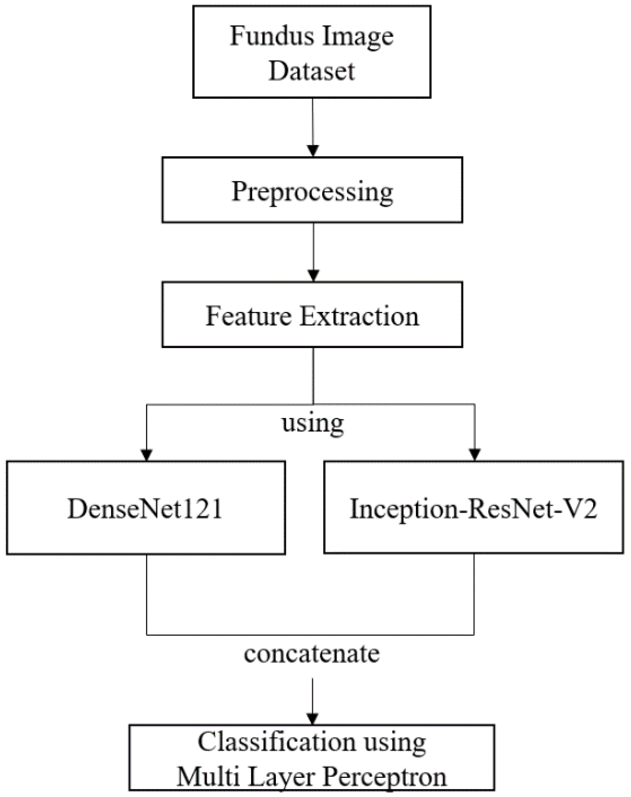
2. Materials and Methods
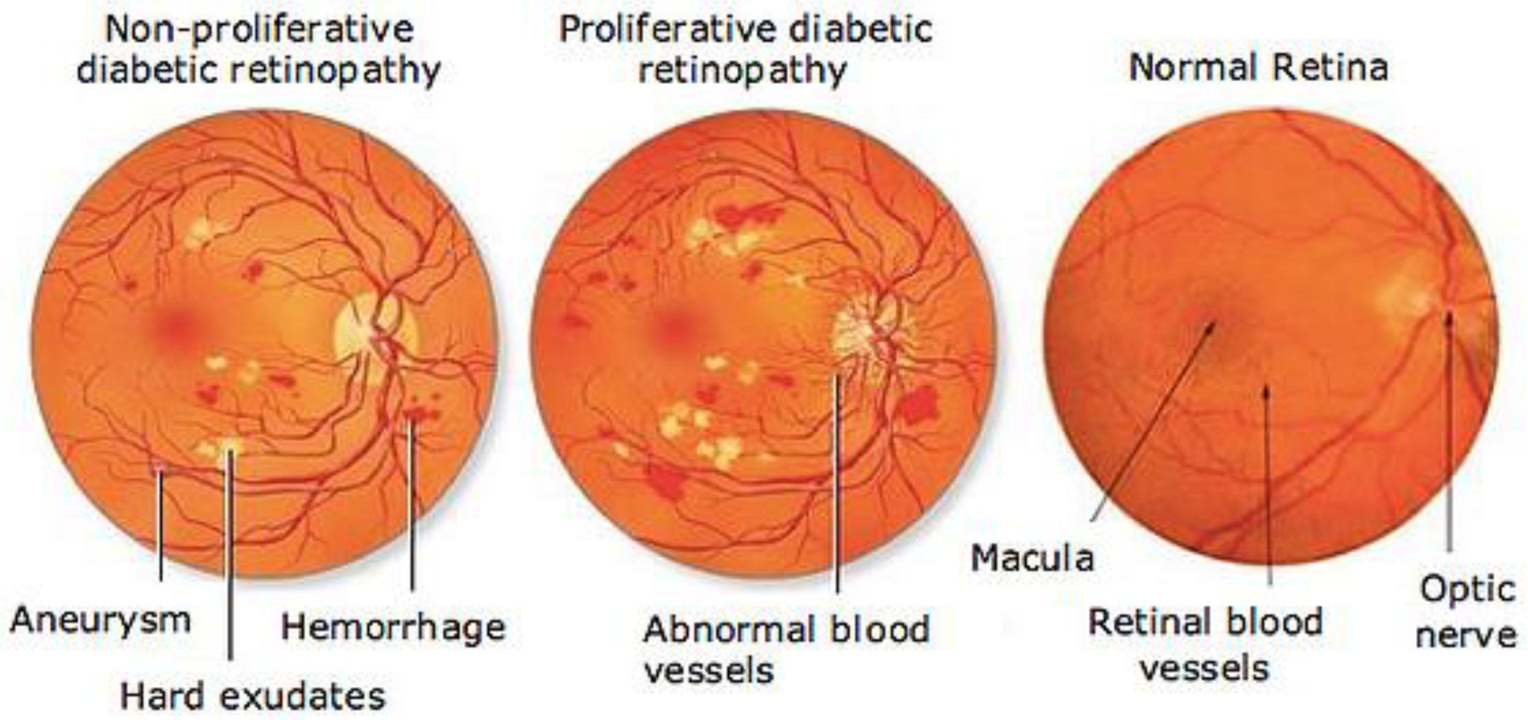
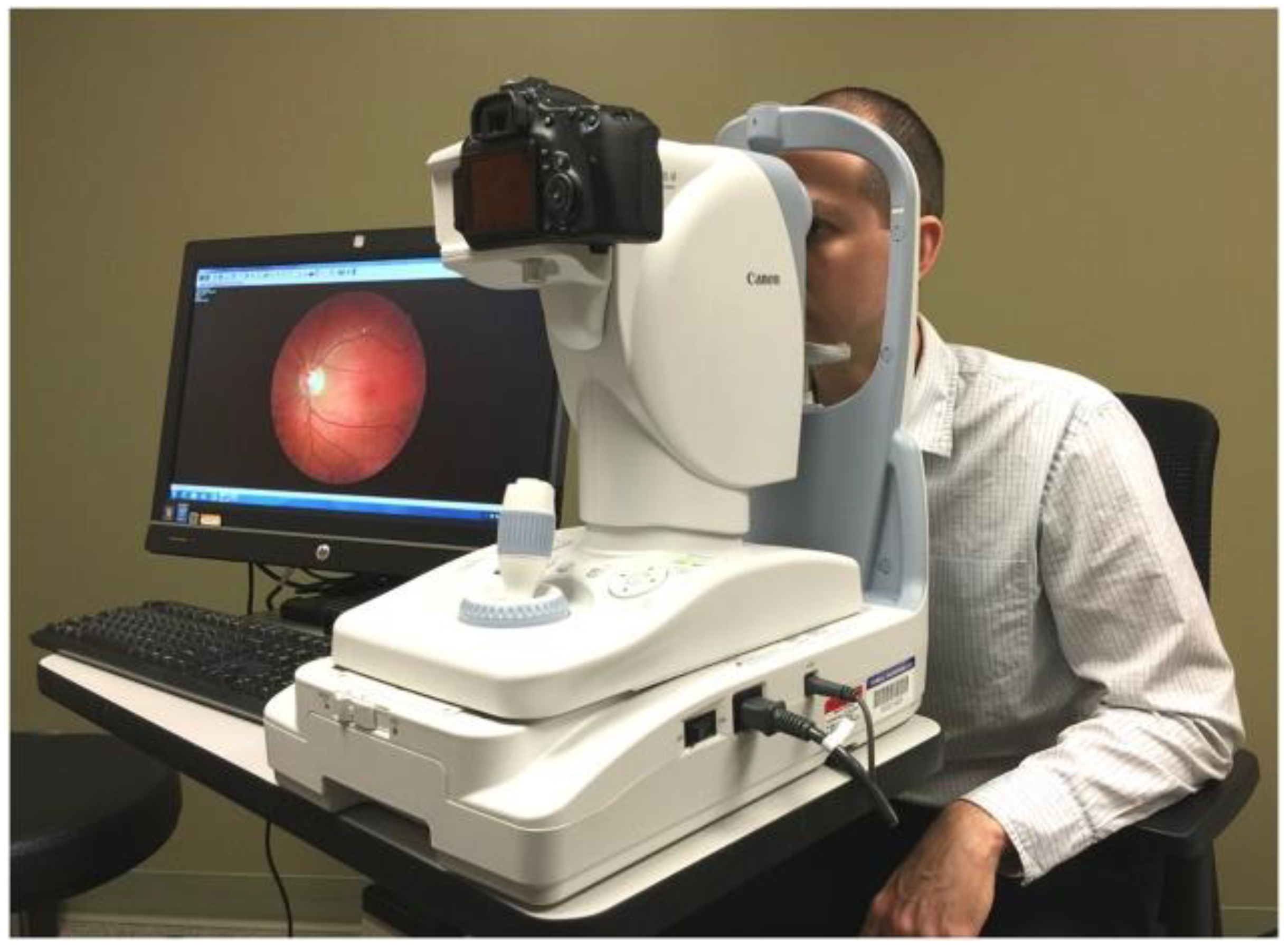
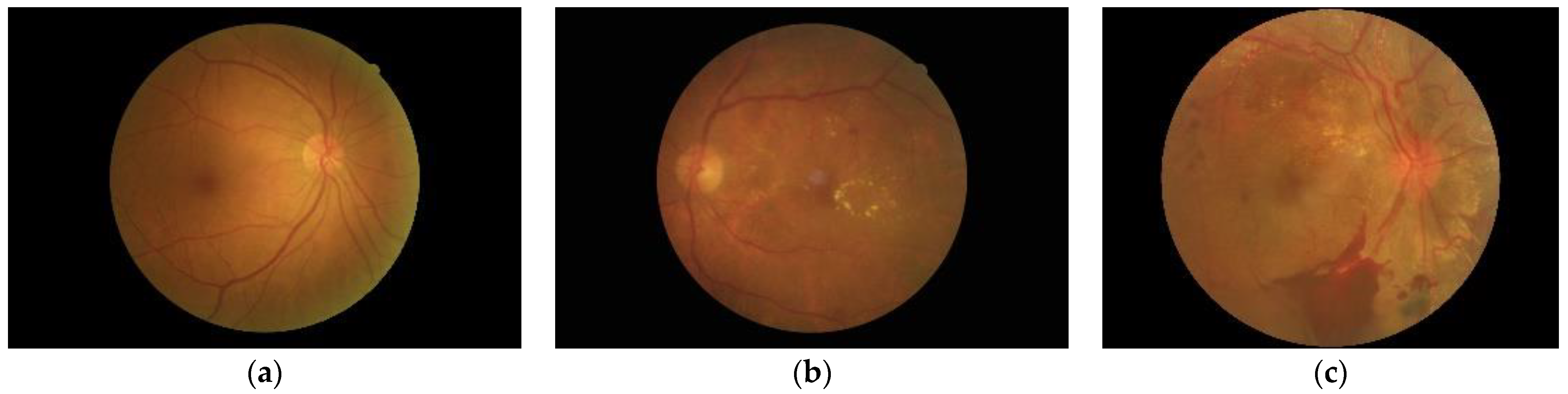
2.1. Fundus Image Dataset
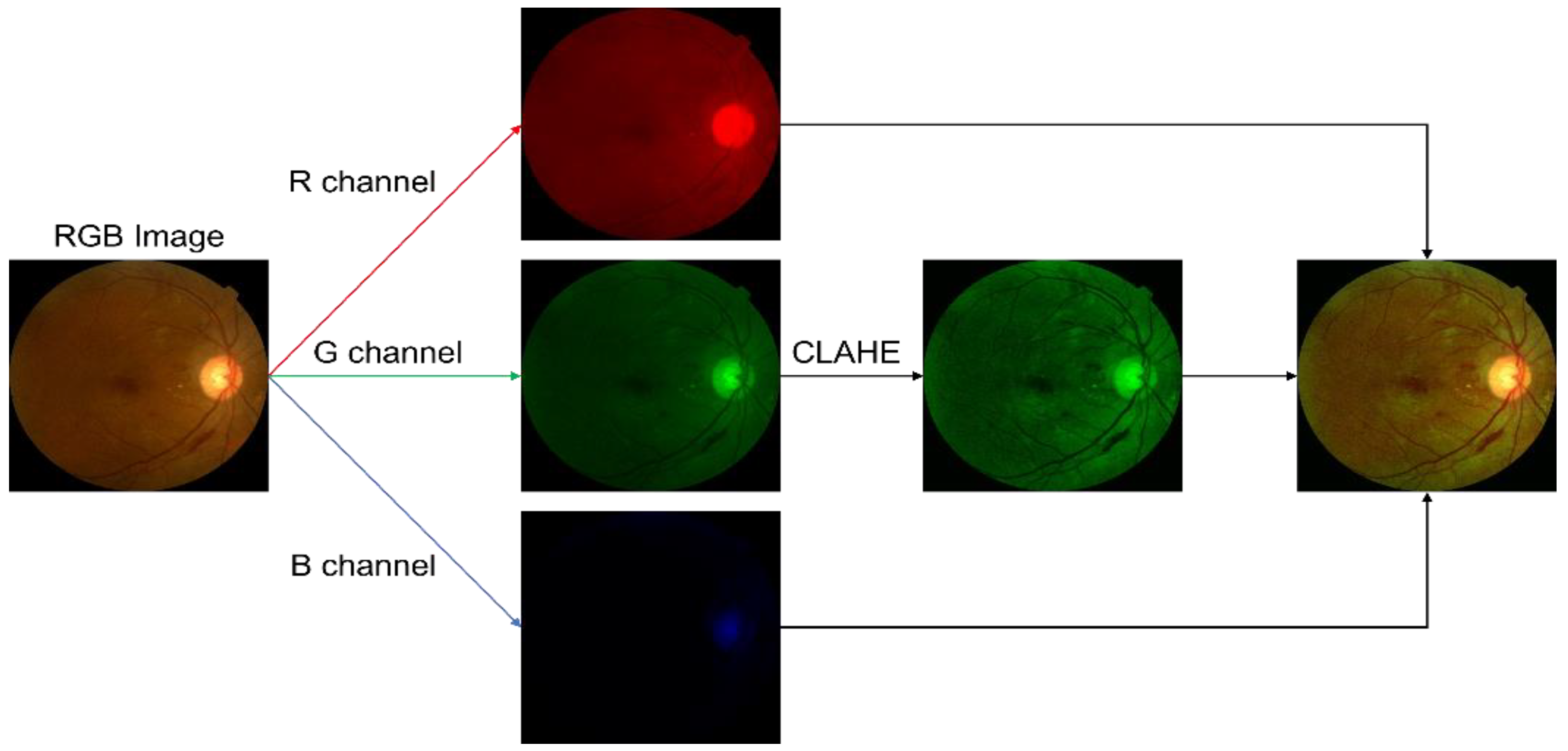
2.2. Preprocessing
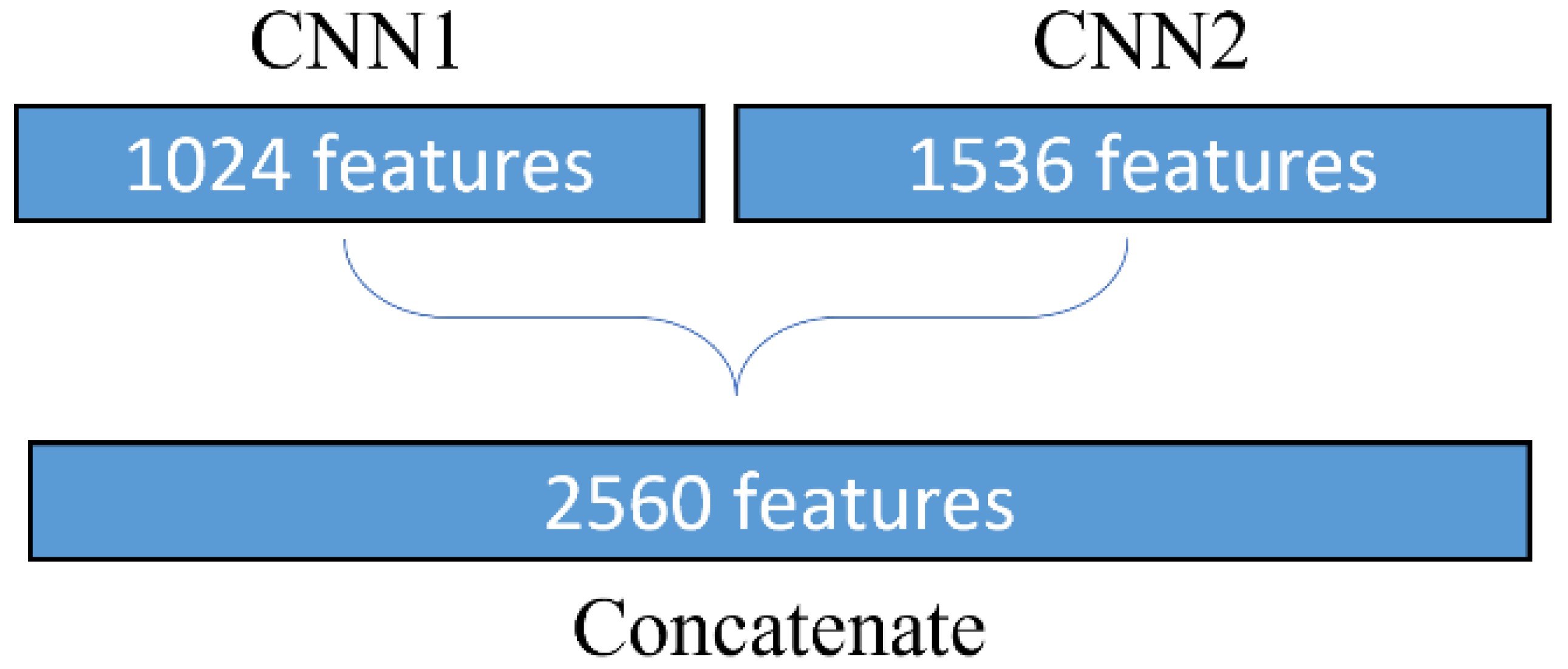
2.3. Deep Feature Vector
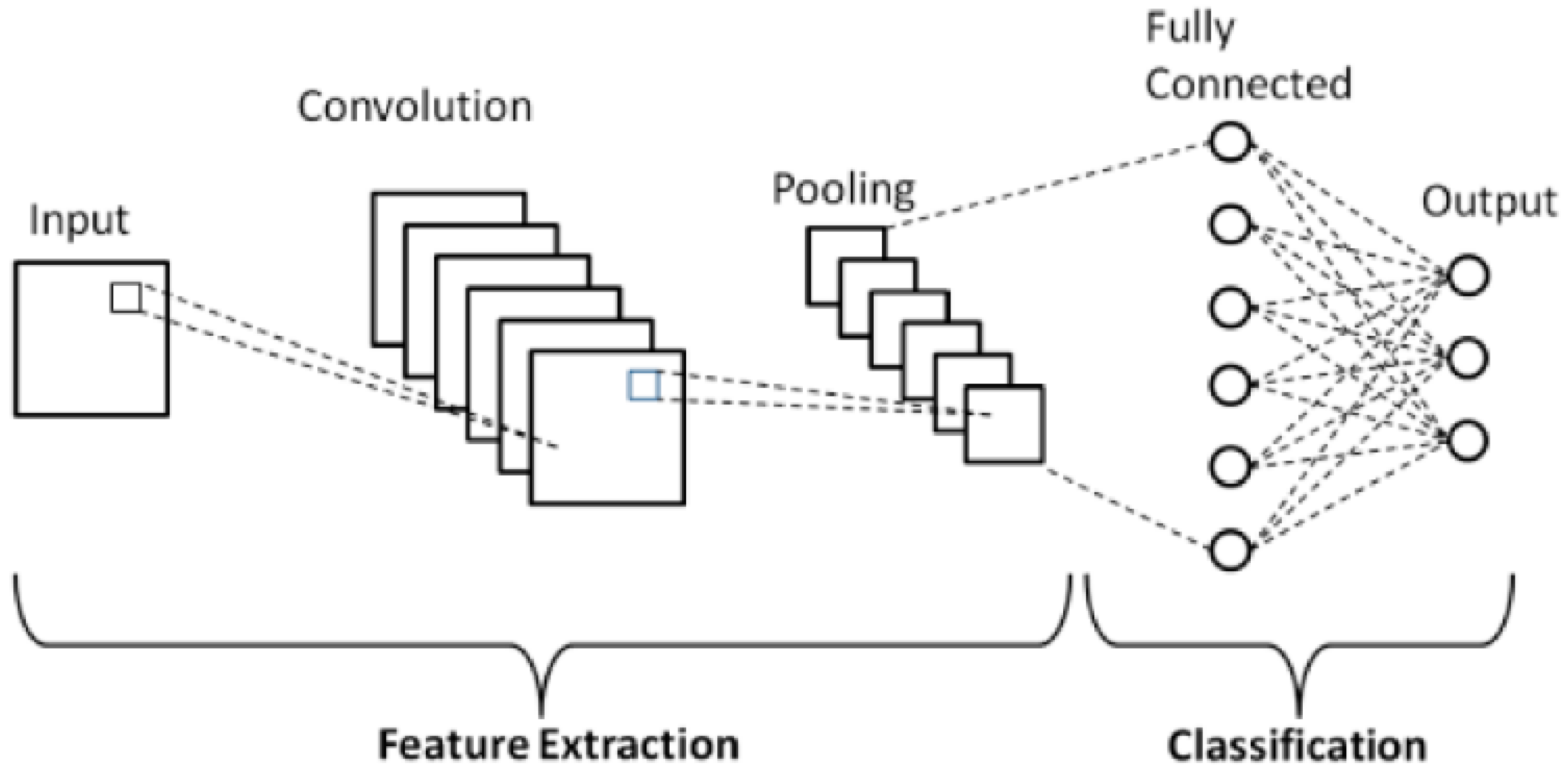
2.3.1. Convolutional Neural Network
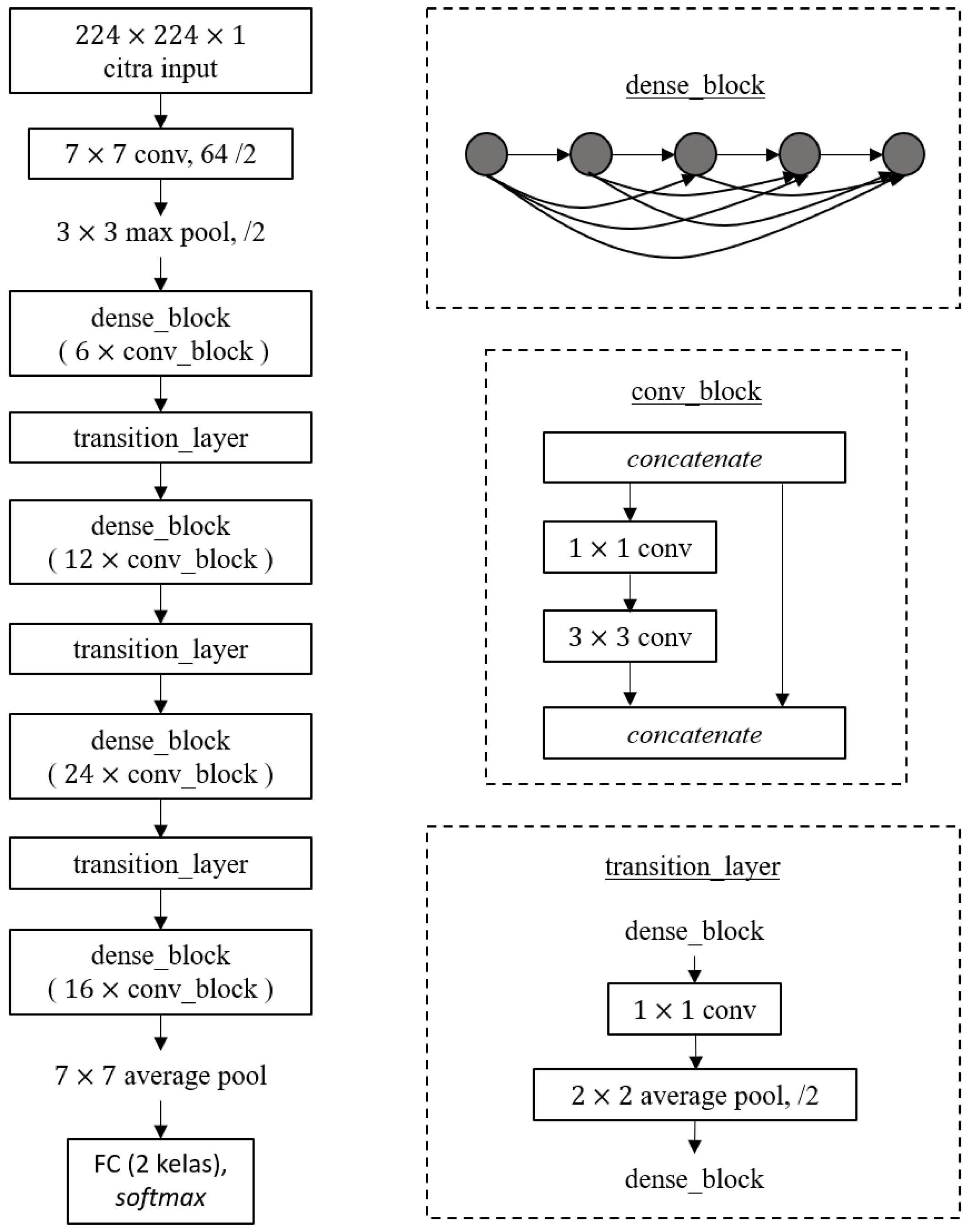
2.3.2. DenseNet121
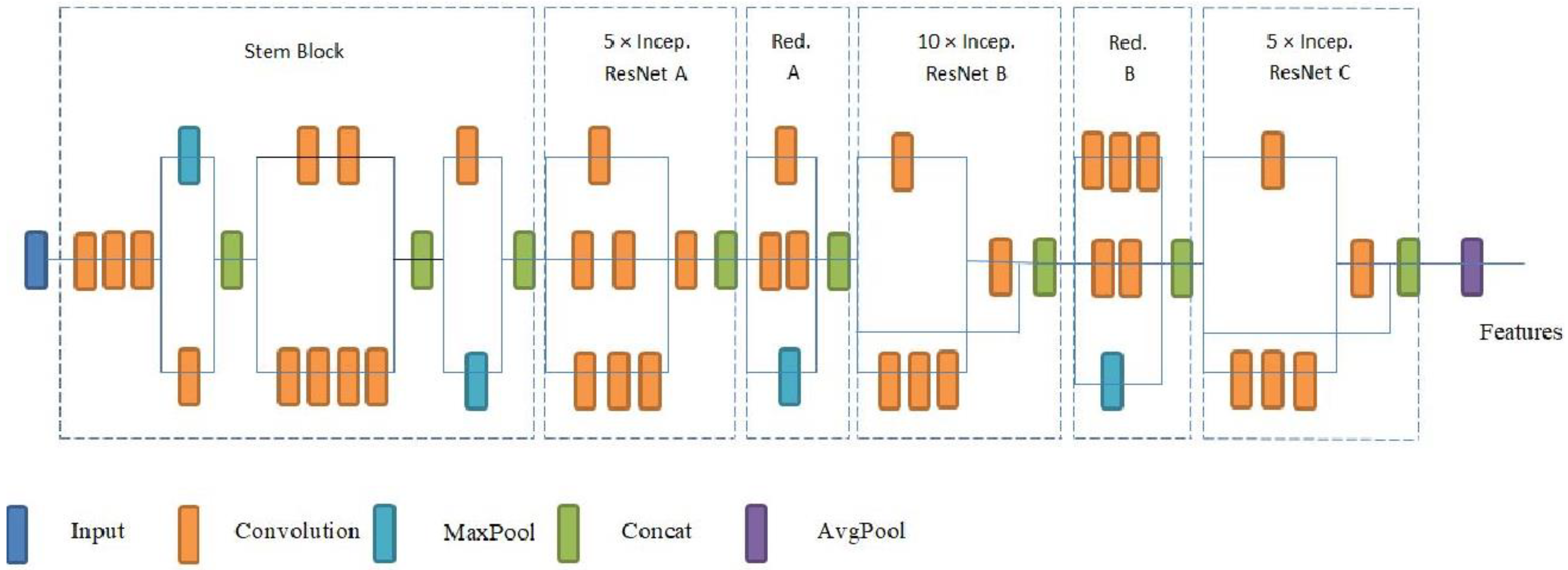
2.3.3. Inception-ResNetV2


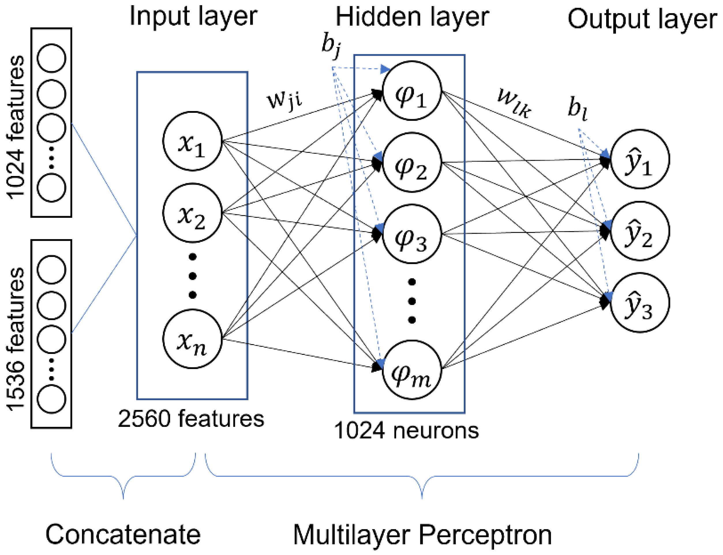
2.4. Classification
Multilayer Perceptron (MLP)
2.5. Experimental Setup
2.5.1. System Specifications
- RAM: 13 GB
- Memory: 32 GB
- GPU: Nvidia Tesla K80 with 16 GB memory, CUDA version 11.2
- -
- Number of sockets: one (available slots for physical processors)
- -
- Number of cores each processor has: one core(s) per socket
- -
- Number of threads each core has: two thread(s) per core
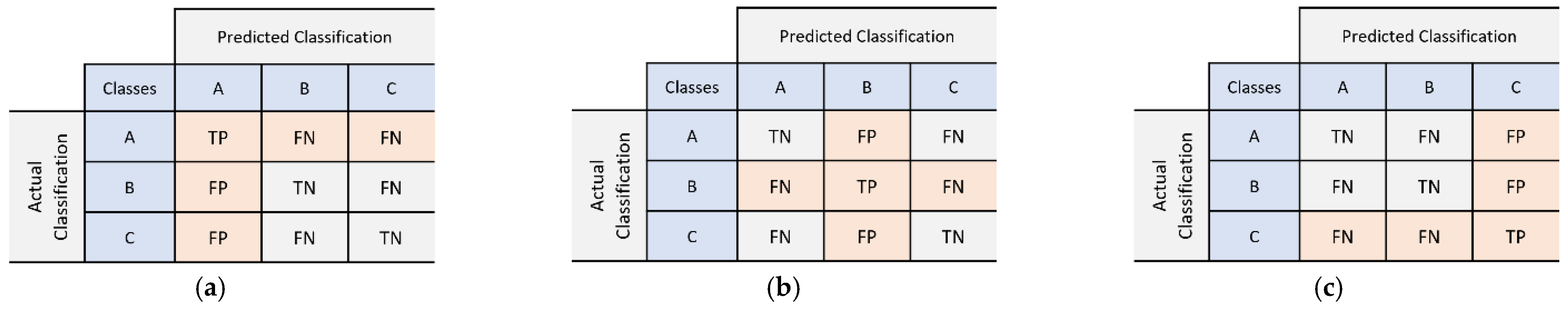
2.5.2. Evaluation Metrics
2.5.3. Hyperparameter Tuning
3. Results
3.1. Preprocessing Implementation
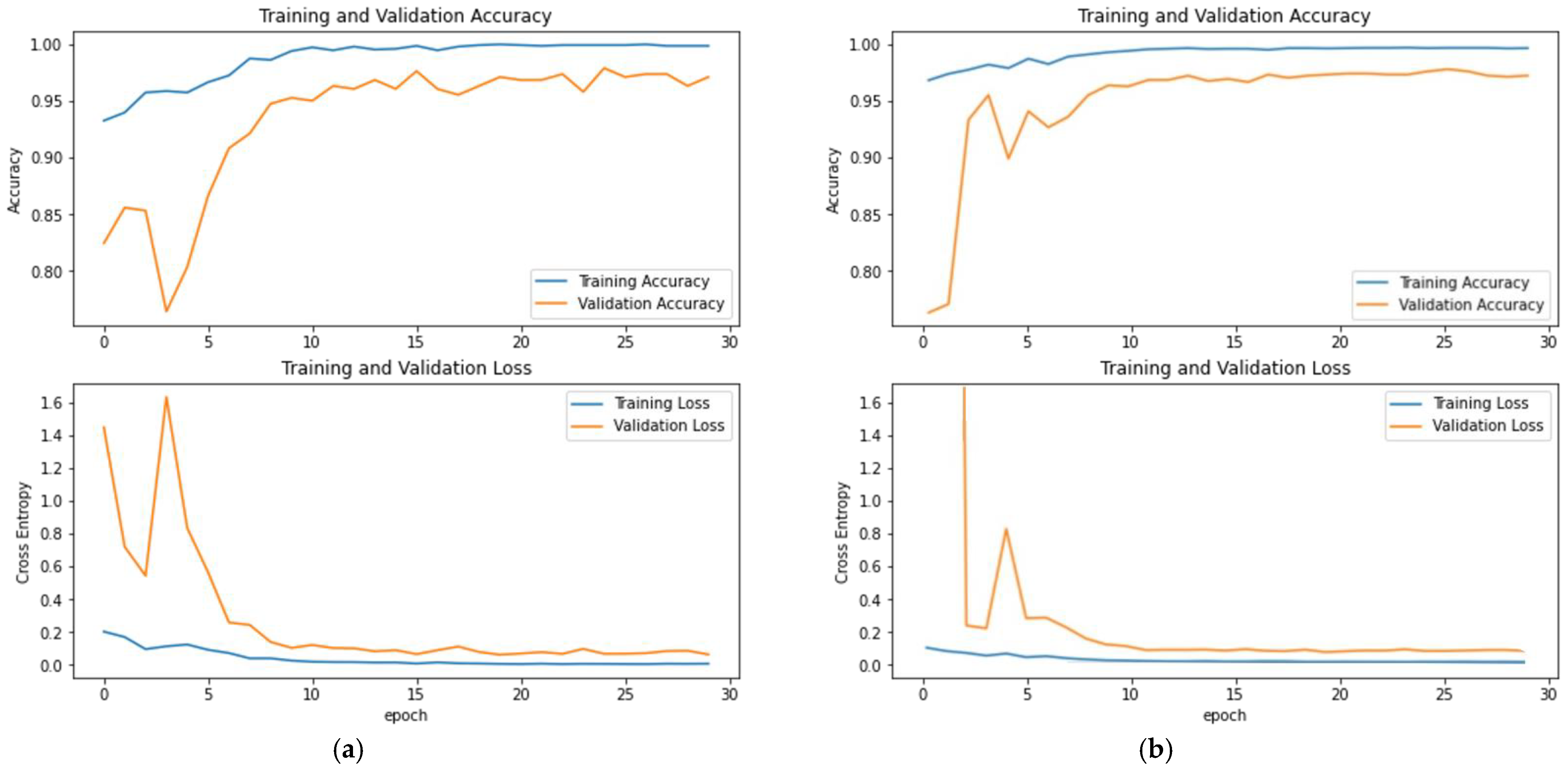
3.2. Evaluation of DenseNet121 and Inception-ResNetV2
4. Discussion
5. Conclusions
Author Contributions
Funding
Institutional Review Board Statement
Informed Consent Statement
Data Availability Statement
Acknowledgments
Conflicts of Interest
References
- Sperling, M.A.; Tamborlane, W.V.; Battelino, T.; Weinzimer, S.A.; Phillip, M. CHAPTER 19—Diabetes mellitus. In Pediatric Endocrinology, 4th ed.; Sperling, M.A., Ed.; W.B. Saunders: Philadelphia, PA, USA, 2014; pp. 846–900.e841. [Google Scholar]
- Saeedi, P.; Petersohn, I.; Salpea, P.; Malanda, B.; Karuranga, S.; Unwin, N.; Colagiuri, S.; Guariguata, L.; Motala, A.A.; Ogurtsova, K.; et al. Global and regional diabetes prevalence estimates for 2019 and projections for 2030 and 2045: Results from the International Diabetes Federation Diabetes Atlas, 9th edition. Diabetes Res. Clin. Pract. 2019, 157, 107843. [Google Scholar] [CrossRef] [PubMed] [Green Version]
- Ohiagu, F.O.; Chikezie, P.C.; Chikezie, C.M. Pathophysiology of diabetes mellitus complications: Metabolic events and control. Biomed. Res. Ther. 2021, 8, 4243–4257. [Google Scholar] [CrossRef]
- Adelson, J.; Rupert, R.A.B.; Briant, P.S.; Flaxman, S.; Taylor, H.; Jonas, J.B. Causes of Blindness and Vision Impairment in 2020 and Trends over 30 Years: Evaluating the Prevalence of Avoidable Blindness in Relation to “VISION 2020: The Right to Sight”. Available online: https://www.iapb.org/learn/vision-atlas/causes-of-vision-loss/ (accessed on 30 September 2021).
- Wang, W.; Lo, A.C.Y. Diabetic Retinopathy: Pathophysiology and Treatments. Int. J. Mol. Sci. 2018, 19, 1816. [Google Scholar] [CrossRef] [Green Version]
- Wong, T.; Aiello, L.; Ferris, F.; Gupta, N.; Kawasaki, R.; Lansingh, V. Updated 2017 ICO Guidelines for Diabetic Eye Care. Available online: http://www.icoph.org/downloads/ICOGuidelinesforDiabeticEyeCare.pdf (accessed on 30 September 2021).
- International Diabetes Feredation and The Fred Hollows Foundation. Diabetes Eye Health: A Guide for Health Care Professionals; International Diabetes Feredation and The Fred Hollows Foundation: Brussels, Belgium, 2015. [Google Scholar]
- Mackay, D.D.; Bruce, B.B. Non-mydriatic fundus photography: A practical review for the neurologist. Pract. Neurol. 2016, 16, 343–351. [Google Scholar] [CrossRef] [PubMed] [Green Version]
- Anki, P.; Bustamam, A.; Buyung, R.A. Looking for the link between the causes of the COVID-19 disease using the multi-model application. Commun. Math. Biol. Neurosci. 2021, 2021, 75. [Google Scholar]
- Sarwinda, D.; Siswantining, T.; Bustamam, A. Classification of diabetic retinopathy stages using histogram of oriented gradients and shallow learning. In Proceedings of the 2018 International conference on computer, control, informatics and its applications (IC3INA), Tangerang, Indonesia, 1–2 November 2018; pp. 83–87. [Google Scholar]
- Salma, A.; Bustamam, A.; Sarwinda, D. Diabetic Retinopathy Detection Using GoogleNet Architecture of Convolutional Neural Network Through Fundus Images. Nusant. Sci. Technol. Proc. 2021, 1–6. Available online: https://nstproceeding.com/index.php/nuscientech/article/view/299 (accessed on 7 October 2021).
- Patel, R.; Chaware, A. Transfer Learning with Fine-Tuned MobileNetV2 for Diabetic Retinopathy. In Proceedings of the 2020 International Conference for Emerging Technology (INCET), Belgaum, India, 5–7 June 2020; pp. 1–4. [Google Scholar]
- Li, T.; Gao, Y.; Wang, K.; Guo, S.; Liu, H.; Kang, H. Diagnostic assessment of deep learning algorithms for diabetic retinopathy screening. Inf. Sci. 2019, 501, 511–522. [Google Scholar] [CrossRef]
- Lakshminarayanan, V.; Kheradfallah, H.; Sarkar, A.; Jothi Balaji, J. Automated Detection and Diagnosis of Diabetic Retinopathy: A Comprehensive Survey. J. Imag. 2021, 7, 165. [Google Scholar] [CrossRef]
- Khan, A.; Sohail, A.; Zahoora, U.; Qureshi, A.S. A survey of the recent architectures of deep convolutional neural networks. Artif. Intell. Rev. 2020, 53, 5455–5516. [Google Scholar] [CrossRef] [Green Version]
- Abirami, S.; Chitra, P. Chapter Fourteen—Energy-efficient edge based real-time healthcare support system. In Advances in Computers; Raj, P., Evangeline, P., Eds.; Elsevier: Amsterdam, The Netherlands, 2020; Volume 117, pp. 339–368. [Google Scholar]
- Besenczi, R.; Tóth, J.; Hajdu, A. A review on automatic analysis techniques for color fundus photographs. Comput. Struct. Biotechnol. J. 2016, 14, 371–384. [Google Scholar] [CrossRef] [PubMed] [Green Version]
- Li, T.; Bo, W.; Hu, C.; Kang, H.; Liu, H.; Wang, K.; Fu, H. Applications of deep learning in fundus images: A review. Med. Image Anal. 2021, 69, 101971. [Google Scholar] [CrossRef]
- Patil, S.B.; Patil, B. Retinal fundus image enhancement using adaptive CLAHE methods. J. Seybold Rep. ISSN NO 2020, 1533, 9211. [Google Scholar]
- Hammod, E. Automatic early diagnosis of diabetic retinopathy using retina fundus images enas hamood al-saadi-automatic early diagnosis of diabetic retinopathy using retina fundus images. Eur. Acad. Res. 2014, 2, 11397–11418. Available online: https://www.researchgate.net/publication/269761931_Automatic_Early_Diagnosis_of_Diabetic_Retinopathy_Using_Retina_Fundus_Images_Enas_Hamood_Al-Saadi-Automatic_Early_Diagnosis_of_Diabetic_Retinopathy_Using_Retina_Fundus_Images (accessed on 14 October 2021).
- Patterson, J.; Gibson, A. Deep Learning: A Practitioner’s Approach; O’Reilly Media, Inc.: Newton, MA, USA, 2017. [Google Scholar]
- Phung, V.H.; Rhee, E.J. A deep learning approach for classification of cloud image patches on small datasets. J. Inf. Commun. Converg. Eng. 2018, 16, 173–178. [Google Scholar]
- Yang, B.; Guo, H.; Cao, E.; Aggarwal, S.; Kumar, N.; Chelliah, P.R. Design of cyber-physical-social systems with forensic-awareness based on deep learning. In Advances in Computers; Elsevier: Amsterdam, The Netherlands, 2020; Volume 120, pp. 39–79. [Google Scholar]
- Mishkin, D.; Sergievskiy, N.; Matas, J. Systematic evaluation of convolution neural network advances on the imagenet. Comput. Vis. Image Underst. 2017, 161, 11–19. [Google Scholar] [CrossRef] [Green Version]
- Huang, G.; Liu, Z.; Van Der Maaten, L.; Weinberger, K.Q. Densely connected convolutional networks. In Proceedings of the IEEE Conference on Computer Vision and Pattern Recognition, Honolulu, HI, USA, 26 July 2017; pp. 4700–4708. [Google Scholar]
- Szegedy, C.; Ioffe, S.; Vanhoucke, V.; Alemi, A.A. Inception-v4, inception-resnet and the impact of residual connections on learning. In Proceedings of the Thirty-First AAAI Conference on Artificial Intelligence, San Francisco, CA, USA, 4–9 February 2017. [Google Scholar]
- Szegedy, C.; Vanhoucke, V.; Ioffe, S.; Shlens, J.; Wojna, Z. Rethinking the inception architecture for computer vision. In Proceedings of the IEEE Conference on Computer Vision and Pattern Recognition, Las Vegas, NV, USA, 30 June 2016; pp. 2818–2826. [Google Scholar]
- He, K.; Zhang, X.; Ren, S.; Sun, J. Deep residual learning for image recognition. In Proceedings of the IEEE Conference on Computer Vision and Pattern Recognition, Las Vegas, NV, USA, 30 June 2016; pp. 770–778. [Google Scholar]
- Bustamam, A.; Sarwinda, D.; Paradisa, R.H.; Victor, A.A.; Yudantha, A.R.; Siswantining, T. Evaluation of convolutional neural network variants for diagnosis of diabetic retinopathy. Commun. Math. Biol. Neurosci. 2021, 2021, 42. [Google Scholar]
- Thomas, A.; Harikrishnan, P.M.; Ponnusamy, P.; Gopi, V.P. Moving Vehicle Candidate Recognition and Classification Using Inception-ResNet-v2. In Proceedings of the 2020 IEEE 44th Annual Computers, Software, and Applications Conference (COMPSAC), Madrid, Spain, 13–17 July 2020; pp. 467–472. [Google Scholar]
- Zubair, M.; Kim, J.; Yoon, C. An automated ECG beat classification system using convolutional neural networks. In Proceedings of the 2016 6th International Conference on IT Convergence and Security (ICITCS), Prague, Czech Republic, 26 September 2016; pp. 1–5. [Google Scholar]
- Lee, S.J.; Yun, J.P.; Choi, H.; Kwon, W.; Koo, G.; Kim, S.W. Weakly supervised learning with convolutional neural networks for power line localization. In Proceedings of the 2017 IEEE Symposium Series on Computational Intelligence (SSCI), Honolulu, HI, USA, 1–27 December 2017; pp. 1–8. [Google Scholar]
- Layouss, N.G.A. A Critical Examination of Deep Learningapproaches to Automated Speech Recognition. 2014. Available online: https://www.semanticscholar.org/paper/A-critical-examination-of-deep-learningapproaches-Layouss/9dab70e007d7e443b32e4277c60e220e2785c82f (accessed on 14 October 2021).
- Yu, D.; Deng, L. Efficient and effective algorithms for training single-hidden-layer neural networks. Pattern Recognit. Lett. 2012, 33, 554–558. [Google Scholar] [CrossRef]
- Kotu, V.; Deshpande, B. Chapter 8—Model Evaluation. In Data Science, 2nd ed.; Kotu, V., Deshpande, B., Eds.; Morgan Kaufmann: Burlington, MA, USA, 2019; pp. 263–279. [Google Scholar]
- Grandini, M.; Bagli, E.; Visani, G. Metrics for multi-class classification: An overview. arXiv 2020, arXiv:2008.05756. [Google Scholar]
- Goodfellow, I.; Bengio, Y.; Courville, A.; Bengio, Y. Deep Learning; MIT Press: Cambridge, MA, USA, 2016; Volume 1. [Google Scholar]
- Kingma, D.P.; Ba, J. Adam: A method for stochastic optimization. arXiv 2014, arXiv:1412.6980. [Google Scholar]
- Srivastava, N.; Hinton, G.; Krizhevsky, A.; Sutskever, I.; Salakhutdinov, R. Dropout: A simple way to prevent neural networks from overfitting. J. Mach. Learn. Res. 2014, 15, 1929–1958. [Google Scholar]
- Venkatesan, R.; Chandakkar, P.; Li, B.; Li, H.K. Classification of diabetic retinopathy images using multi-class multiple-instance learning based on color correlogram features. In Proceedings of the 2012 Annual International Conference of the IEEE Engineering in Medicine and Biology Society, San Diego, CA, USA, 28 August–1 September 2012; pp. 1462–1465. [Google Scholar]
- Sayed, S.; Inamdar, V.; Kapre, S. Detection of Diabetic Retinopathy Using Image Processing and Machine Learning. 2017 IJIRSET 2017. Available online: https://www.semanticscholar.org/paper/Detection-of-Diabetic-Retinopathy-using-Image-and-Sayed-Inamdar/910e15c06f270fe65b2e283ef32e5e020f579807 (accessed on 15 October 2021).
- Hortinela, C.C.; Balbin, J.R.; Magwili, G.V.; Lencioco, K.O.; Manalo, J.C.M.; Publico, P.M. Determination of Non-Proliferative and Proliferative Diabetic Retinopathy through Fundoscopy Using Principal Component Analysis. In Proceedings of the 2020 IEEE 12th International Conference on Humanoid, Nanotechnology, Information Technology, Communication and Control, Environment, and Management (HNICEM), Manila, Philippines, 3–7 December 2020; pp. 1–6. [Google Scholar]
- Chaudhary, S.; Ramya, H. Detection of Diabetic Retinopathy using Machine Learning Algorithm. In Proceedings of the 2020 IEEE International Conference for Innovation in Technology (INOCON), Bangluru, India, 6–8 November 2020; pp. 1–5. [Google Scholar]
- Chowdhury, M.M.H.; Meem, N.T.A. A Machine Learning Approach to Detect Diabetic Retinopathy Using Convolutional Neural Network. In International Joint Conference on Computational Intelligence; Springer: Singapore, 2020; pp. 255–264. [Google Scholar] [CrossRef]
- Queentinela, V.A.; Triyani, Y. Klasifikasi penyakit diabetic retinopathy pada citra fundus berbasis deep learning. ABEC Indones. 2021, 9, 1007–1018. [Google Scholar]
- Anki, P.; Bustamam, A. Measuring the accuracy of LSTM and BiLSTM models in the application of artificial intelligence by applying chatbot programme. Indones. J. Electr. Eng. Comput. Sci. 2021, 23, 197–205. [Google Scholar] [CrossRef]
- Xia, S.; Chen, B.; Wang, G.; Zheng, Y.; Gao, X.; Giem, E.; Chen, Z. mCRF and mRD: Two classification methods based on a novel multiclass label noise filtering learning framework. IEEE Trans. Neural Netw. Learn. Syst. 2021, 1–15. [Google Scholar] [CrossRef] [PubMed]
- Xia, S.; Zheng, S.; Wang, G.; Gao, X.; Wang, B. Granular ball sampling for noisy label classification or imbalanced classification. IEEE Trans. Neural Netw. Learn. Syst 2021, 1–12. [Google Scholar] [CrossRef] [PubMed]
- Yu, X.; Liu, T.; Gong, M.; Zhang, K.; Batmanghelich, K.; Tao, D. Transfer learning with label noise. arXiv 2017, arXiv:1707.09724. [Google Scholar]


| Training | Validation | Testing | |
|---|---|---|---|
| Normal | 456 | 182 | 275 |
| NPDR | 456 | 182 | 275 |
| PDR | 456 | 182 | 275 |
| Preprocessing | Normal | NPDR | PDR |
|---|---|---|---|
| Original | 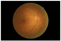 |  |  |
| Crop and resize | 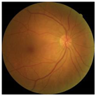 |  | 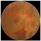 |
| CLAHE in green channel |  | 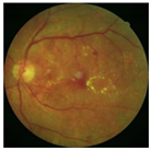 |  |
| DenseNet121 Model | Predicted Class | |||
|---|---|---|---|---|
| Normal | NPDR | PDR | ||
| Actual class | Normal | 268 | 7 | 0 |
| NPDR | 20 | 234 | 21 | |
| PDR | 15 | 25 | 235 | |
| Precision | Recall | F1-Score | |
|---|---|---|---|
| Normal | 88.4% | 97.5% | 92.7% |
| NPDR | 88% | 85.1% | 86.5% |
| PDR | 91.8% | 85.5% | 88.5% |
| Accuracy = 89.3% | |||
| Inception-ResNetV2 Model | Predicted Class | |||
|---|---|---|---|---|
| Normal | NPDR | PDR | ||
| Actual class | Normal | 270 | 3 | 2 |
| NPDR | 23 | 233 | 19 | |
| PDR | 12 | 33 | 230 | |
| Precision | Recall | F1-Score | |
|---|---|---|---|
| Normal | 88.5% | 98.2% | 93.1% |
| NPDR | 86.6% | 84.7% | 85.7% |
| PDR | 91.6% | 83.6% | 87.5% |
| Accuracy = 88.8% | |||
| Concatenate Model | Predicted Class | |||
|---|---|---|---|---|
| Normal | NPDR | PDR | ||
| Actual class | Normal | 269 | 5 | 1 |
| NPDR | 13 | 240 | 22 | |
| PDR | 10 | 27 | 238 | |
| Precision | Recall | F1-Score | |
|---|---|---|---|
| Normal | 92% | 98% | 95% |
| NPDR | 88% | 87% | 88% |
| PDR | 91% | 87% | 89% |
| Accuracy = 91% | |||
| Model | Accuracy | Macro Average Precision | Macro Average Recall | Macro Average F1-Score |
|---|---|---|---|---|
| DenseNet121 | 89.3% | 89.4% | 89.3% | 89.3% |
| Inception-ResNetV2 | 88.8% | 88.9% | 88.8% | 88.7% |
| Proposed Method | 91% | 91% | 91% | 90% |
| Method | Accuracy |
|---|---|
| Feature extraction: Gabor technique and semantic of neighbourhood colour moment features, classifier: SVM [40] | 87.61% |
| PNN and SVM [41] | PNN: 80% SVM: 90% |
| Feature extraction: PCA, classifier: SVM [42] | 86.67% |
| Feature extraction: GLCM, classifier: Fuzzy, SVM [43] | Fuzzy: 85% CNN: 90% |
| CNN (InceptionV3) [44] | 60.3% |
| CNN (AlexNet, GoogleNet, and SqueezeNet) [45] | AlexNet: 64.4% GoogleNet: 66.7% SqueezeNet: 75.6% |
| Proposed method (Concatenate model of DenseNet121 and Inception-ResNetV2 using MLP) | 91% |
Publisher’s Note: MDPI stays neutral with regard to jurisdictional claims in published maps and institutional affiliations. |
© 2021 by the authors. Licensee MDPI, Basel, Switzerland. This article is an open access article distributed under the terms and conditions of the Creative Commons Attribution (CC BY) license (https://creativecommons.org/licenses/by/4.0/).
Share and Cite
Paradisa, R.H.; Bustamam, A.; Mangunwardoyo, W.; Victor, A.A.; Yudantha, A.R.; Anki, P. Deep Feature Vectors Concatenation for Eye Disease Detection Using Fundus Image. Electronics 2022, 11, 23. https://doi.org/10.3390/electronics11010023
Paradisa RH, Bustamam A, Mangunwardoyo W, Victor AA, Yudantha AR, Anki P. Deep Feature Vectors Concatenation for Eye Disease Detection Using Fundus Image. Electronics. 2022; 11(1):23. https://doi.org/10.3390/electronics11010023
Chicago/Turabian StyleParadisa, Radifa Hilya, Alhadi Bustamam, Wibowo Mangunwardoyo, Andi Arus Victor, Anggun Rama Yudantha, and Prasnurzaki Anki. 2022. "Deep Feature Vectors Concatenation for Eye Disease Detection Using Fundus Image" Electronics 11, no. 1: 23. https://doi.org/10.3390/electronics11010023
APA StyleParadisa, R. H., Bustamam, A., Mangunwardoyo, W., Victor, A. A., Yudantha, A. R., & Anki, P. (2022). Deep Feature Vectors Concatenation for Eye Disease Detection Using Fundus Image. Electronics, 11(1), 23. https://doi.org/10.3390/electronics11010023