Pipeline Leak Detection and Estimation Using Fuzzy PID Observer

Abstract

A pipe is a ubiquitous product in the industries that is used to convey liquids, gases, or solids suspended in a liquid, e.g., a slurry, from one location to another. Both internal and external cracking can result in structural failure of the industrial piping system and possibly decrease the service life of the equipment. The chaos and complexity associated with the uncertain behaviour inherent in pipeline systems lead to difficulty in detection and localisation of leaks in real time. The timely detection of leakage is important in order to reduce the loss rate and serious environmental consequences. The objective of this paper is to propose a new leak detection method based on an autoregressive with exogenous input (ARX) Laguerre fuzzy proportional-integral-derivative (PID) observation system. The objective of this paper is to propose a new leak detection method based on an autoregressive with exogenous input (ARX) Laguerre fuzzy proportional-integral-derivative (PID) observation system. In this work, the ARX–Laguerre model has been used to generate better performance in the presence of uncertainty. According to the results, the proposed technique can detect leaks accurately and effectively.

1. Introduction

Pipelines are the safest way for transporting crude oil, petroleum products, and natural gas over long distances. Pipelines deliver clear benefits in supporting economic growth as they provide a cheaper means to transport. However, oil and gas pipelines may be significantly damaged due to internal and external defects (e.g., corrosion, dents, gouges, weld defects). Construction and operational defects of pipes can pose major risks to supplies. Pipeline safety is possible using inspection and monitoring techniques which can be either internal or external in nature.

Over the last few years, a number of technologies have been reported to monitor pipelines such as acoustic emission [1,2,3], fibre optic sensor [4,5], digital signal processing, and mass–volume balance [6]. In [7], a real-time transient modelling method has been utilised for leakage detection and localization in the pipeline systems. In [8], an extended version of a real-time transient modelling method to estimate two leaks simultaneously in a piping system is proposed. The acoustic pulse reflectometry method has been used successfully to identify damage in pipelines utilising the time domain [9].

In [10], the cepstrum analysis technique is utilised to identify leaks in pipes. In [11], a new method based on auxiliary mass spatial probing by the stationary wavelet transform is suggested to detect damage in beams. Artificial intelligence with fuzzy logic has become the most effective approach, which attracts many investigators to deeply research it [12,13,14,15,16]. It has been successfully used for leak detection. In [17], a low-cost wireless sensor system is introduced to detect of leaks in metallic piping systems. In [18,19], a neural network technique was utilized to detect the leak in a pipeline and has provided promising results. In [20], an artificial neural network was utilized to detect the leak in a pipeline such that the sound noise data were gathered through several microphones placed within a specific distance from the damaged part. The fast Fourier transform algorithm has been performed on data and supplied to a feed-forward network for making a final decision. In [11,21], a neural network technique was used for pattern recognition in oil pipe networks.

Various researchers have used observational approaches for fault diagnosis in pipes that are based on different algorithms [22,23,24]. The authors in [25] focused on leakage reconstruction in pipe systems utilising sliding mode observer. The authors in [26,27,28] focused on leakage reconstruction in pipe systems utilising a PID (proportional-integral-derivative) model and observer. In [29], a fuzzy PI observer was used to detect leaks in pipeline. In [30], a leak inspection device consisting of an adaptive Luenberger-type observer based upon a set of two-coupled partial differential equations governing the flow dynamics is proposed. To improve the input and output performance of ARX, in [26,31], the Laguerre method is applied to ARX to filter the input and output. In [27,29], a fuzzy PID observation method using the ARX–Laguerre technique is used for diagnosing fault in pipe.

The object of this paper is to develop a new technique based on autoregressive with exogenous input Laguerre (ARX–Laguerre) fuzzy PID to detect leaks in a pipe. For this aim, in the first step, the ARX–Laguerre technique is used for pipeline modelling. In the second step, the PID observer based on the ARX–Laguerre model is designed to detect leakage in the presence of uncertainties. The numerical results demonstrate that the proposed technique detects and estimates leaks accurately. The remainder part of this paper is organized as follows: in Section 2, the pipeline model equations are described using the momentum and continuity equations. The pipeline model equations based on the ARX–Laguerre technique are given in the Section 3. The proposed new technique based on ARX–Laguerre fuzzy PID observer to detect and locate leaks in a pipe is given in Section 4. The algorithm and simulation results analysis is given in Section 5. Moreover, in this section, the proposed method is compared with some other existing methods to illustrate its value. Finally, conclusions are given.

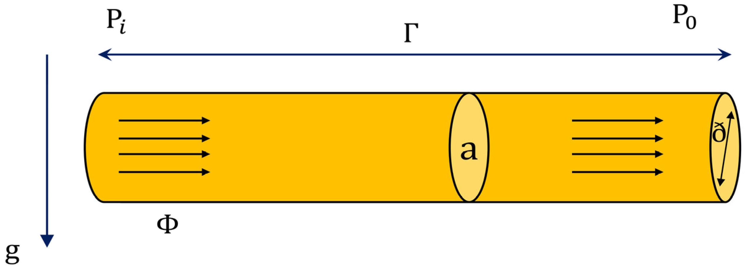
2. Pipeline Modelling

Here, we do not consider convective speed changes and compressibility effects in process lines. The mass flow rate ($m$), the length of the pipe $\left(\mathsf{\Gamma }\right)$, the flow in a pipe system $\left(\mathsf{\Phi }\right)$, the inlet pressure $\left({\wp }_i\right)$, and outlet pressure $\left({\wp }_o\right)$ at pipeline are assumed to be computable. Furthermore, the area of cross section$\left(\mathrm{a}\right)$ is fixed along the pipe. The suggested pipeline architecture is illustrated in Figure 1.

The differential equation describing the dynamic behaviour of a fluid in a duct is based on the mass, momentum, and the conservation of energy [32]. Newton’s second law of motion, when implemented to a control volume, generated the following momentum equation [32,33]:

$$\frac{\partial \upsilon }{\partial t}+\frac{1}{\rho }\frac{\partial \wp }{\partial x}+\frac{\Im }{2ð}{\upsilon }^2=0$$

(1)

If we substitute $\upsilon =\frac{\mathsf{\Phi }}{\mathrm{a}}$as well as$\wp =\rho g\mathcal{H}$ in (1) the resulting momentum equation will be:

$$\frac{\partial \mathsf{\Phi }}{a\partial t}+g\frac{\partial }{\partial x}\mathcal{H}+\frac{\Im {\mathsf{\Phi }}^2}{2ða^2}=0$$

(2)

Thus,

$$\frac{\partial \mathsf{\Phi }}{\partial t}+ag\frac{\partial }{\partial x}\mathcal{H}+\frac{\Im {\mathsf{\Phi }}^2}{2ða}=0$$

(3)

in which $\mathcal{H}$ represents the pressure head, $\mathsf{\Phi }$the rate of flow in a pipe,$x$the length of pipe, $t$ time steps, $g$ the gravity, $a$ the pipe cross-sectional area, $ð$ the inside diameter of the pipe, and $\Im$ the pipe friction factor.

Coefficient of friction is typically assumed to be constant. In general, it was found to be a function of the Reynolds number$\left(Re\right)$ and the pipe material roughness coefficient$\left(e\right)$. The Swamee–Jain equation can be used to describe the friction factor for a pipe of circular section $(ð)$ as follows [34,35]:

$$\Im ={\left(\frac{0.5}{ \ln [0.27\left(\frac{e}{ð}\right)+5.74\frac{1}{R{e}^{0.9}}]}\right)}^2$$

(4)

where $\Im$ is the pipe friction factor, $ð$ is the inside diameter of the pipe and the pipe material roughness coefficient$\left(e\right)$

Reynolds number equation is determined via the following equation [36]:

$$Re=4\frac{\rho \mathsf{\Phi }}{\pi ð\mu }=\frac{\rho \nu ð}{\mu }$$

(5)

in which $\rho$ represents the fluid density, and $\mu$ the viscosity of the flowing fluid. For ${10}^{-8}<\frac{e}{ð}<0.01$ as well as $5000<Re<{10}^8$ are provably correct.

$$\frac{\partial \wp }{\partial t}+\rho a^2\frac{\partial \nu }{\partial x}=0$$

(6)

After applying the overall mass balance as well as the Reynolds transport theorem to the control volume the continuity equation will be obtained:

$$\frac{\partial \wp }{\partial t}+\rho a^2\frac{\partial v}{\partial x}=0$$

(7)

The following equation can be acquired if we substitute the pressure head$\left(\mathcal{H}\right)$as well as the flow rate $\left(\mathsf{\Phi }\right)$ in Equation (7):

$$\frac{\partial \mathcal{H}}{\partial t}+\frac{a^2}{ga}\frac{\partial \mathsf{\Phi }}{\partial x}=0$$

(8)

in which $a$ represents the speed of the wave inside a fluid filled elastic duct. The wave velocity depends on the elastic properties of the fluid and pipe. The pressure head $\left(\mathcal{H}\right)$ and flow rate $\left(\mathsf{\Phi }\right)$ change as functions of position and time, $\mathcal{H}\left(x,t\right)$ and $\mathsf{\Phi }\left(x,t\right),$ respectively, so that $x\in \left[0,\mathsf{\Gamma }\right]$, where $\mathsf{\Gamma }$ represents the length of the duct.

Now we can create a model of the pipe applying Equations (3) and (8). These equations need to be solved; however, coming to analytical solutions is not easy. Because of this, different methods need to be used to solve these equations such as characteristics and finite difference approaches [37]. Here, the finite difference approach is implemented such that Equations (3) and (8) are discretized to obtain a system of ordinary differential equations. The considered finite difference approach discretizes the whole pipe into $N$ smaller sections [37,38]. Finite difference technique with a fixed step size$\Delta s$ is, historically, the most popular time-stepping approach. Here, we consider finite difference method because it is an easy-to-use approach and is specially designed and applied for nonlinear observer models. In this study we define it as follows:

$$\begin{gathered} \frac{\partial \mathsf{\Phi }\left(s_{i-1},t\right)}{\partial s}\approx \frac{\Delta \mathsf{\Phi }\left(s_{i-1},t\right)}{\Delta s}\approx \frac{{\mathsf{\Phi }}_i-{\mathsf{\Phi }}_{i-1}}{\Delta s} \\ \frac{\partial \mathcal{H}\left(s_{i-1},t\right)}{\partial s}\approx \frac{\Delta \mathcal{H}\left(s_{i-1},t\right)}{\Delta s}\approx \frac{{\mathcal{H}}_i-{\mathcal{H}}_{i-1}}{\Delta s} \end{gathered}$$

(9)

$\forall i=1,\cdots , n,$ in which $n$ represents the number of points of the grid, and $\Delta s=s_{i+1}-s_i$ represents the size of the $i$-section between the two successive grid points. The computational domain $s\in \left[0,\mathsf{\Gamma }\right]$ is divided up into three smaller domains,$\left\{s_k\right\}≔\left\{0,s_{leak},\mathsf{\Gamma }\right\}$, so that $s_{leak}$ indicates the location of leak; see Figure 2. The leak flow rate can be measured by ${\mathsf{\Phi }}_{leak}=C_d{a}_{leak}\sqrt{2g}\sqrt{\mathcal{H}\left(s_{leak}, t\right)}$, such that $C_d$ represents efflux coefficient, and $a_{leak}$ the cross-sectional area along the leak path. The leak flow rate can be calculated by ${\mathsf{\Phi }}_{leak}=\mathsf{\Lambda }\sqrt{\mathcal{H}\left(s_{leak}, t\right)}$, in which $\mathsf{\Lambda }=C_d{a}_{leak}\sqrt{2g}$. The behaviour of a dynamic pipeline network can be described by an ordinary differential equation system:

$$\begin{gathered} { \dot{\mathsf{\Phi }} }_1=\frac{ga}{s}\left({\mathcal{H}}_1-{\mathcal{H}}_2\right)-\frac{\Im {\mathsf{\Phi }}_1{}^2}{2ða} \\ {\dot{\mathcal{H}}}_{leak}=\frac{c^2}{gas}\left({\mathsf{\Phi }}_1-{\mathsf{\Phi }}_2-\mathsf{\Lambda }\sqrt{{\mathcal{H}}_{leak}}\right) \\ { \dot{\mathsf{\Phi }} }_2=\frac{ga}{\mathsf{\Gamma }-s}\left({\mathcal{H}}_2-{\mathcal{H}}_3\right)-\frac{\Im {\mathsf{\Phi }}_2^2}{2ða} \end{gathered}$$

(10)

Suppose that both inlet and outlet pressures, ${\mathcal{H}}_1$ and ${\mathcal{H}}_3$, respectively, are known and have been defined using external means such as a pump. The pressure ${\mathcal{H}}_2$and the inlet and outlet flow rate $({\mathsf{\Phi }}_1$ and ${\mathsf{\Phi }}_2$, respectively) of the leakage point are considered to be variables. From the continuity equation we can write:

$${\mathsf{\Phi }}_1={\mathsf{\Phi }}_{leak}+{\mathsf{\Phi }}_2$$

(11)

3. Pipeline Modelling Based on the ARX–Laguerre Technique

For many years, pipelines played a huge role in oil and gas industries, as they significantly reduce transport costs. Leakage inspection in transmission pipelines is crucially significant for safe operation. In general, there are various fault detection methods, each with different potentials; however, the selection of proper leak detection technique is difficult. This is particularly important when they deal with various types of uncertain conditions. To deal with this problem, we introduce a fuzzy ARX–Laguerre PID observer in Section 4. First, in this study, the ARX–Laguerre technique is used for pipeline modelling. In the second step, the PID observer based on the ARX–Laguerre model is designed to detect leakage in the presence of uncertainties. The proposed model-based ARX–Laguerre orthonormal method is represented by developing its coefficients associated to the flow input and flow output, Fourier coefficients, and Laguerre-based orthonormal function, as follows [23,39]:

$$M_0\left(s\right)=\sum _0^{i_a}{\lambda }_{n.a}\left(\sum _{j=1}^{\infty }{\mathcal{l}}_a\ast M_0\left(s\right)\right).x_{n.M_0}\left(s\right)+\sum _0^{i_b}{\lambda }_{n.b}\left(\sum _{j=1}^{\infty }{\mathcal{l}}_b\ast M_i\left(s\right)\right).x_{n.M_i}\left(s\right)$$

(12)

in which $M_0\left(s\right),$ $\left({\lambda }_{n.a} and {\lambda }_{n.b}\right),$ $\left(i_a,i_b\right)$ $\left({\mathcal{l}}_a, {\mathcal{l}}_b\right)$,$\ast$,$M_i\left(s\right)$, $x_{n.M_0}\left(s\right)$, and $x_{n.M_i}\left(s\right)$ represent the pipe outflow, Fourier coefficients, the order of the system, Laguerre orthonormal function, convolution product, pipe inflow, exhaust filter, and entrance filter, respectively. By expanding the ARX model on Laguerre orthonormal bases, the following state-space model can be obtained:

$$\{\begin{array}{c}M\left(s+1\right)=\left[AM\left(s\right)+B_y\left(y\left(s\right)+{\alpha }_s\left(k\right)\right)+B_u\left(u\left(s\right)+a_p\left(s\right)\right)\right]\\ y\left(s\right)={\left(S\right)}^{T}M\left(s\right)+B_s{\alpha }_s\left(s\right),\end{array}$$

(13)

in which $M\left(s\right),y\left(s\right), u\left(s\right), {\alpha }_p\left(s\right), \mathrm{and} {\alpha }_s\left(s\right)$ represent the state vector, calculated output, control input, pump defect, and sensor defect, respectively. $A, B_y, B_u, \mathrm{and} B_s, \mathrm{as} \mathrm{well} \mathrm{as} S$, represent matrices of coefficients.

4. ARX–Laguerre Fuzzy PID Observation Technique

In this section, the ARX–Laguerre fuzzy PID observation system is proposed to detect and estimate a leak in pipelines.

4.1. Modelling of Dynamic System by ARX–Laguerre

Let us consider the linear ARX state space model with disturbances illustrated by the following equation to formulate the dynamic fault detection problem:

$$\{\begin{array}{c}M\left(s+1\right)=\left[A M\left(s\right)+B_u\left(u\left(s\right)+{\alpha }_p\left(s\right)\right)\right]\\ y\left(s\right)={\left(S\right)}^{T}M\left(s\right)+B_s{\alpha }_s\left(s\right),\end{array}$$

(14)

We define the ARX model on Laguerre base as follows [31,40]:

$$\begin{gathered} y\left(k\right)=\sum _0^{N_a-1}{S}_{\left(n,p\right)}{x}_{\left(n,y\right)}\left(s\right)+\sum _0^{N_b-1}{S}_{\left(n,b\right)}{x}_{\left(n,u\right)}\left(s\right) \\ X\left(k\right)=\left[\begin{array}{cc}{x}_{\left(n,u\right)}\left(s\right)& x_{\left(n,y\right)}\left(s\right)\end{array}\right] \\ {x}_{\left(n,y\right)}\left(s\right)=L_n^a\left(k,{\xi }_p\right)\ast y\left(s\right) \\ {x}_{\left(n,u\right)}\left(s\right)=L_n^b\left(k,{\xi }_b\right)\ast u\left(s\right) \end{gathered}$$

(15)

in which $y\left(k\right), u\left(k\right), \left(K_{\left(n,p\right)},K_{\left(n,s\right)}\right), \left(N_a,N_b\right),x_{\left(n,y\right)}\left(s\right),x_{\left(n,u\right)}\left(s\right), \mathrm{and} \left(L_n^a\left(s,{\xi }_a\right),L_n^b\left(s,{\xi }_b\right)\right)$ represent the pipe outflow, pipe inflow, Fourier coefficients, exhaust filter, entrance filter, and Laguerre orthonormal function, respectively.

Using Equation (16) the following state-space model can be obtained in the presence of failures of the pump and sensor as well as disturbances:

$$\{\begin{array}{c}{M}_p\left(s+1\right)=\left[A{M}_p\left(s\right)+B_y\left(y_p\left(s\right)+{\alpha }_s\left(s\right)\right)+B_u\left(u\left(s\right)+{\alpha }_p\left(s\right)\right)\right]\\ y\left(s\right)={\left(S\right)}^T{M}_p\left(s\right)+B_s{\alpha }_s\left(s\right),\end{array}$$

(16)

The fault of the pump is calculated using the following formula:

$$\begin{array}{c}{e}_y\left(s\right)=y_p\left(s\right)-y\left(s\right)\\ e_M\left(s\right)=\left[\begin{array}{c}{x}_{p\left(n,u+{\alpha }_p\right)}\left(s\right)-x_{\left(n,u\right)}\left(s\right)\\ x_{p\left(n,y_a\right)}\left(s\right)-x_{\left(n,y\right)}\left(s\right)\end{array}\right]\end{array}$$

(17)

such that

$$x_{a\left(n,u+{\alpha }_p\right)}\left(s\right)\ne M_{\left(n,u\right)}\left(s\right)\to M_p\left(s\right)\ne M\left(s\right)\to y_p\left(s\right)\ne y\left(s\right)\to e_y\left(s\right)\ne 0$$

(18)

The fault of the sensor is calculated using the following formula:

$$\begin{array}{c}{e}_y\left(s\right)=y_p\left(s\right)-y\left(s\right)\\ e_M\left(s\right)=\left[\begin{array}{c}{M}_{p\left(n,u\right)}\left(k\right)-M_{\left(n,u\right)}\left(s\right)\\ M_{p\left(n,y_p+{\alpha }_s\right)}\left(k\right)-M_{\left(n,y\right)}\left(s\right)\end{array}\right]\end{array}$$

(19)

such that

$$M_{p\left(n,y_p+{\alpha }_s\right)}\left(s\right)\ne x_{\left(n,y\right)}\left(s\right)\to M_p\left(s\right)\ne M\left(s\right)\to y_p\left(s\right)\ne y\left(s\right)\to e_y\left(S\right)\ne 0.$$

(20)

4.2. Fault Diagnosis

In this study, the ARX–Laguerre fuzzy PID observation system is proposed to identify pump and sensor defects in pipes. We define the proposed technique by the following formulas in the presence of failures of the pump and sensor in the pipe:

$$\{\begin{array}{c}\begin{array}{c}\widehat{M}\left(s+1\right)=A\widehat{M}\left(s\right)+B_y\left(\widehat{y}\left(s\right)+{\widehat{\alpha }}_s\left(s\right)\right)+B_y\left(u\left(s\right)+{\widehat{\alpha }}_p\left(s\right)\right)+K_{p}e\left(s\right)\\ e_s\left(s\right)=\left(q_s\left(s\right)-{\widehat{q}}_s\left(s\right)\right)\\ e_p\left(s\right)=\left(w_p\left(s\right)-{\widehat{w}}_p\left(s\right)\right)\end{array}\\ {\widehat{\alpha }}_p\left(s+1\right)={\widehat{\alpha }}_p\left(s\right)+K_{ip}{e}_p\left(s\right)+K_{d_p}\left(e_p\left(s+1\right)+e_p\left(s\right)+e_p\left(s-1\right)\right)\\ \begin{array}{c}{\widehat{\alpha }}_s\left(s+1\right)={\widehat{\alpha }}_s\left(s\right)+K_{is}{e}_s\left(s\right)+K_{d_s}\left(e_s\left(s+1\right)+e_s\left(s\right)+e_s\left(s-1\right)\right)\\ \widehat{y}\left(s+1\right)={\left(S\right)}^T\widehat{M}\left(s+1\right)+{\beta }_s{\widehat{\alpha }}_s\left(s\right)\end{array}\end{array}$$

(21)

where $\widehat{M}\left(s\right)$ represents the state vector, ${\alpha }_p\left(s\right)$ pump defect, ${\alpha }_s\left(s\right)$ sensor defect, and $\widehat{y}\left(s\right)$ the output of the system, and $A, B_y, B_u, \mathrm{and} B_s, \mathrm{as} \mathrm{well} \mathrm{as} S$, represent matrices of coefficients. In accordance with Equation (21), in this paper, we particularly study three main cases and types of faults in pipe.

Case 1: In case ${\alpha }_p\ne 0, {\alpha }_s=0$, and ${\widehat{\alpha }}_p\left(s\right)\ne {\alpha }_p\left(s\right)$, we have:

$$\begin{array}{c}\left(y\left(s+1\right)-\widehat{y}\left(s+1\right)\ne 0\right)\& \left(M\left(s+1\right)-\widehat{M}\left(s+1\right)\right)\ne 0 ⟹ \\ \begin{array}{c}{\left[\begin{array}{cc}{M}_1^T\left(s+1\right)& M_2^T\left(s+1\right)\end{array}\right]}^T-{\left[\begin{array}{cc}{\widehat{M}}_1^T\left(s+1\right)& {\widehat{M}}_{2,{\alpha }_p}^T\left(s+1\right)\end{array}\right]}^T\ne 0⟹ \\ \{\begin{array}{c}{M}_{\left(n,u\right)}\left(s\right)-{\widehat{M}}_{\left(n,u+{\alpha }_p\right)}\left(s\right)\ne 0\\ M_{\left(n,y\right)}\left(s\right)-{\widehat{M}}_{\left(n,y\right)}\left(s\right)\ne 0\end{array}\end{array}\end{array}$$

(22)

In case ${\alpha }_p\ne 0, {\alpha }_s=0$, and ${\widehat{\alpha }}_p\left(s\right)={\alpha }_p\left(s\right)$, we have:

$$\begin{array}{c}\left(y\left(s+1\right)-\widehat{y}\left(s+1\right)=0\right)\& \left(M\left(s+1\right)-\widehat{M}\left(s+1\right)\right)\ne 0 ⟹ \\ \begin{array}{c}{\left[\begin{array}{cc}{M}_1^T\left(s+1\right)& M_2^T\left(s+1\right)\end{array}\right]}^T-{\left[\begin{array}{cc}{\widehat{M}}_1^T\left(s+1\right)& {\widehat{M}}_{2,{\alpha }_p}^T\left(s+1\right)\end{array}\right]}^T\ne 0⟹ \\ \{\begin{array}{c}{M}_{\left(n,u\right)}\left(s\right)-{\widehat{M}}_{\left(n,u+{\alpha }_p\right)}\left(s\right)\ne 0\\ M_{\left(n,y\right)}\left(s\right)-{\widehat{M}}_{\left(n,y\right)}\left(s\right)=0\end{array}\end{array}\end{array}$$

(23)

In accordance with Equations (22) and (23), in case the error related to ARX–Laguerre fuzzy PID technique is close to zero, the detection rate of defect is very high.

The following formula can be defined for fault in the pump:

$${\widehat{\alpha }}_p={\alpha }_q\to q_p-{\widehat{q}}_p\cong 0 \& w-\widehat{w}\ne 0\to r=w-\widehat{w}$$

(24)

Case 2: In case ${\alpha }_s\ne 0, {\alpha }_p=0$, and ${\widehat{\alpha }}_s\left(s\right)\ne {\alpha }_s\left(s\right)$, we have:

$$\begin{array}{c}\left(y\left(s+1\right)-\widehat{y}\left(s+1\right)\ne 0\right)\& \left(M\left(s+1\right)-\widehat{M}\left(s+1\right)\right)\ne 0 ⟹ \\ \begin{array}{c}{\left[\begin{array}{cc}{M}_1^T\left(s+1\right)& M_2^T\left(s+1\right)\end{array}\right]}^T-{\left[\begin{array}{cc}{\widehat{M}}_1^T\left(s+1\right)& {\widehat{M}}_{2,{\alpha }_p}^T\left(s+1\right)\end{array}\right]}^T\ne 0⟹ \\ \{\begin{array}{c}{M}_{\left(n,u\right)}\left(s\right)-{\widehat{M}}_{\left(n,u\right)}\left(s\right)\ne 0\\ M_{\left(n,y\right)}\left(s\right)-{\widehat{M}}_{\left(n,y+{\alpha }_s\right)}\left(s\right)\ne 0\end{array}\end{array}\end{array}$$

(25)

In case ${\alpha }_s\ne 0, {\alpha }_p=0$, and ${\widehat{\alpha }}_s\left(s\right)={\alpha }_s\left(s\right)$, we have:

$$\begin{array}{c}\left(y\left(s+1\right)-\widehat{y}\left(s+1\right)=0\right)\& \left(M\left(s+1\right)-\widehat{M}\left(s+1\right)\right)\ne 0 ⟹ \\ \begin{array}{c}{\left[\begin{array}{cc}{M}_1^T\left(s+1\right)& M_2^T\left(s+1\right)\end{array}\right]}^T-{\left[\begin{array}{cc}{\widehat{M}}_1^T\left(s+1\right)& {\widehat{M}}_{2,{\alpha }_p}^T\left(s+1\right)\end{array}\right]}^T\ne 0⟹ \\ \{\begin{array}{c}{M}_{\left(n,u\right)}\left(s\right)-{\widehat{M}}_{\left(n,u\right)}\left(s\right)=0\\ x_{\left(n,y\right)}\left(s\right)-{\widehat{x}}_{\left(n,y+{\alpha }_s\right)}\left(s\right)\ne 0\end{array}\end{array}\end{array}$$

(26)

In accordance with Equations (25) and (26), the ARX–Laguerre fuzzy PID has a significant influence on the efficiency of sensor defect detection in a duct.

The following formula can be defined for fault in sensor:

$${\widehat{\alpha }}_s={\alpha }_s\to w-\widehat{w}\cong 0 \& q_p-{\widehat{q}}_p\ne 0\to r=q_p-{\widehat{q}}_p$$

(27)

Case 3: In case ${\alpha }_s\ne 0, {\alpha }_p=0$, ${\widehat{\alpha }}_s\left(s\right)\ne {\alpha }_s\left(s\right)$, and ${\widehat{\alpha }}_p\left(s\right)\ne {\alpha }_p\left(s\right)$ we have:

$$\begin{array}{c}\left(y\left(s+1\right)-\widehat{y}\left(s+1\right)\ne 0\right)\& \left(M\left(s+1\right)-\widehat{M}\left(s+1\right)\right)\ne 0 ⟹ \\ \begin{array}{c}{\left[\begin{array}{cc}{M}_1^T\left(s+1\right)& M_2^T\left(s+1\right)\end{array}\right]}^T-{\left[\begin{array}{cc}{\widehat{M}}_{1,{\alpha }_s}^T\left(s+1\right)& {\widehat{M}}_2^T\left(s+1\right)\end{array}\right]}^T\ne 0⟹ \\ \{\begin{array}{c}{M}_{\left(n,u\right)}\left(s\right)-{\widehat{M}}_{\left(n,u+{\alpha }_p\right)}\left(s\right)\ne 0\\ M_{\left(n,y\right)}\left(s\right)-{\widehat{M}}_{\left(n,y+{\alpha }_s\right)}\left(s\right)\ne 0\end{array}\end{array}\end{array}$$

(28)

In case ${\alpha }_s\ne 0, {\alpha }_p=0$, and ${\widehat{\alpha }}_s\left(s\right)={\alpha }_s\left(s\right)$, we have:

$$\begin{array}{c}\left(y\left(s+1\right)-\widehat{y}\left(s+1\right)\ne 0\right)\& \left(M\left(s+1\right)-\widehat{M}\left(s+1\right)\right)\ne 0 ⟹ \\ \begin{array}{c}{\left[\begin{array}{cc}{M}_1^T\left(s+1\right)& M_2^T\left(s+1\right)\end{array}\right]}^T-{\left[\begin{array}{cc}{\widehat{M}}_1^T\left(s+1\right)& {\widehat{M}}_{2,{\alpha }_p}^T\left(s+1\right)\end{array}\right]}^T\ne 0⟹ \\ \{\begin{array}{c}{M}_{\left(n,u\right)}\left(s\right)-{\widehat{M}}_{\left(n,u+{\alpha }_p\right)}\left(s\right)\ne 0\\ M_{\left(n,y\right)}\left(s\right)-{\widehat{M}}_{\left(n,y+{\alpha }_s\right)}\left(s\right)\ne 0\end{array}\end{array}\end{array}$$

(29)

In accordance with Equation (29), in case the pipe includes sensor and pump failures, the signals received from pump and joint variable can identify the defects. Signal sensor and pump faults are:

$${\widehat{\alpha }}_p={\alpha }_p\& {\widehat{\alpha }}_s={\alpha }_s\to r_1=w-\widehat{w}\gg 0 \& r_2=q_p-{\widehat{q}}_p\gg 0$$

(30)

To increase the signal estimation accuracy and to modify the performance of fault estimation of the ARX–Laguerre PID technique, optimal fuzzy observer coefficients, $K_{p_p},K_{i_p},K_{d_p},K_{p_s},K_{i_s}$ and $K_{d_s}$, are applied, which are defined as follows:

$$\begin{array}{c}{K}_{i_p}=\frac{K_{p_p}}{T_{i_p}}, K_{d_p}=K_{p_p}.T_{d_p}\\ K_{i_s}=\frac{K_{p_s}}{T_{i_s}}, K_{d_s}=K_{p_s}.T_{d_s}\end{array}$$

(31)

where $T_{i_p}, T_{i_s},T_{d_p}$, and $T_{d_s},$ represent the integral gain for pump failure, the integral gain for sensor failure, the derivative gain for pump failure, and the derivative gain for sensor failure, respectively. Following Equation (29), we have:

$$\begin{array}{c}{\beta }_p=\frac{T_{i_p}}{T_{i_p}}, K_{ip}=\frac{{\left(K_{p_p}\right)}^2}{{\beta }_p{K}_{d_p}}\\ {\beta }_s=\frac{T_{i_s}}{T_{i_s}}, K_{i_s}=\frac{{\left(K_{p_s}\right)}^2}{{\beta }_s{K}_{d_s}}\end{array}$$

(32)

Normalization of the above equation can be performed by the formula described below:

$$\begin{gathered} K{\text{'}}_{p_p}=\frac{K_{p_p}-K_{p_p\left(min\right)}}{K_{p_p\left(max\right)}-K_{p_p\left(min\right)}}\in \left[0,1\right], K{\text{'}}_{p_p}=\frac{K_{d_p}-K_{d_p\left(min\right)}}{K_{p_p\left(max\right)}-K_{p_p\left(min\right)}}\in \left[0,1\right],2\le {\beta }_p\le 5 \\ K{\text{'}}_{p_s}=\frac{K_{p_s}-K_{p_s\left(min\right)}}{K_{p_s\left(max\right)}-K_{p_s\left(min\right)}}\in \left[0,1\right], K{\text{'}}_{d_s}=\frac{K_{d_s}-K_{d_s\left(min\right)}}{K_{d_s\left(max\right)}-K_{d_s\left(min\right)}}\in \left[0,1\right],2\le {\beta }_s\le 5 \end{gathered}$$

(33)

such that $\beta =\frac{{\sum }_i^{}\alpha \left(x_i\right) · x_i }{{\sum }_i^{}\alpha \left(x_i\right)}$ represents a membership function.

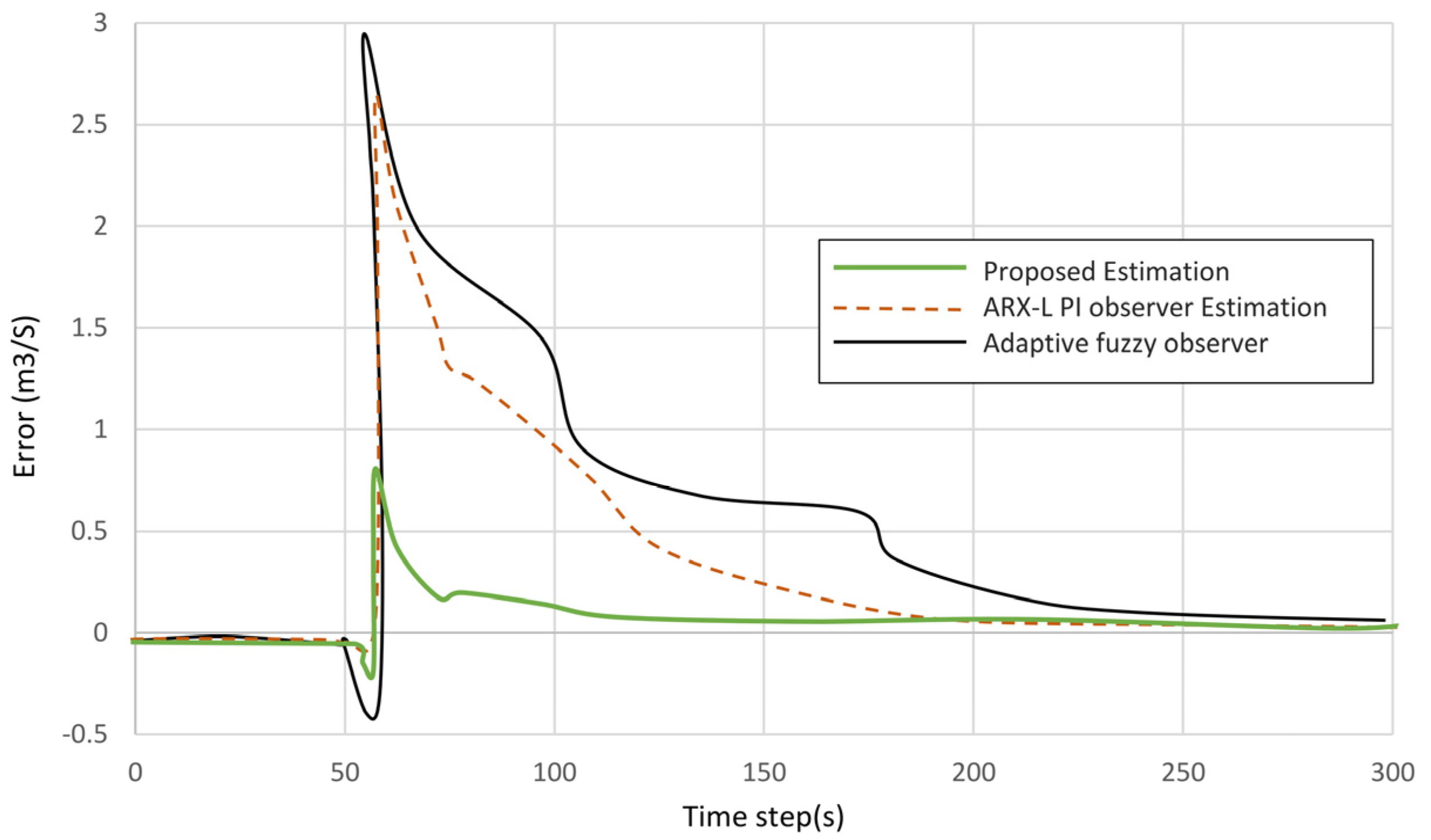
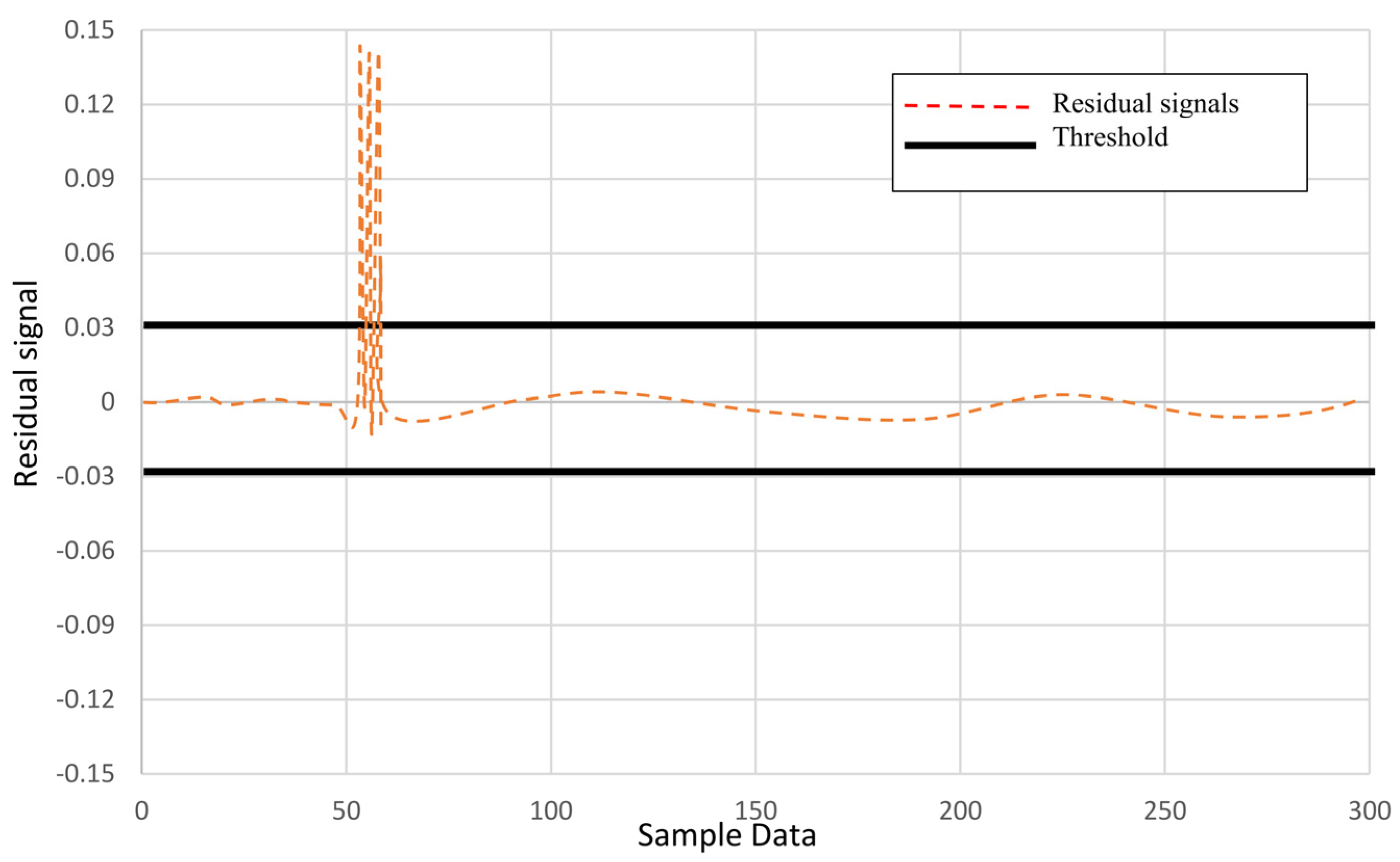
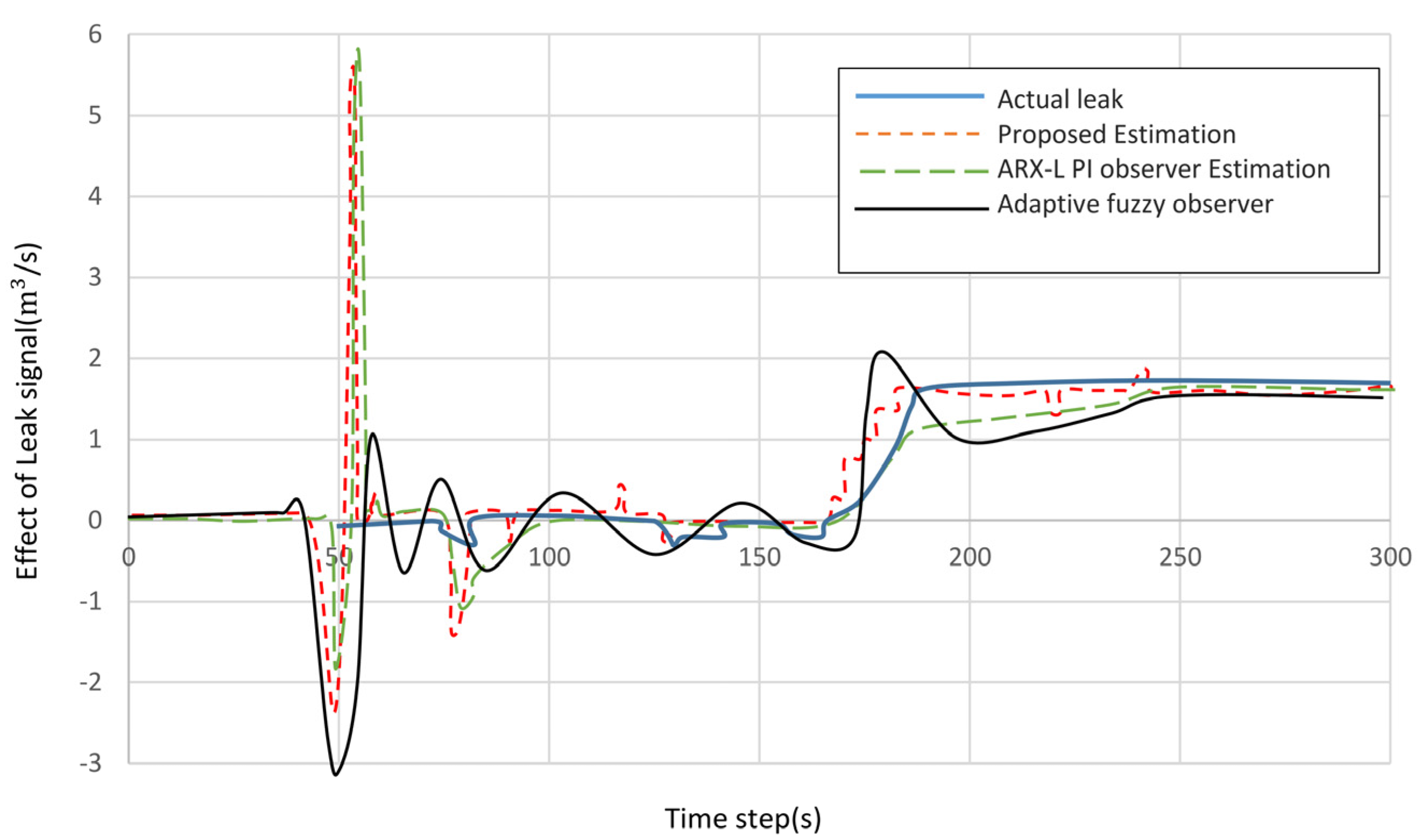
5. Simulation Results

In this section, we evaluate our proposed technique on a pipe model under the leak condition in the presence of failures of the pump and sensor in the pipe. In order to check the efficiency of the proposed ARX–Laguerre fuzzy PID observation technique for fault detection in the pipe, we consider two cases, pipe with fault and under no-fault conditions.

Pipe under no-fault condition. In this case, the duct functions under optimal circumstances and performs well. The input–output signals of the pipe model in a healthy state can be computed as follows:

$$\begin{array}{c}r\left(w\right)=w-\widehat{w}\to r\left(w\right)=w-\left(w_{Observer}+{\alpha }_p\right)\to r\left(w\right)=w-\left(w_{Observer}+0\right)\cong 0\\ r\left(\varphi \right)=\varphi -\widehat{\varphi }\to r\left(\varphi \right)=\varphi -\left({\varphi }_{Observer}+{\alpha }_s\right)\to r\left(\varphi \right)=\varphi -\left({\varphi }_{Observer}+0\right)\cong 0\end{array}$$

(34)

The sensor signal for the pipe under no-fault condition and no noise impact is shown in Figure 3. The pump signal for the pipe under no-fault condition and no noise impact is shown in Figure 4.

For a healthy system, the pump and sensor faults can be described as follows:

$$\begin{array}{c}Faul{t}_{pump}={\alpha }_p\left(t-t_0\right)=\{\begin{array}{c}0, t<t_p\\ {\alpha }_p, t>t_p\end{array}\\ Faul{t}_{sensor}={\alpha }_s\left(t-t_0\right)=\{\begin{array}{c}0, t<t_s\\ {\alpha }_s, t>t_s\end{array}\end{array}$$

(35)

The effectiveness of the proposed technique for fault estimation under no-fault condition is shown Figure 5. As can be observed from Figure 5, the proposed method is more effective than the ARX–Laguerre PI observer [41] and the adaptive fuzzy observer [42]. The error between the predicted output and the expected output based on the proposed technique under no-fault condition is shown in Figure 6. It can be seen that the proposed method yields more accurate results compared with ARX–Laguerre PI observer [41] and the adaptive fuzzy observer [42].

Pipe under fault condition. In this case, the duct functions under faulty circumstances. The duct has two kinds of defects simultaneously, the sensor defect and the pump defect.

The input–output signals from sensor and pump in the pipe with a fault state can be computed as follows:

$$\begin{array}{c}r\left(w\right)=w-\widehat{w}\to r\left(w\right)=w-\left(w_{Observer}+{\alpha }_p\right)\gg 0\\ r\left(\varphi \right)=\varphi -\widehat{\varphi }\to r\left(\varphi \right)=\varphi -\left({\varphi }_{Observer}+{\alpha }_s\right)\gg 0\end{array}$$

(36)

where

$$\begin{array}{c}{w}_1{}_{{\alpha }_p}\left(m\right)=\{\begin{array}{c}55, 10\le t\le 25\\ 0, otherwise\end{array}\\ {\varphi }_1{}_{{\alpha }_s}\left(m\right)=\{\begin{array}{c}0.6, 10\le t\le 25\\ 0, otherwise\end{array}\end{array}$$

(37)

The pump signal for the pipe under fault condition and no noise impact is shown in Figure 7. The sensor signal for the pipe under fault condition is shown in Figure 8.

The effectiveness of the proposed technique for fault estimation under fault condition is shown Figure 9. As can be observed from Figure 9, the proposed method is more effective than the ARX–Laguerre PI observer [41] and the adaptive fuzzy observer [42]. The error between the predicted output and the expected output based on the proposed technique under fault condition is shown in Figure 10. It can be seen that the proposed method yields more accurate results compared with ARX–Laguerre PI observer [41] and the adaptive fuzzy observer [42]. Furthermore, the delay for the proposed method to fault detection in both Figure 9 and Figure 10 is less than the other methods.

The effectiveness of the proposed technique for fault estimation at leakage point is shown in Figure 11. It can be seen from this figure that our proposed method detects fault in less time in comparison with ARX–Laguerre PI observer [41] and the adaptive fuzzy observer [42].

6. Conclusions

The task of precise defect detection in the pipeline system is a formidable challenge due to the uncertainties in leak signal. To better deal with uncertainties in the leak signal, in this paper, an ARX–Laguerre PID-observer is introduced to perform fault diagnosis in the pipeline system. First, in this study, the ARX–Laguerre technique was used for pipeline modelling. In the second step, the PID observer based on the ARX–Laguerre model was designed to detect leakage in the presence of uncertainties. The performance of the proposed algorithm was tested in numerical simulations. According to the results, the proposed technique can accurately locate the leakage point. Despite the high accuracy of the proposed fault diagnosis method, it has a disadvantage of large extensive computation. In the future, the proposed observation method will be used to enhance the performance of fault diagnosis when the uncertainties are in the form of Z-numbers.

References

1. Meng, L.; Yuxing, L.; Wuchang, W.; Juntao, F. Experimental study on leak detection and location for gas pipeline based on acoustic method. J. Loss Prev. Process Ind. 2012, 25, 90–102. [Google Scholar] [CrossRef]
2. Jin, H.; Zhang, L.; Liang, W.; Ding, Q. Integrated leakage detection and localization model for gas pipelines based on the acoustic wave method. J. Loss Prev. Process Ind. 2014, 27, 74–88. [Google Scholar] [CrossRef]
3. Mahmutoglu, Y.; Turk, K. A passive acoustic based system to locate leak hole in underwater natural gas pipelines. Digital Signal Process. 2018, 76, 59–65. [Google Scholar] [CrossRef]
4. Lim, K.; Wong, L.; Chiu, W.K.; Kodikara, J. Distributed fiber optic sensors for monitoring pressure and stiffness changes in out-of-round pipes. Struct. Control Health Monitor. 2016, 23, 303–314. [Google Scholar] [CrossRef]
5. Jia, Z.; Ren, L.; Li, H.; Sun, W. Pipeline leak localization based on FBG hoop strain sensors combined with BP neural network. Appl. Sci. 2018, 8, 146. [Google Scholar] [CrossRef] [Green Version]
6. Wan, J.; Yu, Y.; Wu, Y.; Feng, R.; Yu, N. Hierarchical leak detection and localization method in natural gas pipeline monitoring sensor networks. Sensors 2012, 12, 189–214. [Google Scholar] [CrossRef] [Green Version]
7. Billmann, L.; Isermann, R. Leak detection methods for pipelines. IFAC Proc. Vol. 1984, 17, 1813–1818. [Google Scholar] [CrossRef]
8. Verde, C. Minimal order nonlinear observer for leak detection. J. Dyn. Syst. Meas. Control 2004, 126, 467–472. [Google Scholar] [CrossRef]
9. Sharp, D.; Campbell, D. Leak detection in pipes using acoustic pulse reflectometry. Acta Acust. United Acust. 1997, 83, 560–566. [Google Scholar]
10. Taghvaei, M.; Beck, S.; Staszewski, W. Leak detection in pipelines using cepstrum analysis. Measur. Sci. Technol. 2006, 17, 367. [Google Scholar] [CrossRef] [Green Version]
11. Zhao, J.; Li, D.; Qi, H.; Sun, F.; An, R. The fault diagnosis method of pipeline leakage based on neural network. In Proceedings of the 2010 International Conference on Computer, Mechatronics, Control and Electronic Engineering, Changchun, China, 24–26 August 2010; Volume 1, pp. 322–325. [Google Scholar]
12. Jafari, R.; Razvarz, S.; Gegov, A. Applications of Z-Numbers and Neural Networks in Engineering. In Science and Information Conference; Springer: Berlin/Heidelberg, Germany, 2020; pp. 12–25. [Google Scholar]
13. Jafari, R.; Razvarz, S.; Gegov, A. End-to-end memory networks: A survey. In Science and Information Conference; Springer: Berlin/Heidelberg, Germany, 2020; pp. 291–300. [Google Scholar]
14. Jafari, R.; Razvarz, S.; Gegov, A. A novel technique for solving fully fuzzy nonlinear systems based on neural networks. Vietnam J. Comput. Sci. 2020, 7, 93–107. [Google Scholar] [CrossRef] [Green Version]
15. Jafari, R.; Contreras, M.A.; Yu, W.; Gegov, A. Applications of Fuzzy Logic, Artificial Neural Network and Neuro-Fuzzy in Industrial Engineering. In Latin American Symposium on Industrial and Robotic Systems; Springer: Berlin/Heidelberg, Germany, 2019; pp. 9–14. [Google Scholar]
16. Razvarz, S.; Hernández-Rodríguez, F.; Jafari, R.; Gegov, A. Foundation of Z-Numbers and Engineering Applications. In Latin American Symposium on Industrial and Robotic Systems; Springer: Berlin/Heidelberg, Germany, 2019; pp. 15–24. [Google Scholar]
17. Christos, S.C.; Fotis, G.; Nektarios, G.; Dimitris, R.; Areti, P.; Dimitrios, S. Autonomous low-cost Wireless Sensor platform for Leakage Detection in Oil and Gas Pipes. In Proceedings of the 2021 10th International Conference on Modern Circuits and Systems Technologies (MOCAST), Thessaloniki, Greece, 5–7 July 2021; pp. 1–4. [Google Scholar]
18. Belsito, S.; Lombardi, P.; Andreussi, P.; Banerjee, S. Leak detection in liquefied gas pipelines by artificial neural networks. AIChE J. 1998, 44, 2675–2688. [Google Scholar] [CrossRef]
19. Ferraz, I.M.N.; Garcia, A.C.; Bernardini, F.V.C. Artificial neural networks ensemble used for pipeline leak detection systems. Int. Pipeline Conf. 2008, 48579, 739–747. [Google Scholar]
20. Shibata, A.; Konishi, M.; Abe, Y.; Hasegawa, R.; Watanabe, M.; Kamijo, H. Neuro based classification of gas leakage sounds in pipeline. In Proceedings of the 2009 International Conference on Networking, Sensing and Control, Okayama, Japan, 26–29 March 2009; pp. 298–302. [Google Scholar]
21. Kim, K.-H.; Lee, H.-S.; Jeong, H.-M.; Kim, H.-S.; Park, J.-H. A Study on Fault Diagnosis of Boiler Tube Leakage based on Neural Network using Data Mining Technique in the Thermal Power Plant. Trans. Korean Inst. Electr. Eng. 2017, 66, 1445–1453. [Google Scholar]
22. Gao, Z.; Cecati, C.; Ding, S.X. A survey of fault diagnosis and fault-tolerant techniques—Part I: Fault diagnosis with model-based and signal-based approaches. IEEE Trans. Ind. Electron. 2015, 62, 3757–3767. [Google Scholar] [CrossRef] [Green Version]
23. Piltan, F.; Kim, J.-M. Bearing fault diagnosis by a robust higher-order super-twisting sliding mode observer. Sensors 2018, 18, 1128. [Google Scholar] [CrossRef] [Green Version]
24. Gao, Z.; Ding, S.X.; Cecati, C. Real-time fault diagnosis and fault-tolerant control. IEEE Trans. Ind. Electron. 2015, 62, 3752–3756. [Google Scholar] [CrossRef] [Green Version]
25. Angulo, M.T.; Verde, C. Second-order sliding mode algorithms for the reconstruction of leaks. In Proceedings of the 2013 Conference on Control and Fault-Tolerant Systems (SysTol), Nice, France, 9–11 October 2013; pp. 566–571. [Google Scholar]
26. Wu, Q.; Saif, M. Robust fault diagnosis for a satellite large angle attitude system using an iterative neuron PID (INPID) observer. In Proceedings of the 2006 American Control Conference, Minneapolis, MN, USA, 14–16 June 2006; p. 6. [Google Scholar]
27. Piltan, F.; Sohaib, M.; Kim, J.-M. Fault diagnosis of a robot manipulator based on an ARX-laguerre fuzzy PID observer. In Proceedings of the International Conference on Robot Intelligence Technology and Applications, Daejeon, Korea, 16–17 December 2017; pp. 393–407. [Google Scholar]
28. Wu, A.-G.; Duan, G.-R.; Fu, Y.-M. Generalized PID observer design for descriptor linear systems. IEEE Trans. Syst. Man Cybern. Part B (Cybern.) 2007, 37, 1390–1395. [Google Scholar] [CrossRef]
29. Piltan, F.; Kim, J.-M. Pipeline Leak Detection and Estimation Using Fuzzy-Based PI Observer. In Proceedings of the International Conference on Intelligent and Fuzzy Systems, Istanbul, Turkey, 21–23 July 2019; pp. 1122–1129. [Google Scholar]
30. Aamo, O.M.; Smyshlyaev, A.; Krstic, M.; Foss, B.A. Output feedback boundary control of a Ginzburg–Landau model of vortex shedding. IEEE Trans. Autom. Control 2007, 52, 742–748. [Google Scholar] [CrossRef]
31. Bouzrara, K.; Garna, T.; Ragot, J.; Messaoud, H. Online identification of the ARX model expansion on Laguerre orthonormal bases with filters on model input and output. Int. J. Control 2013, 86, 369–385. [Google Scholar] [CrossRef]
32. Cebeci, T.; Bradshaw, P. Momentum Transfer in Boundary Layers; McGraw-Hill Book Co.: New York, NY, USA, 1977. [Google Scholar]
33. Hafeez, H.Y.; Ndikilar, C.E. 4.1 The continuity equation. In Applications of Heat, Mass and Fluid Boundary Layers; Woodhead Publishing: Sawston, UK, 2020; p. 67. [Google Scholar]
34. Swamee, P.K.; Swamee, N. Full-range pipe-flow equations. J. Hydraul. Res. 2007, 45, 841–843. [Google Scholar] [CrossRef]
35. Assunção, G.S.C.; Marcelin, D.; Filho, J.C.v.; Schiozer, D.J.; de Castro, M.S. Friction Factor Equations Accuracy for Single and Two-Phase Flows. In International Conference on Offshore Mechanics and Arctic Engineering; American Society of Mechanical Engineers: New York, NY, USA, 2020; Volume 84430, p. V011T11A043. [Google Scholar]
36. Rott, N. Note on the history of the Reynolds number. Annu. Rev. Fluid Mech. 1990, 22, 1–12. [Google Scholar] [CrossRef]
37. Tomé, M.; Mangiavacchi, N.; Cuminato, J.; Castelo, A.; McKee, S. A finite difference technique for simulating unsteady viscoelastic free surface flows. J. Non-Newton. Fluid Mech. 2002, 106, 61–106. [Google Scholar] [CrossRef]
38. Wang, X.; Wildman, R.A.; Weile, D.S.; Monk, P. A finite difference delay modeling approach to the discretization of the time domain integral equations of electromagnetics. IEEE Trans. Antennas Propag. 2008, 56, 2442–2452. [Google Scholar] [CrossRef]
39. Piltan, F.; Kim, J.-M. Advanced fuzzy-based leak detection and size estimation for pipelines. J. Intell. Fuzzy Syst. 2020, 38, 947–961. [Google Scholar] [CrossRef]
40. Kim, J.H.; Kim, K.S.; Sim, M.S.; Han, K.H.; Ko, B.S. An application of fuzzy logic to control the refrigerant distribution for the multi-type air conditioner. In Proceedings of the FUZZ-IEEE’99. 1999 IEEE International Fuzzy Systems. Conference Proceedings (Cat. No. 99CH36315), Seoul, Korea, 22–25 August 1999; Volume 3, pp. 1350–1354. [Google Scholar]
41. Najeh, T.; Njima, C.B.; Garna, T.; Ragot, J. Input fault detection and estimation using PI observer based on the ARX-Laguerre model. Int. J. Adv. Manuf. Technol. 2017, 90, 1317–1336. [Google Scholar] [CrossRef] [Green Version]
42. Tong, S.; Li, Y.; Li, Y.; Liu, Y. Observer-based adaptive fuzzy backstepping control for a class of stochastic nonlinear strict-feedback systems. IEEE Trans. Syst. Man Cybern. Part B (Cybern.) 2011, 41, 1693–1704. [Google Scholar] [CrossRef]
Figure 1. The suggested pipeline architecture.
Electronics 11 00152 g001
Figure 2. The suggested pipeline architecture.
Electronics 11 00152 g002
Figure 3. The sensor signal for the pipe under no-fault condition.
Electronics 11 00152 g003
Figure 4. The pump signal for the pipe under no-fault condition.
Electronics 11 00152 g004
Figure 5. The effectiveness of the proposed technique for fault estimation under no-fault condition.
Electronics 11 00152 g005
Figure 6. The error between the predicted output and the expected output based on the proposed technique under no-fault condition.
Electronics 11 00152 g006
Figure 7. The pump signal for the pipe under fault condition.
Electronics 11 00152 g007
Figure 8. The sensor signal for the pipe under fault condition.
Electronics 11 00152 g008
Figure 9. The effectiveness of the proposed technique for fault estimation under fault condition.
Electronics 11 00152 g009
Figure 10. The error between the predicted output and the expected output based on the proposed technique under fault condition.
Electronics 11 00152 g010
Figure 11. The effectiveness of the proposed technique for fault estimation at leakage point in pipe.
Electronics 11 00152 g011
Publisher’s Note: MDPI stays neutral with regard to jurisdictional claims in published maps and institutional affiliations.