Article

Enhanced Millimeter-Wave 3-D Imaging via Complex-Valued Fully Convolutional Neural Network

1
Beijing Key Laboratory of Millimeter-Wave and Terahertz Wave Technology, Beijing Institute of Technology, Beijing 100081, China
2
First Research Institute of the Ministry of Public Security of PRC, Beijing 100048, China
*
Author to whom correspondence should be addressed.
Electronics 2022, 11(1), 147; https://doi.org/10.3390/electronics11010147
Submission received: 28 November 2021 / Revised: 30 December 2021 / Accepted: 2 January 2022 / Published: 4 January 2022
(This article belongs to the Section Microwave and Wireless Communications)

Abstract

:
To solve the problems of high computational complexity and unstable image quality inherent in the compressive sensing (CS) method, we propose a complex-valued fully convolutional neural network (CVFCNN)-based method for near-field enhanced millimeter-wave (MMW) three-dimensional (3-D) imaging. A generalized form of the complex parametric rectified linear unit (CPReLU) activation function with independent and learnable parameters is presented to improve the performance of CVFCNN. The CVFCNN structure is designed, and the formulas of the complex-valued back-propagation algorithm are derived in detail, in response to the lack of a machine learning library for a complex-valued neural network (CVNN). Compared with a real-valued fully convolutional neural network (RVFCNN), the proposed CVFCNN offers better performance while needing fewer parameters. In addition, it outperforms the CVFCNN that was used in radar imaging with different activation functions. Numerical simulations and experiments are provided to verify the efficacy of the proposed network, in comparison with state-of-the-art networks and the CS method for enhanced MMW imaging.

1. Introduction

Millimeter-wave (MMW) imaging is widely applied in remote sensing [1,2], indoor target tracking [3], concealed weapons detection [4,5], and so on. It offers high spatial resolutions of the target under test, even behind some kind of barrier. In the past few decades, the regularized iterative methods, especially compressive sensing (CS)-based methods [6,7,8], have been widely employed to improve the image quality. In most cases, solving such ill-posed inverse problems leads to high computational complexity and unstable recovered results. Thus, the parameters of the CS method need to be carefully selected.
In recent years, deep learning methods have received much attention in many fields, such as radar monitoring [9,10], hand-gesture recognition [11,12], and radar imaging [13,14]. The network parameters were optimized in the training stage, which was time-consuming. However, when it comes to the testing stage, the processing of the network is usually fast and efficient.
In [13,14], a convolutional neural network (CNN) was employed for enhanced radar imaging. It can achieve better image quality than those achieved using Fourier methods. The undersampling scenario was approached using CNN in [15,16,17], where the initial radar imaging results were enhanced by CNN. A trained CNN-based method was proposed in [18] to realize moving-target refocusing and residual clutter elimination for ground moving-target imaging with synthetic aperture radar (SAR). The authors of [19] proposed a novel shuffle-generative adversarial network (GAN) using the autoencoder separation method to separate moving and stationary targets in SAR imagery. In [20], a three-stage approach was presented for ground moving-target indications (GMTI) in video SAR based on machine learning algorithms. In order to achieve super-resolution with a small amount of data, the image was restored through U-net and the resolution was further improved by a CS algorithm [21]. The authors of [22] proposed a deep learning method for three-dimensional (3-D) reconstruction and imaging via MMW radar. It generates two-dimensional (2-D) depth maps from the original data, and then generates a 3-D point cloud from the depth maps. In [23], the authors introduced a system for MMW-enhanced imaging through fog, which recovers high-resolution 2-D depth maps of cars from raw low-resolution MMW 3-D images with a GAN architecture. Most deep learning methods are based on the real-valued neural network (RVNN), since it is easy to construct a network using the popular real-valued machine-learning library. They do not follow the calculation rules of complex numbers and the phase of reconstruction results is usually not preserved. However, millimeter-wave imaging is related to the processing of complex-valued signals. The phase information is useful in high-precision image reconstruction and has a potential research value in target classification [24,25,26].
The concept of a complex-valued neural network (CVNN) was first proposed in [27]. Compared with RVNN, the basic rules of complex operations in CVNNs can reduce the number of parameters of the neural network, so as to weaken the ill-posed characteristics of the problem and improve stability [28]. Although the CVNN has attractive properties and potentials, research progress is slow due to the lack of a machine learning library for designing such models [29]. Even though research into CVNNs is difficult, in recent years there have been good results for the research of radar imaging. A CVNN was used for 2-D inverse SAR imaging to achieve efficient image enhancement in [30,31]. For undersampling SAR imaging, an algorithm with motion-compensation through a CVNN was proposed in [32] to eliminate the effect of motion errors on imaging results. To isolate moving targets from stationary clutter and refocus the target images, a novel CVNN-based method was proposed in [33] for GMTI, using a multichannel SAR system. With regard to the structure of neural networks, studies have shown that the use of a fully convolutional network can reduce the complexity of the model and avoid the limitations of image size [15,31,34]. In this paper, we propose a complex-valued fully convolutional neural network (CVFCNN) with a generalized form of complex parametric rectified linear unit (CPReLU) activation function for MMW 3-D imaging. The complex-valued back-propagation algorithm is derived. The presented CPReLU activation function has independent and learnable parameters for real and imaginary parts. It can adjust parameters adaptively, avoid situations where neurons are not activated, and improve the performance of a CVFCNN.
The rest of this paper is organized as follows. Section 2 introduces the concept and framework of a CVFCNN. A CVFCNN with a generalized CPReLU activation function is proposed for near-field-enhanced MMW 3-D imaging. The results of numerical simulations and measured data are shown in Section 3. Finally, the conclusions are summarized in Section 4.

2. Enhanced MMW 3-D Imaging Using CVFCNN

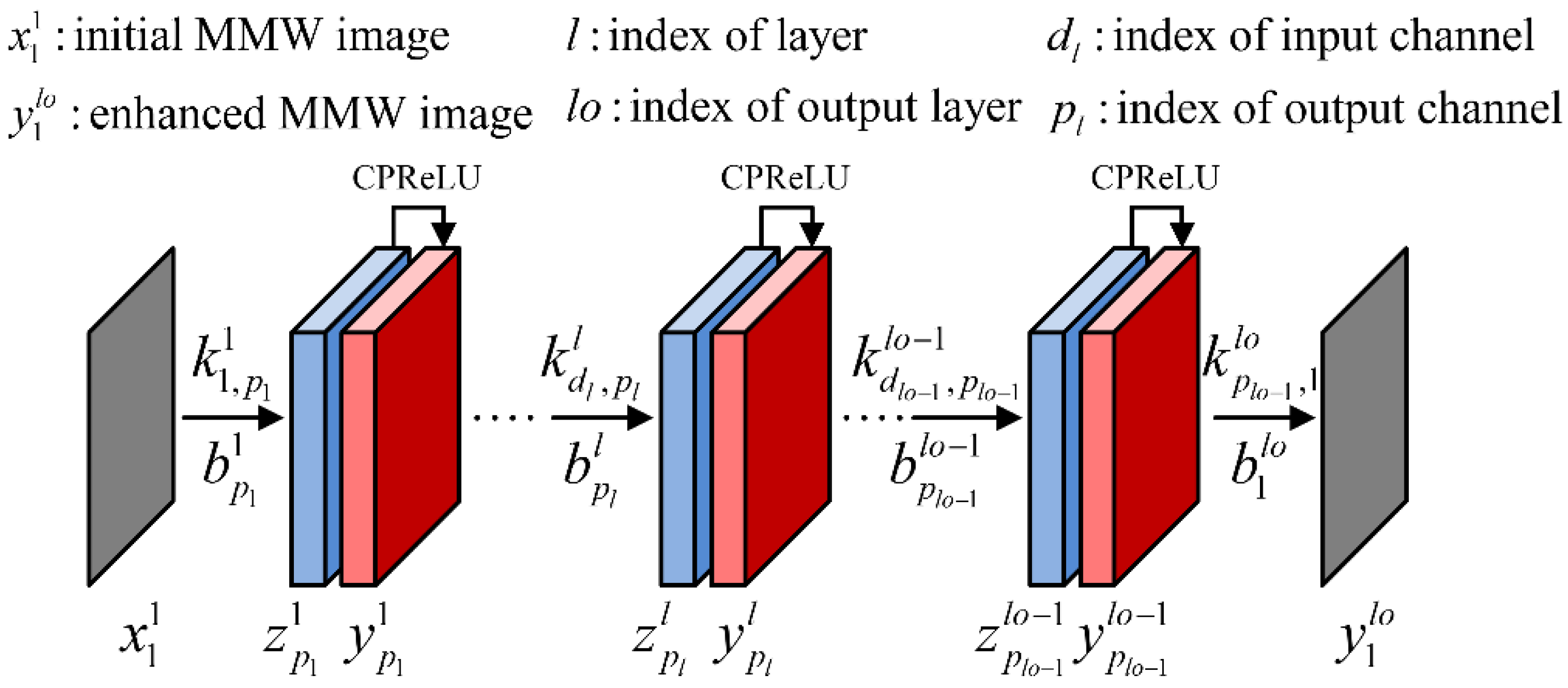
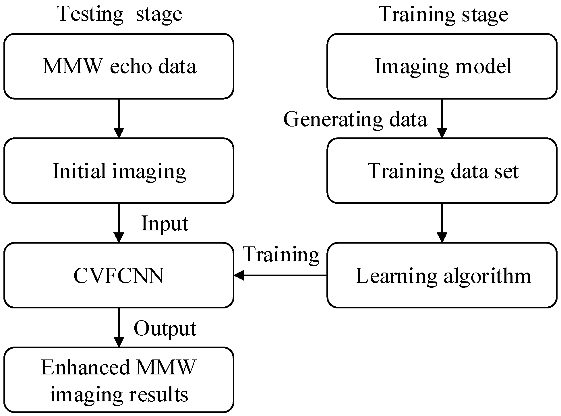
2.1. Framework of Enhanced MMW Imaging via CVFCNN

The framework of enhanced MMW 3-D imaging via a CVFCNN is shown in Figure 1. This framework is similar to the enhanced radar imaging via neural network used in [14,15,16,30,31], while the initial imaging method and the structure of a CVFCNN are different. The algorithm is divided into the training stage and the testing stage. In the training stage, the dataset is generated according to the MMW imaging model. The initial MMW images and the corresponding quality-enhanced ones are treated as the inputs and outputs of the CVFCNN model, respectively. While in the testing stage, the echo data is firstly processed with a conventional 3-D imaging algorithm to obtain the input images of the trained CVFCNN. Then, the enhanced images can be produced through the outputs of the CVFCNN.
The structure of the proposed CVFCNN is shown in Figure 2. The operations of complex convolution and multichannel summation with a bias of the convolution layer are expressed by:
z p l = d = 1 D [ Re ( k d , p l ) Re ( x d l ) Im ( k d , p l ) Im ( x d l ) ] + Re ( b p l ) + i d = 1 D [ Re ( k d , p l ) Im ( x d l ) + Im ( k d , p l ) Re ( x d l ) ] + i Im ( b p l )
where p = 1 , , P , l = 1 , , l o . For the layer, l , the numbers of input and output channels are D and P , respectively. Here, x d l C H × W represents the input feature map with a size of H × W , k d , p l C h × w denotes the convolution kernel, and b p l C is a bias. The symbol “ ” indicates a valid convolution, and z p l C H × W denotes the result of a multichannel summation with bias, where H = H h + 1 and W = W w + 1 . “Re” and “Im” indicate calculations of the real and imaginary parts of the complex variables, respectively. If we assume that the feature map size of each layer remains the same, the input x d l should be zero-padded.
Differently from the complex rectified linear unit (CReLU) used in [29,30], we present a complex parametric rectified linear unit (CPReLU) activation function, which extends the parametric rectified linear unit (PReLU) of RVNN to CVNN. A CPReLU with constant parameters, shared by real and imaginary parts, was proposed in [31]. Conversely, our proposed CPReLU has independent and learnable parameters for real and imaginary parts, respectively, which can be treated as a generalized form of CPReLU. It can adjust parameters adaptively to improve the performance of the neural network.
The output feature map y p l C H × W of layer l can be achieved by:
y p l = f ( z p l ) = max [ 0 , Re ( z p l ) ] + a R p l min [ 0 , Re ( z p l ) ] + i [ max [ 0 , Im ( z p l ) ] + a I p l min [ 0 , Im ( z p l ) ] ]
where the nonlinear activation function f ( ) is referred to as the CPReLU, and a R p l R and a I p l R are parameters of the generalized CPReLU. Then, y p l will serve as the input feature map x p l + 1 for the next layer.
The output image of the output layer l o is given by:
y 1 l o = z 1 l o
Clearly, there is no activation function in the output layer l o , thus avoiding the limitation and influence on the value range of the output image.
To further demonstrate the superiority of the proposed CPReLU, we employ the analysis method outlined in [29] to analyze the activation region of the proposed CPReLU in the complex domain, as shown in Figure 3. For the CReLU, the negative values of the real and imaginary parts are directly set to zero, so the information of these parts is lost. For CPReLU, as established in [31], since the parameter μ is a fixed value it cannot be adjusted adaptively and needs to be set manually, which is not flexible. In contrast, the parameters a R p l and a I p l for the real and imaginary parts of the proposed CPReLU are self-adaptive in the training stage of the network, so there is no need to adjust the parameters manually, which also makes the neural network more flexible in the operation of amplitude and phase.

2.2. Training Process

Given the initial image and the ground-truth image, the parameters of CVFCNN are learned end-to-end by minimizing the cost function of training data. The cost function is the sum of the squared errors (SSE), which is defined as:
E = 1 2 i = 1 H j = 1 W [ [ Re [ y 1 l o ( i , j ) ] Re [ t ( i , j ) ] ] 2 + [ Im [ y 1 l o ( i , j ) ] Im [ t ( i , j ) ] ] 2 ]
where t ( i , j ) represents the ground-truth image, and y 1 l o ( i , j ) denotes the output image. Note that this form will retain the phase of the image, which is essential for high-precision image reconstruction. The application of the image phase in target classification is also the subject of much interest [24,25,26].
The cost function in (4) is minimized by the complex-valued back propagation algorithm that calculates the derivatives of the cost function with respect to the parameters, according to the complex chain rule. The parameters are updated along the direction of negative gradient.
In the following section, we provide the formulas for calculating the gradient. Firstly, the intermediate variables, i.e., the error terms of the output layer, l o , and the hidden layer, l , are calculated, respectively, by:
δ l o = E Re ( z 1 l o ) + i E Im ( z 1 l o ) = [ Re ( y 1 l o ) Re ( t ) ] + i [ Im ( y 1 l o ) Im ( t ) ]
δ p l = E Re ( z p l ) + i E Im ( z p l ) = Re ( y p l ) Re ( z p l ) q = 1 Q [ r o t 180 ° [ Re ( k p , q l + 1 ) ] ˜ Re ( δ q l + 1 ) + r o t 180 ° [ Im ( k p , q l + 1 ) ] ˜ Im ( δ q l + 1 ) ] + i Im ( y p l ) Im ( z p l ) q = 1 Q [ - r o t 180 ° [ Im ( k p , q l + 1 ) ] ˜ Re ( δ q l + 1 ) + r o t 180 ° [ Re ( k p , q l + 1 ) ] ˜ Im ( δ q l + 1 ) ]
where “ ˜ ” is called the same convolution operation, which leads to H = H and W = W when the input and output sizes of convolution are H × W and H × W , respectively. The variable “rot180°” denotes a 180-degree rotation.
After we obtain the error terms, the derivatives of the cost function with respect to k d , p l and b p l , respectively, are given by:
E k d , p l = δ p l r o t 180 ° ( x d l ) *
E b p l = i = 1 H j = 1 W δ p l ( i , j )
where “*” denotes conjugation. The derivatives with respect to a R p l and a I p l are expressed as:
E a R p l = i = 1 H j = 1 W [ q = 1 Q [ r o t 180 ° [ Re ( k p , q l + 1 ) ] ˜ Re ( δ q l + 1 ) + r o t 180 ° [ Im ( k p , q l + 1 ) ] ˜ Im ( δ q l + 1 ) ] Re ( y p l ) a R p l ] E a I p l = i = 1 H j = 1 W [ q = 1 Q [ - r o t 180 ° [ Im ( k p , q l + 1 ) ] ˜ Re ( δ q l + 1 ) + r o t 180 ° [ Re ( k p , q l + 1 ) ] ˜ Im ( δ q l + 1 ) ] Im ( y p l ) a I p l ]
where p = 1 , , P , and P and Q denote the numbers of input and output channels for layer l + 1 , respectively.
After obtaining the derivatives of the above parameters, we employ the method of momentum stochastic gradient descent with weight decay [35] to update the parameters. In each update, the stochastic gradient descent method only selects a subset of training data to estimate the derivatives [36].

2.3. Parameter Initialization

To make the signal not be greatly amplified or weakened after passing through the multi-layer network, we need to initialize the network parameters reasonably, which contributes to ensuring the stability of the training process. For complex Gaussian random variables, when their real and imaginary parts are independent Gaussian distributions with zero mean and the same variance, their amplitude and phase obey the Rayleigh distribution and the uniform distribution, respectively [29]. For CVFCNN with CPReLU, the variance of weights is given by:
V a r ( w i l ) = 2 σ 2 = 2 / [ ( 1 + a 2 ) n l 1 ]
where i = 1 , 2 , n l 1 and the Rayleigh distribution parameter σ is:
σ = 1 / [ ( 1 + a 2 ) n l 1 ] 1 / 2
where w i l is the weight of neuron in layer l , which is chosen as k d , p l in our experiments, n l 1 is the number of neurons in the layer l 1 corresponding to w i l , and a denotes the initial value of a R p l and a I p l . Here, we choose a = 0.25 . The phase of w i l can be initialized using the uniform distribution U ( 0 , 2 π ) , and b p l can be initialized as zero.

3. Results

3.1. Numerical Simulations

The structures of several enhanced imaging approaches, based on CNN and CS, are shown in Figure 4. The phase shift migration (PSM) algorithm is used for the initial imaging, also known as the range stacking technique [37,38,39,40]. The variables CConv and Conv represent the complex and real convolutions, respectively. In the CS method, we employ the PSM operator-based CS algorithm given in [37] with the constraints of l1-norm and TV-norm. Next, we will provide comparisons of these methods through simulations and experiments.
The parameters for generating the simulated dataset are shown in Table 1. The data generation method is similar to that used in [30], but we generate the initial images using the PSM algorithm. In addition, both the initial images and the ground-truth images contain phases. For different sampling rates, 2048 groups of simulated data are generated respectively, including pairs of initial images and ground-truth images. Among them, 1920 groups of data are used as the training set, and the remaining 128 groups are treated as the testing dataset. The above neural networks are trained using the same initialization parameters. RVFCNN is initialized by the real and imaginary parts of CVFCNN. The method of momentum stochastic gradient descent with weight decay is used to update the network parameters. The momentum factor is set to be 0.5 for all parameters. For the parameters of convolution kernels and biases, the weight decay coefficient is 0.001 and the learning rate is 6 × 10⁻⁶. The parameters of CPReLU and PReLU are initialized to be 0.25 without weight decay, and the learning rate is 6 × 10⁻⁴. We trained for 8 epochs with a batch size of 16. The networks were programmed based on MATLAB, implemented on a computer platform with an Intel Xeon E5-2687W v4 CPU.
The networks are randomly initialized 5 times during training, Table 2 shows the average for the sum of the squared errors between the imaging results and the ground-truth images on the testing dataset. CPReLU1 represents the CPReLU demonstrated in [31] with constant parameters, and the parameters are set as the initial value, i.e., 0.25. CPReLU2 refers to the proposed adaptive CPReLU, with independent real and imaginary parameters. Note that the neural network methods outperform both the traditional PSM method and the CS method with respect to different data ratios. The proposed CVFCNN (CPReLU2) possesses the minimum number of errors among the neural network methods. We also note that the parameters of RVFCNN are twice those of CVFCNN [28]. Specifically, CVFCNN (CPReLU1) and CVFCNN (CPReLU2) contain 38,032 real numbers, CVFCNN (CReLU) contains 37,936 real numbers, and RVFCNN (PReLU) contains 75,968 real numbers in this example. However, RVFCNN does not perform better. The CVFCNN (CPReLU1) has relatively poor performance, which means it is unreliable to directly set a constant value as the parameter of CPReLU1. Similarly, the performance of CReLU is also inferior to that of CPReLU2, due to being without adaptive parameter adjustments.
The training time for different network architectures is shown in Table 3. We note that CVFCNN (CReLU) has the fastest training speed since the CReLU contains operations including zero. RVFCNN (PReLU) contains more channels, so the training speed is slow. The proposed CVFCNN (CPReLU2) is slightly slower than CVFCNN (CReLU) and CVFCNN (CPReLU1) because the parameters of the CPReLU2 activation function need to be updated adaptively during the training stage. However, in general, people pay more attention to the processing time of the testing stage, as shown in Table 4.
Table 4 indicates the average processing time for a single image, where GPU time means the time spent when we input the image obtained by the PSM algorithm into the neural network and evaluate the processing time on the GPU. The NVIDIA TITAN Xp card is utilized to record the GPU time. Note that the neural network methods run much faster than the CS method, due to being without iterations. In addition, in terms of CS methods, we need to readjust the parameters for different types of targets, while CNN-based methods can obtain results very rapidly after training the parameters of the network. The processing time of the proposed CVFCNN (CPReLU2) on the CPU is slightly longer than that of CVFCNN (CReLU) but with a lower SSE, as shown in Table 2. Usually, in order to obtain a better-quality image, the cost of a little processing time could be ignored. In addition, when processed by the GPU, the processing time difference between CVFCNN (CPReLU2) and CVFCNN (CReLU) in this simulation experiment is very small, being less than 0.01 s.

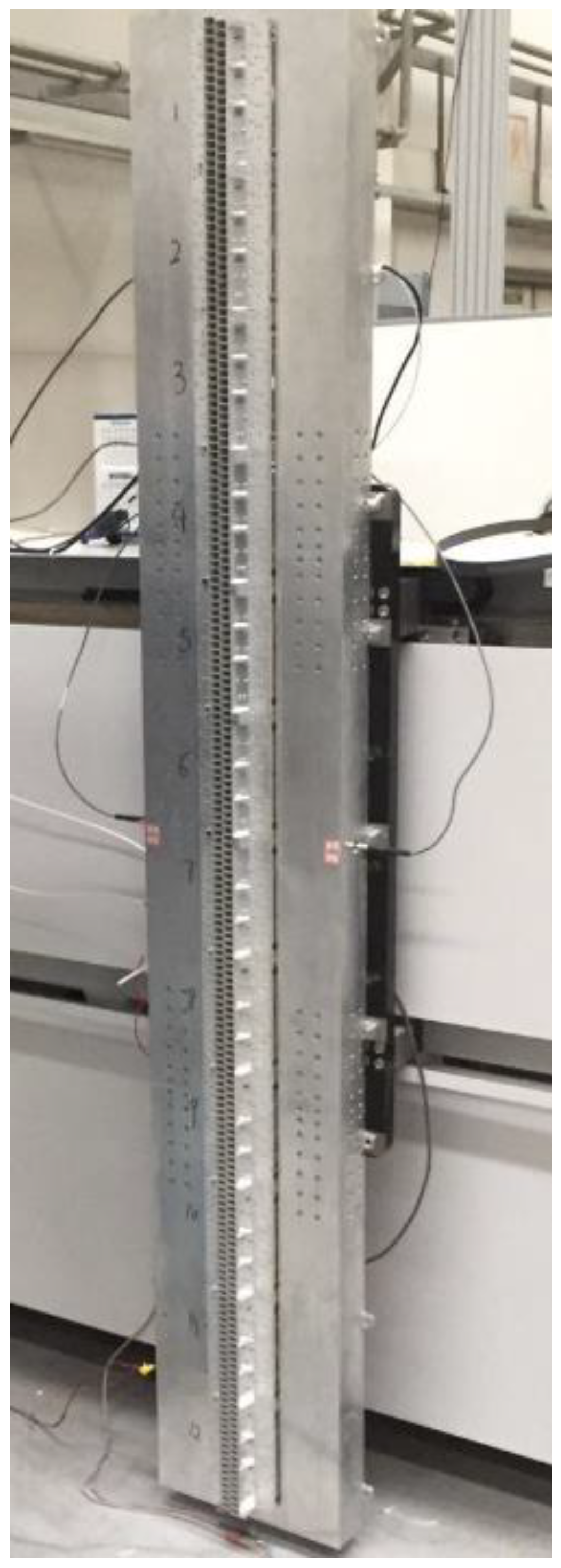
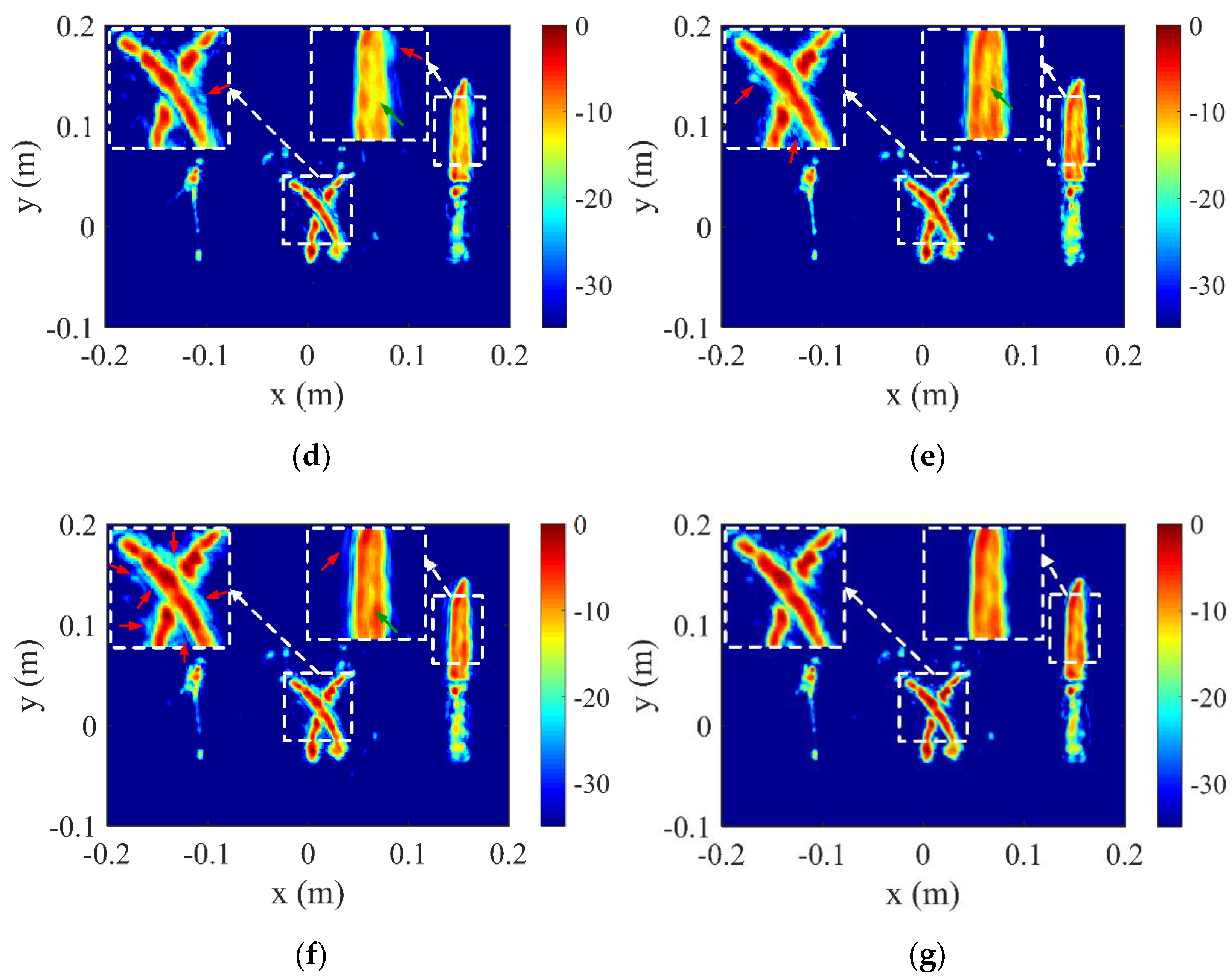
3.2. Results of the Measured Data

Here, we present experiments on the real measured data by a Ka band system operating at 32~37 GHz, as shown in Figure 5. The wide-band linear array forms a 2-D aperture through mechanical scanning. The parameters for the measured data are provided in Table 5. The measured targets are located at different distances from the antenna array, as shown in Figure 6a. The 2-D images are obtained through the maximum value projection of the 3-D results. Figure 6b demonstrates the imaging result of the PSM, using only 50% of the full data. Figure 6c illustrates the result of the CS method after repeated artificial parameter optimization. It can be seen that in order to suppress the aliasing artifacts and sidelobes of the image, the amplitudes of the targets are weakened; the parameters of the CS algorithm need to be adjusted according to the states of the scenes and the objects. Figure 6d–g shows the results of the CNN methods. Note that the CNN methods can achieve better results than the traditional PSM algorithm and perform competitively with the CS method or are even better, especially for the amplitude maintenance of the image. More importantly, CNN methods have strong robustness in terms of different objects and scenes in the testing stage. In regard to the CNN methods, as indicated by the green arrows, the amplitudes of the knife blade of CPReLU1 (Figure 6f) and CPReLU2 (Figure 6g) are more uniform than those of PReLU (Figure 6d) and CReLU (Figure 6e). Note from the detailed subfigures that the result of the proposed CPReLU2 in Figure 6g exhibits lower sidelobes than the results in Figure 6d–f, respectively, wherein the sidelobes are indicated by red arrows. The experimental results show that the proposed CPReLU2 performs best of the tested methods.
Table 6 shows the processing time of each algorithm for the measured data, which is similar to the results on the simulated testing dataset in Table 4. In the processing of measured data, the CNN-based methods are much faster than the CS method. In addition, the CNN method exhibits stronger robustness in the testing stage, and the CS method needs to readjust the algorithm parameters for different objects and scenes. The processing time of the proposed CVFCNN (CPReLU2) is slightly longer than that of CVFCNN (CReLU) but yielded better imaging results, as shown in Figure 6. Usually, in order to obtain a better-quality image, the cost of a little processing time could be ignored.

4. Conclusions

In this paper, we proposed a complex-valued fully convolutional neural network (CVFCNN) with a generalized CPReLU activation function for undersampled near-field MMW 3-D imaging. A complex-valued back-propagation algorithm was derived. Compared with the methods used in [30,31], the proposed activation function has independent parameters for the real and imaginary parts of the complex-valued data and possesses the ability of self-adaptive adjustment, which improves the performance of CVFCNN in enhanced MMW 3-D imaging. Numerical simulations and experimental results verified the effectiveness of the proposed method. The method in this paper can be applied to the fields related to radar imaging. Compared with the classical ReLU-based activation function, the proposed CPReLU activation function preserves phase information that is useful for radar signal processing. Future work will apply the proposed method to more valuable research and application scenarios.

Author Contributions

Conceptualization, H.J. and S.L.; methodology, H.J., S.L., K.M. and S.W.; software, H.J.; validation, H.J., S.L. and X.C.; formal analysis, H.J. and S.L.; investigation, H.J., S.L., K.M., S.W. and X.C.; resources, S.L., X.C., G.Z. and H.S.; data curation, H.J. and X.C.; writing—original draft preparation, H.J.; writing—review and editing, S.L.; visualization, H.J.; supervision, S.L., G.Z. and H.S.; project administration, S.L., G.Z. and H.S.; funding acquisition, S.L., G.Z. and H.S. All authors have read and agreed to the published version of the manuscript.

Funding

This research was supported by the National Natural Science Foundation of China under Grant 61771049.

Conflicts of Interest

The authors declare no conflict of interest.

References

  1. Casalini, E.; Frioud, M.; Small, D.; Henke, D. Refocusing FMCW SAR Moving Target Data in the Wavenumber Domain. IEEE Trans. Geosci. Remote Sens. 2019, 57, 3436–3449. [Google Scholar] [CrossRef]
  2. Wang, H.; Zhang, H.; Dai, S.; Sun, Z. Azimuth Multichannel GMTI Based on Ka-Band DBF-SCORE SAR System. IEEE Geosci. Remote Sens. Lett. 2018, 15, 419–423. [Google Scholar] [CrossRef]
  3. Amin, M. Radar for Indoor Monitoring: Detection, Classification, and Assessment; CRC Press: Boca Raton, FL, USA, 2017. [Google Scholar]
  4. Sheen, D.; McMakin, D.; Hall, T. Near-Field Three-Dimensional Radar Imaging Techniques and Applications. Appl. Opt. 2010, 49, 83–93. [Google Scholar] [CrossRef] [PubMed]
  5. Sheen, D.M.; McMakin, D.L.; Hall, T.E. Three-Dimensional Millimeter-Wave Imaging for Concealed Weapon Detection. IEEE Trans. Microw. Theory Tech. 2001, 49, 1581–1592. [Google Scholar] [CrossRef]
  6. Oliveri, G.; Salucci, M.; Anselmi, N.; Massa, A. Compressive Sensing as Applied to Inverse Problems for Imaging: Theory, Applications, Current Trends, and Open Challenges. IEEE Antennas Propag. Mag. 2017, 59, 34–46. [Google Scholar] [CrossRef]
  7. Rani, M.; Dhok, S.B.; Deshmukh, R.B. A Systematic Review of Compressive Sensing: Concepts, Implementations and Applications. IEEE Access 2018, 6, 4875–4894. [Google Scholar] [CrossRef]
  8. Upadhyaya, V.; Salim, D.M. Compressive Sensing: Methods, Techniques, and Applications. IOP Conf. Ser. Mater. Sci. Eng. 2021, 1099, 012012. [Google Scholar] [CrossRef]
  9. Seyfioglu, M.S.; Erol, B.; Gurbuz, S.Z.; Amin, M.G. DNN Transfer Learning from Diversified Micro-Doppler for Motion Classification. IEEE Trans. Aerosp. Electron. Syst. 2019, 55, 2164–2180. [Google Scholar] [CrossRef] [Green Version]
  10. Erol, B.; Gurbuz, S.Z.; Amin, M.G. Motion Classification Using Kinematically Sifted ACGAN-Synthesized Radar Micro-Doppler Signatures. IEEE Trans. Aerosp. Electron. Syst. 2020, 56, 3197–3213. [Google Scholar] [CrossRef] [Green Version]
  11. Skaria, S.; Al-Hourani, A.; Lech, M.; Evans, R.J. Hand-Gesture Recognition Using Two-Antenna Doppler Radar with Deep Convolutional Neural Networks. IEEE Sens. J. 2019, 19, 3041–3048. [Google Scholar] [CrossRef]
  12. Chen, Z.; Li, G.; Fioranelli, F.; Griffiths, H. Dynamic Hand Gesture Classification Based on Multistatic Radar Micro-Doppler Signatures Using Convolutional Neural Network. In Proceedings of the 2019 IEEE Radar Conference (RadarConf), Boston, MA, USA, 22–26 April 2019; pp. 1–5. [Google Scholar]
  13. Qin, D.; Liu, D.; Gao, X.; Jingkun, G. ISAR Resolution Enhancement Using Residual Network. In Proceedings of the 2019 IEEE 4th International Conference on Signal and Image Processing (ICSIP), Wuxi, China, 19–21 July 2019; pp. 788–792. [Google Scholar]
  14. Gao, X.; Qin, D.; Gao, J. Resolution Enhancement for Inverse Synthetic Aperture Radar Images Using a Deep Residual Network. Microw. Opt. Technol. Lett. 2020, 62, 1588–1593. [Google Scholar] [CrossRef]
  15. Hu, C.; Wang, L.; Li, Z.; Zhu, D. Inverse Synthetic Aperture Radar Imaging Using a Fully Convolutional Neural Network. IEEE Geosci. Remote Sens. Lett. 2020, 17, 1203–1207. [Google Scholar] [CrossRef]
  16. Yang, T.; Shi, H.; Lang, M.; Guo, J. ISAR Imaging Enhancement: Exploiting Deep Convolutional Neural Network for Signal Reconstruction. Int. J. Remote Sens. 2020, 41, 9447–9468. [Google Scholar] [CrossRef]
  17. Cheng, Q.; Ihalage, A.A.; Liu, Y.; Hao, Y. Compressive Sensing Radar Imaging With Convolutional Neural Networks. IEEE Access 2020, 8, 212917–212926. [Google Scholar] [CrossRef]
  18. Mu, H.; Zhang, Y.; Ding, C.; Jiang, Y.; Er, M.H.; Kot, A.C. DeepImaging: A Ground Moving Target Imaging Based on CNN for SAR-GMTI System. IEEE Geosci. Remote Sens. Lett. 2021, 18, 117–121. [Google Scholar] [CrossRef]
  19. Pu, W. Shuffle GAN with Autoencoder: A Deep Learning Approach to Separate Moving and Stationary Targets in SAR Imagery. IEEE Trans. Neural Netw. Learn. Syst. 2021, 1–15. [Google Scholar] [CrossRef] [PubMed]
  20. Ding, J.; Wen, L.; Zhong, C.; Loffeld, O. Video SAR Moving Target Indication Using Deep Neural Network. IEEE Trans. Geosci. Remote Sens. 2020, 58, 7194–7204. [Google Scholar] [CrossRef]
  21. Fang, S.; Nirjon, S. SuperRF: Enhanced 3D RF Representation Using Stationary Low-Cost MmWave Radar. In Proceedings of the International Conference on Embedded Wireless Systems and Networks (EWSN), Lyon, France, 17–19 February 2020; Volume 2020, pp. 120–131. [Google Scholar]
  22. Sun, Y.; Huang, Z.; Zhang, H.; Cao, Z.; Xu, D. 3DRIMR: 3D Reconstruction and Imaging via MmWave Radar Based on Deep Learning. arXiv 2021, arXiv:2108.02858. [Google Scholar]
  23. Guan, J.; Madani, S.; Jog, S.; Gupta, S.; Hassanieh, H. Through Fog High-Resolution Imaging Using Millimeter Wave Radar. In Proceedings of the IEEE/CVF Conference on Computer Vision and Pattern Recognition (CVPR), Seattle, WA, USA, 13–19 June 2020. [Google Scholar]
  24. Gao, J.; Qin, Y.; Deng, B.; Wang, H.; Li, X. A Novel Method for 3-D Millimeter-Wave Holographic Reconstruction Based on Frequency Interferometry Techniques. IEEE Trans. Microw. Theory Tech. 2018, 66, 1579–1596. [Google Scholar] [CrossRef]
  25. Minin, I.V.; Minin, O.V.; Castineira-Ibanez, S.; Rubio, C.; Candelas, P. Phase Method for Visualization of Hidden Dielectric Objects in the Millimeter Waveband. Sensors 2019, 19, 3919. [Google Scholar] [CrossRef] [PubMed] [Green Version]
  26. Sadeghi, M.; Tajdini, M.M.; Wig, E.; Rappaport, C.M. Single-Frequency Fast Dielectric Characterization of Concealed Body-Worn Explosive Threats. IEEE Trans. Antennas Propag. 2020, 68, 7541–7548. [Google Scholar] [CrossRef]
  27. Aizenberg, N.N.; Ivaskiv, Y.L.; Pospelov, D.A.; Hudiakov, G.F. Multivalued Threshold Functions in Boolean Complex-Threshold Functions and Their Generalization. Cybern. Syst. Anal. 1971, 7, 626–635. [Google Scholar] [CrossRef]
  28. Hirose, A. Complex-Valued Neural Networks: Advances and Applications; Wiley: New York, NY, USA, 2013. [Google Scholar]
  29. Trabelsi, C.; Bilaniuk, O.; Zhang, Y.; Serdyuk, D.; Subramanian, D.; Santos, J.F.; Mehri, S.; Rostamzadeh, N.; Bengio, Y.; Pal, C.J. Deep Complex Networks. In Proceedings of the ICLR 2018 Conference, Vancouver, BC, Canada, 30 April–3 May 2018. [Google Scholar]
  30. Gao, J.; Deng, B.; Qin, Y.; Wang, H.; Li, X. Enhanced Radar Imaging Using a Complex-Valued Convolutional Neural Network. IEEE Geosci. Remote Sens. Lett. 2019, 16, 35–39. [Google Scholar] [CrossRef] [Green Version]
  31. Zhang, Y.; Yang, Q.; Zeng, Y.; Deng, B.; Wang, H.; Qin, Y. High-Quality Interferometric Inverse Synthetic Aperture Radar Imaging Using Deep Convolutional Networks. Microw. Opt. Technol. Lett. 2020, 62, 3060–3065. [Google Scholar] [CrossRef]
  32. Pu, W. Deep SAR Imaging and Motion Compensation. IEEE Trans. Image Process. 2021, 30, 2232–2247. [Google Scholar] [CrossRef] [PubMed]
  33. Mu, H.; Zhang, Y.; Jiang, Y.; Ding, C. CV-GMTINet: GMTI Using a Deep Complex-Valued Convolutional Neural Network for Multichannel SAR-GMTI System. IEEE Trans. Geosci. Remote Sens. 2022, 60, 5201115. [Google Scholar] [CrossRef]
  34. Shelhamer, E.; Long, J.; Darrell, T. Fully Convolutional Networks for Semantic Segmentation. IEEE Trans. Pattern Anal. Mach. Intell. 2017, 39, 640–651. [Google Scholar] [CrossRef]
  35. Sutskever, I.; Martens, J.; Dahl, G.; Hinton, G. On the Importance of Initialization and Momentum in Deep Learning. In Proceedings of the 30th International Conference on International Conference on Machine Learning, Atlanta, GA, USA, 16–21 June 2013. [Google Scholar]
  36. Bengio, Y. Practical recommendations for gradient-based training of deep architectures. In Neural Networks: Tricks of the Trade; Springer: Berlin/Heidelberg, Germany, 2012; pp. 437–478. [Google Scholar]
  37. Li, S.; Zhao, G.; Sun, H.; Amin, M. Compressive Sensing Imaging of 3-D Object by a Holographic Algorithm. IEEE Trans. Antennas Propag. 2018, 66, 7295–7304. [Google Scholar] [CrossRef]
  38. Yang, G.; Li, C.; Wu, S.; Liu, X.; Fang, G. MIMO-SAR 3-D Imaging Based on Range Wavenumber Decomposing. IEEE Sens. J. 2021, 21, 24309–24317. [Google Scholar] [CrossRef]
  39. Gao, H.; Li, C.; Zheng, S.; Wu, S.; Fang, G. Implementation of the Phase Shift Migration in MIMO-Sidelooking Imaging at Terahertz Band. IEEE Sens. J. 2019, 19, 9384–9393. [Google Scholar] [CrossRef]
  40. Tan, W.; Huang, P.; Huang, Z.; Qi, Y.; Wang, W. Three-Dimensional Microwave Imaging for Concealed Weapon Detection Using Range Stacking Technique. Int. J. Antennas Propag. 2017, 2017, 1480623. [Google Scholar] [CrossRef] [Green Version]
Figure 1. Framework of enhanced MMW 3-D imaging via the CVFCNN.
Electronics 11 00147 g001
Figure 2. Framework of the CVFCNN with a CPReLU activation function.
Electronics 11 00147 g002
Figure 3. Active regions of different activation functions: (a) CReLU; (b) CPReLU [31]; (c) proposed CPReLU.
Electronics 11 00147 g003
Figure 4. Structures of enhanced MMW 3-D imaging: (a) the proposed CVFCNN (CPReLU); (b) RVFCNN (PReLU); (c) CVFCNN (CReLU); (d) operator-based CS.
Electronics 11 00147 g004
Figure 5. Imaging system.
Electronics 11 00147 g005
Figure 6. Images showing the 2-D images using 50% of data: (a) the measured targets; (b) image via PSM; (c) image via CS; (d) image via RVFCNN (PReLU); (e) image via CVFCNN (CReLU); (f) image via CVFCNN (CPReLU1); (g) image via CVFCNN (CPReLU2).
Electronics 11 00147 g006aElectronics 11 00147 g006b
Table 1. Parameters for generating simulated data.
ParameterValue
Frequency (GHz)34.5
Aperture size (m)0.25 × 0.25
Sampling interval (mm)5
Imaging range (m)0.25 m~0.45 m
Beam width of antenna element (°)55
Original resolution (mm)5
Enhanced imaging resolution (mm)2.5
Image pixels256 × 256
Table 2. Average SSE between imaging results and ground-truth images on the testing dataset.
Methods25% Data50% Data75% Data100% Data
PSM1214.51653.47392.01261.44
PSM-CS142.3762.6556.9355.84
RVFCNN (PReLU)83.5758.5447.8239.68
CVFCNN (CReLU)83.8259.1448.0239.93
CVFCNN (CPReLU1)84.8761.3950.4742.67
CVFCNN (CPReLU2)82.7458.2147.1839.19
Table 3. Training-time comparison on the training dataset.
MethodsCPU(h)
RVFCNN (PReLU)22.6
CVFCNN (CReLU)13.3
CVFCNN (CPReLU1)15.2
CVFCNN (CPReLU2)15.4
Table 4. Processing-time comparison on the testing dataset.
MethodsCPU(s)GPU(s)
PSM0.12/
PSM-CS22.82/
RVFCNN (PReLU)1.180.10
CVFCNN (CReLU)0.710.08
CVFCNN (CPReLU1)0.720.08
CVFCNN (CPReLU2)0.720.08
Table 5. Parameters for Measured Data.
ParameterValue
Center frequency (GHz)34.5
Bandwidth (GHz)5
Sampling interval (mm)Δx = 4, Δy = 5
Beam width of antenna element (°)55
Imaging range (m)0.3 m~0.42 m
Imaging range interval (mm)5
Imaging range slices25
Image pixels768 × 768
Table 6. Processing-time comparison of measured data.
MethodsCPU(s)GPU(s)
PSM4.5/
PSM-CS647.2/
RVFCNN (PReLU)240.216.4
CVFCNN (CReLU)143.611.9
CVFCNN (CPReLU1)145.312.2
CVFCNN (CPReLU2)145.312.2
Publisher’s Note: MDPI stays neutral with regard to jurisdictional claims in published maps and institutional affiliations.

