Assessment of Various Window Functions in Spectral Identification of Passive Intermodulation

Abstract

Passive Intermodulation (PIM) distortion is a major problem in wireless communications which limits cell coverage and data rates. Passive nonlinearities result in weak intermodulation (IMD) products that are very difficult to diagnose, troubleshoot and model. To predict PIM, behavioral models are used where spectral components of PIM are estimated from the power spectral density at the output of the model. The primary goal of this paper is to study the effect of window functions on the capability of the power spectral density computed from the periodogram of signal realizations to predict low power PIM components in a wideband multichannel communication system. Different window functions are analyzed and it is shown that windows with high side-lobe level fail to predict PIM components which are close to the main channels due to their high spectral leakage; while window functions with low roll-off rate of the side lobes fail to predict low power higher order PIM components especially when the frequency separation between the main carriers is high. These results are supported by simulations of the power spectral density computed using signal realizations of an LTE carrier aggregated system.

1. Introduction

Passive intermodulation (PIM) distortion has been a significant problem in modern mobile communication systems as it limits system performance and capacity. Unlike active nonlinear distortion which is usually manifested as intermodulation (IMD) products with significant power levels, passive nonlinearities result in very weak IMD products which make it very difficult to measure and model [1]. In carrier aggregated systems such as 4G systems, PIM is manifested as IMD components which result in interference with the main channels in the receive band.

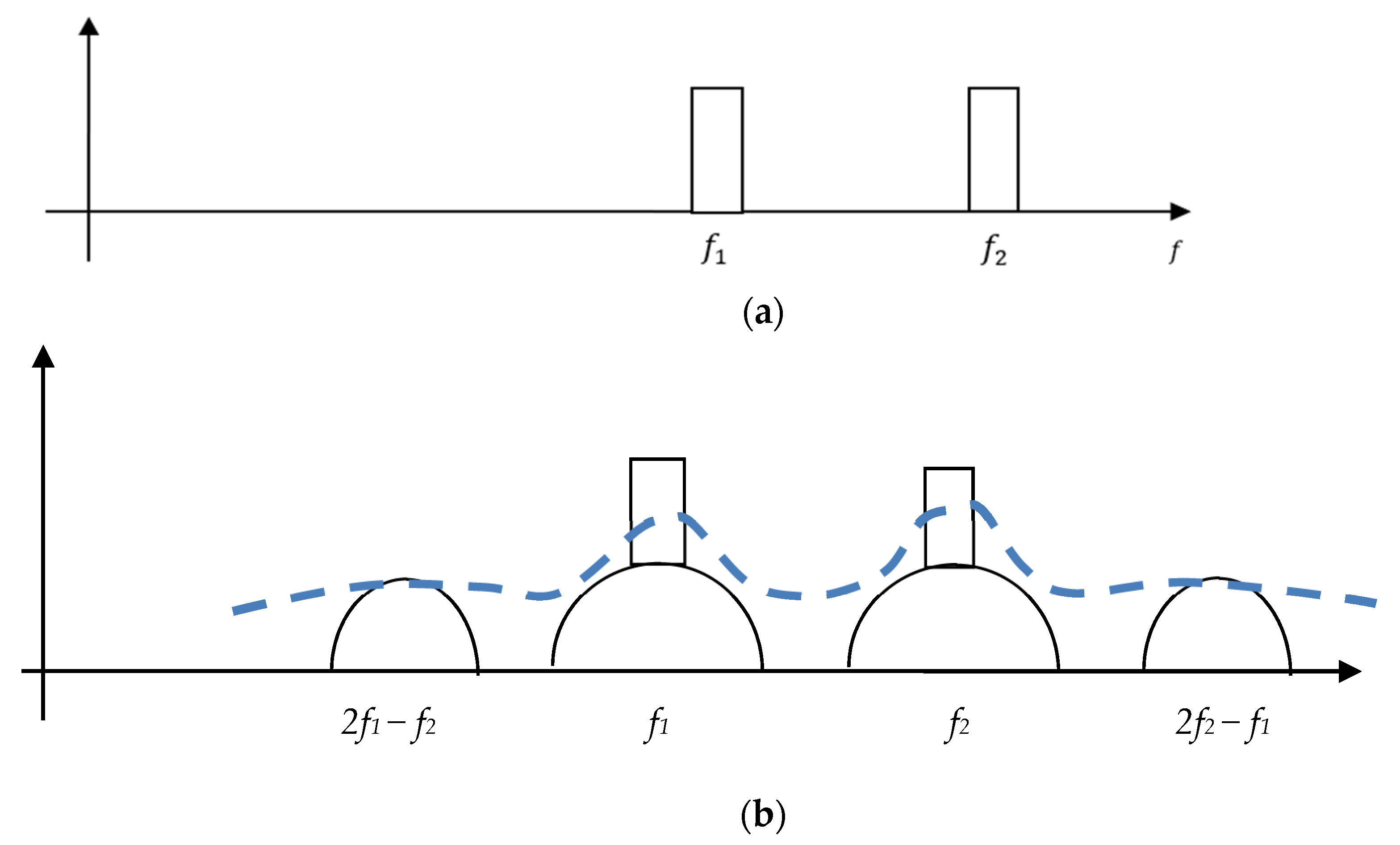
A simple illustration of PIM in wireless systems is shown in Figure 1a where the input to the passive nonlinearity consists of two band pass signals centered at frequencies $f_1$ and $f_2$. The power spectral density (PSD) of the output of the nonlinearity is shown in Figure 1b which consists of the spectra at the fundamental frequencies in addition to the IMD components at frequencies $2f_1-f_2$ and $2f_2-f_1$ which may lie within the receive band 2. In this scenario, the IMD components produced by the passive nonlinearity can result in significant interference in the receive band which limits system performance and capacity.

To predict PIM in in such scenarios, behavioral models that relate the output PIM to the input signal level and frequency are used [2,3,4,5,6,7,8,9,10]. Behavioral models are developed using measured characteristics of the nonlinear device and then they can be used to predict PIM from the computation of the power spectrum at the output of the model.

Estimating PIM from the power spectral density at the output of the behavioral model using direct application of the Fast Fourier Transform (FFT) to a signal realization can be a simple task when the power level of the IMD components is high as the case of active nonlinearities (above −60 dBc). 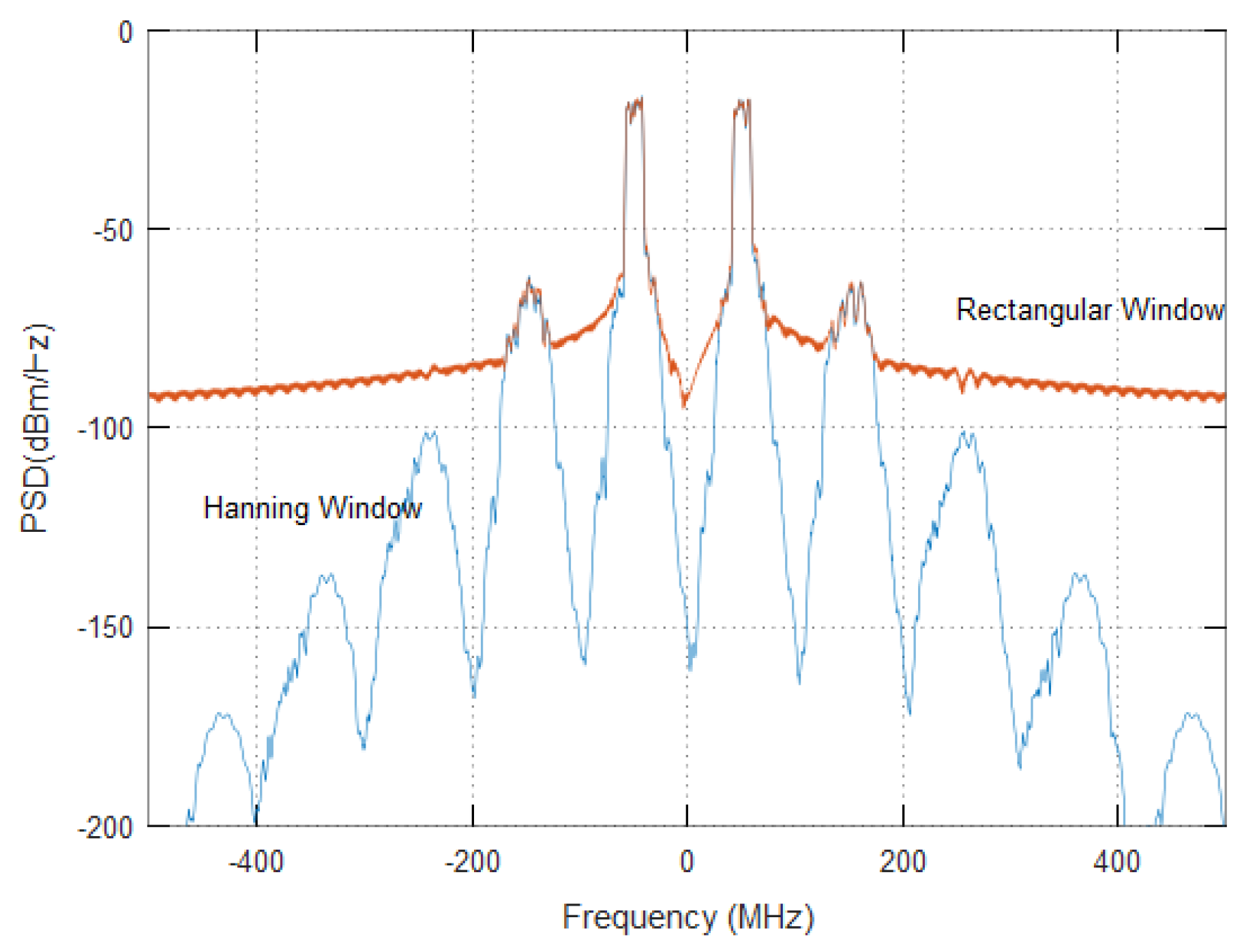However, with passive nonlinearity, the IMD components can have power levels of less than −140 dBc which makes it difficult to predict PIM [7,8]. The reason for this is that the finite length of signal realizations results in high levels of spectral leakage in the computed power spectrum which tends to obscure the IMD components as spectral leakage level are usually much higher than the intermodulation power level.

Figure 1b shows an illustration of this phenomenon where spectral leakage that results from the Fast Fourier Transform (FFT) makes it impossible to predict IMD components from weak passive nonlinearities. In principle, the frequency of intermodulation spectra and their power level depend on the frequency separation between the main channels and the input power and, thus, it is important to use an appropriate spectral estimation algorithm so that these IMD components can be predicted.

Spectral leakage can be minimized through windowing where signal samples are weighted by a given time window which enhances the accuracy of spectral estimation [11]. The type of the window has a significant impact on spectral leakage where low-peak side lobe of the frequency response of the window function indicates small spectral leakage. Several window functions have been used in the literature for suppression of spectral leakage [12,13,14]. However, the choice of the window function is a compromise between the amount of spectral leakage and the frequency resolution and, hence, the computational complexity of computing the windowed FFT [3].

This problem has been studied in the context of prediction and reduction of harmonics in power systems where it was shown that the direct application of the FFT has inherent performance limitations, such as spectral leakage and the picket fence effect [11]. However, limed research has been done on the effect of selection of window functions on spectral identification of PIM. This paper aims to provide an assessment of the performance of various window functions on in the ability of the power spectral density to predict the IMD components in a wideband system. The significance of this research in that the results presented can be used in the design of simulation models and measurements setups for accurate prediction or measurement of PIM in wireless systems.

This paper provides an analysis of passive nonlinearity in a carrier aggregated system using a polynomial based behavioral model and develops the output of the nonlinearity for two carrier aggregated signals which represents the practical scenario by which PIM is manifested in wireless system. Next, the paper provides a theoretical study of power spectral density of the output of the passive nonlinearity where the characteristics of various window functions which are used to overcome spectral leakage are explored. The last section provides simulation results which quantify the ability of power spectrum computed using various window functions to predict passive intermodulation levels.

2. Modeling of Passive Intermodulation

Perhaps, the most common approach to modeling nonlinearity is the Volterra like approaches [15]. One of the most common simplifications of Volterra models is the memoryless polynomial model which has extensively been used to model active nonlinearities with no memory effects. The response of an RF nonlinearity to multiple signals in a carrier aggregation system such as LTE system was studied in [16], where the response of a memoryless polynomial model to multiple communication signals at multiple carrier frequencies of the form.

$$x\left(t\right)={{\displaystyle \sum }}_{m=-K}^M\frac{1}{2}{x}_m\left(t\right)e^{j2\pi f_{m}t}$$

(1)

where $x_m\left(t\right)$ is the complex envelope of the input signals centered at frequencies $f_m \mathrm{and} K \mathrm{indicates}\mathrm{the}\mathrm{number}\mathrm{of}\mathrm{signals}$. The analysis in [17] was based on multinomial analysis of the polynomial model which can be described as:

$$y\left(t\right)={{\displaystyle \sum }}_{n=1}^N{y}_n\left(t\right)$$

(2)

where $y_n\left(t\right)=a_n{x}^n\left(t\right)$, an represents the n-th order coefficient of the memoryless nonlinearity and N is the nonlinear order. Note that only odd order polynomial terms are considered in this model as the passive nonlinearity is considered to have an odd symmetry in its I/V characteristic [17]. This means that the model can only model IMD components that lie within the proximity of the carrier in the frequency spectrum, which is a reasonable assumption as low frequency IMD components that result from even IMD products can usually be removed by filtering.

To analyze the response of the nonlinearity to multiple signals, the output of the nonlinearity can be found by inserting (1) into (2) where the n-th order nonlinearity can be written as:

$$y_n\left(t\right)=\left(\frac{a_n}{2^n}\right){\left(x_m\left(t\right)e^{j2\pi f_{m}t}\right)}^n={\displaystyle \sum }_{n_{-M}{f}_{-M}+\dots +n_M{f}_M=f}\frac{a_n}{2^n}\left(\begin{array}{c}n\\ n_{-M}\dots .,n_M\end{array}\right)\left({\displaystyle \prod }_{i=1}^n{x}_{m_i}{e}^{j2\pi ft}+x_{m_i}^{*}{e}^{-j2\pi ft}\right)$$

(3)

The case of two signals at frequencies f₁ and f₂ is unique as it makes the analysis more tractable and; at the same time, this enables nonlinear distortion to be quantified and predicted at IMD frequencies in a wideband carrier aggregated wireless system. For a two-signal input, the passive nonlinearity results in IMD components at the IMD frequencies. In this scenario, the input to the passive nonlinearity is represented as

$$x\left(t\right)=A_1\left(t\right)\cos \left(2\pi f_{1}t+{\varphi }_1\left(t\right)\right)+A_2\left(t\right)\cos \left(2\pi f_{2}t+{\varphi }_2\left(t\right)\right)$$

(4)

The complex envelop of the input signal can be written as

$$\tilde{x}\left(t\right)=A_1\left(t\right)e^{{\varphi }_1\left(t\right)}{e}^{-2\pi f_{0}t}+A_2\left(t\right)e^{{\varphi }_2\left(t\right)}{e}^{2\pi f_{0}t}$$

(5)

where $f_0=\frac{f_2-f_1}{2}$.

As shown in [17], by inserting (5) into (3), the output of the nonlinearity in (2) consists of the fundamental signals at frequencies $-f_0$ and $f_0$ in addition to the IMD components at the IMD frequencies as shown in

Table 1. IMD frequencies for a two-tone input.

N	Upper Intermod (Band Pass)	Upper Intermod (Envelop)	Lower Intermod (Band Pass)	Lower Intermod (Envelop)
3	$2f_2-f_1$	$3f_0$	$2f_1-f_2$	$-3f_0$
5	$3f_2-2f_1$	$5f_0$	$3f_1-2f_2$	$-5f_0$
7	$4f_2-3{\omega }_1$	$7f_0$	$4f_1-3f_2$	$-7f_0$
9	$5f_2-4f_1$	$9f_0$	$5f_1-4f_2$	$-9f_0$
11	$6f_2-5f_1$	$11f_0$	$6f_2-5f_1$	$-11f_0$

below. The output of the polynomial model at the fundamental frequencies can be as [17]:

$${\tilde{z}}_{f_0}\left(t\right)={\displaystyle \sum }_{n=1}^N{\displaystyle \sum }_{l=0}^{\frac{n-1}{2}}{b}_{n,l}{\tilde{u}}_{-2}^l{\tilde{u}}_{-1}^{\frac{n-1}{2}-l} {\tilde{u}}_1^{\frac{n+1}{2}-l}{\tilde{u}}_2^l$$

(6)

where

$$b_{n,l}=a_n{2}^{n-1}\left(\begin{array}{c}n\\ l,\frac{n-1}{2}-l,\frac{n+1}{2}+l, l\end{array}\right)$$

This expression represents the output of nonlinearity at the first carrier and captures nonlinear distortion that results from the interaction of the two signals by nonlinearity. In a similar manner, the third order IMD components at the lower IMD frequency 3f₀ can be found as [17]

$${\tilde{z}}_{3f_0}\left(t\right)={\displaystyle \sum }_{n=1}^N{\displaystyle \sum }_{l=0}^{\frac{n-2}{2}}{b}_{n,l}{\tilde{u}}_{-2}^{l+1}{\tilde{u}}_{-1}^{\frac{n-3}{2}-l} {\tilde{u}}_1^{\frac{n+1}{2}-l}{\tilde{u}}_2^l$$

(7)

where

$$b_{n,l}=\frac{a_n}{2^{n-1}}\left(\begin{array}{c}n\\ \frac{n-3}{2}-l,l+1,l,\frac{n+1}{2}-l\end{array}\right)$$

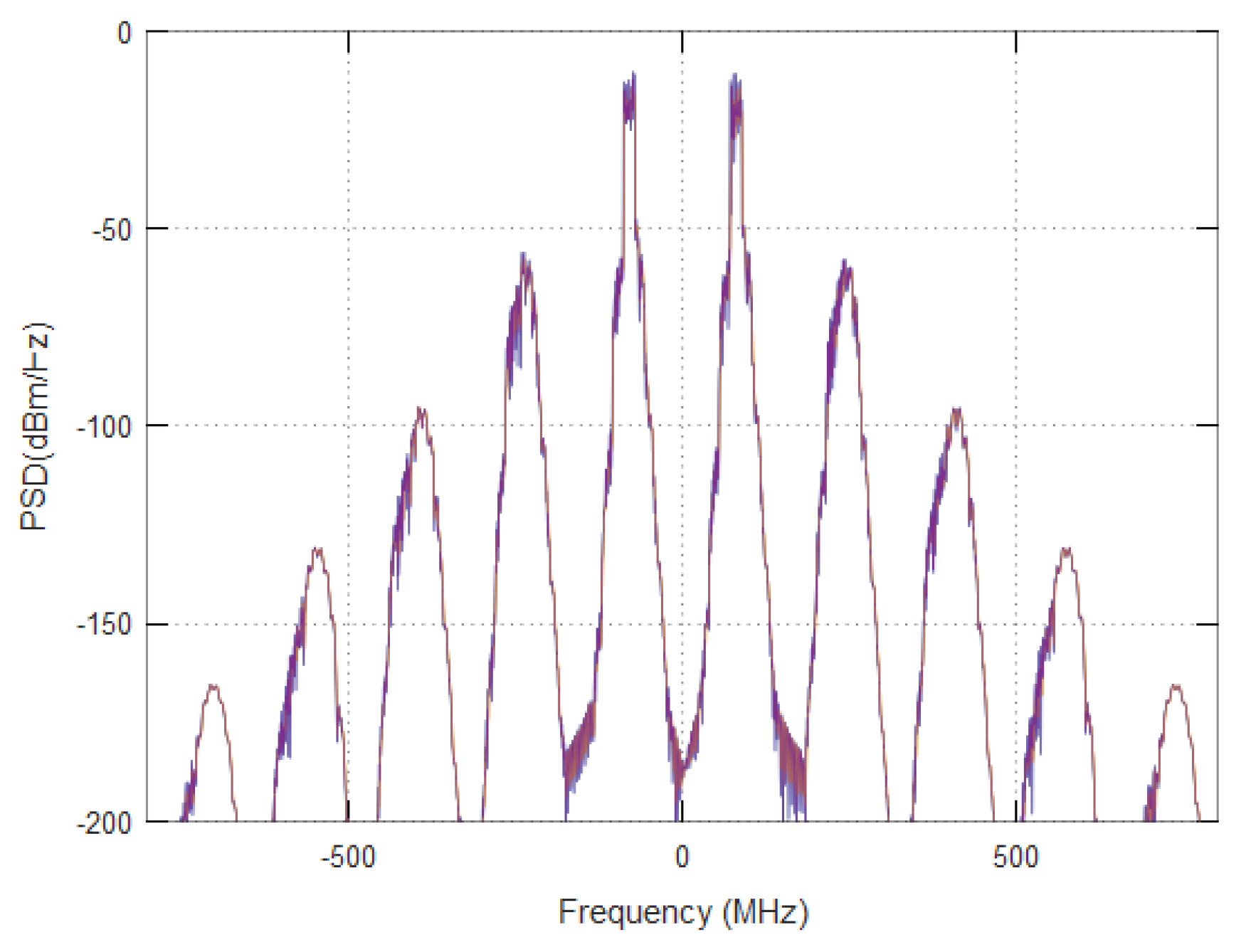
and higher order IMD components can be derived in a similar way. The above analysis enables PIM in carrier aggregation systems to be predicted. In the above formulation, PIM is manifested as gain compression, spectral regrowth and cross modulation distortions at the carrier frequency plus a nonlinear distortion component with a wider bandwidth at the intermodulation frequency. Figure 2 shows the output spectra of a passive nonlinearity to the sum of two OFDM signals each of which has a 20 MHz bandwidth with a frequency separation of 120 MHz between them. The figure shows the IMD components which appear at 360, 600, 840, 1080 MHz respectively. Note that the widened spectrum at the fundamental frequency −f₀ represents the spectral regrowth and cross modulation while the spectral components at the IMD frequencies which may interfere with other channels in a carrier aggregation system or with the receive bands.

3. Estimation of Power Spectral Density of the Output of a Passive Nonlinearity

The power spectral density of a random signal is defined as the statistical average of the signal periodogram of signal realizations of infinite lengths [11]:

$$S_{xx}\left(\omega \right)=E\{\underset{M\to \infty }{lim}{p}_{x,M}\left(\omega \right)\}$$

(8)

where

$$\begin{array}{c}{p}_{x,M}\left(\omega \right)=\frac{1}{M}|DTFT(x\left(n\right){|}^2|=\frac{1}{M}{\left|{\displaystyle {\displaystyle \sum }_{n=0}^{M-1}}x\left(n\right)e^{-j\omega n}\right|}^2\\ \iff \frac{1}{M}{\displaystyle {\displaystyle \sum }_{n=0}^{M-1-\left|l\right|}}x\left(n\right)x\left(n+\left|l\right|\right)\end{array}$$

(9)

is the periodogram of the output signal which is basically the squared magnitude of the DTFT of the signal realization of a finite length M. Therefore, the periodogram represents an unbiased estimate of the power spectral density (PSD) which is a random variable with zero mean, but has a non-zero variance as it represents a single realization of the signal [11]. Note that the periodogram of finite length signal does not represent the PSD of the signal as the PSD in (8) assumes a signal of infinite length; however, the accuracy of the periodogram in representing the PSD increases as the length of the signal realization used is increased. The finite length of the signal realization results in spectral leakage where extra frequency components are generated in the vicinity of the main frequency component [13]. Spectral leakage results in the inability of the periodogram to represent other frequency components of the signal such as harmonics and IMD components.

To overcome the problem of spectral leakage, the input signal is multiplied by a window function where any finite length signal is viewed as having an infinite length when viewed from a window of a finite length and, hence, the periodogram can better represent the actual PSD from a finite length realization of the signal as will be seen in the following section. The periodogram of the windowed signal is called the modified periodogram and is expressed as [11]:

$$p_{x_w,M}\left(\omega \right)=\frac{1}{M}\left|DTFT(x_w\left(n\right){|}^2\right|=\frac{1}{M}{\left|{\displaystyle \sum }_{n=0}^{M-1}{x}_w\left(n\right)e^{-j\omega n}\right|}^2$$

(10)

where $x_w\left(n\right)=x\left(n\right)w\left(n\right)$ is the windowed signal and $w\left(t\right)$ is the window function and M is the signal size. The windowed periodogram can enhance the accuracy of the spectral analysis of the PIM components and produce better estimates of nonlinear distortion.

Note that the periodogram is an estimate of the PSD of the signal. The accuracy of the estimate depends on the bias of the estimate while its precision depends on the mean squared error. The bias of the estimate results in spectral leakage while the variance of the estimate results in inconsistency of the estimate. The periodogram of a finite length signal is always a biased estimate of the PSD but this the bias can be controlled by windowing. A larger window size (Ts) which means higher resolution (1/Ts) results in smoother transitions which means less bias of the estimate and hence, less spectral leakage. Therefore, the choice of the window function depends on a compromise between the amount of spectral leakage and the frequency resolution and, hence, the computational complexity of computing the windowed FFT [13]. In general, window functions with narrow main lobe have a smaller frequency resolution while those with wide main lobe result in high frequency resolution. On the other hand, the low level of side-lobes and their high roll-off rates result in lower spectral leakage than those with high side-lobe levels or low roll-off rates [13].

On the other hand, the consistency of the estimator depends on the variance of the estimate which decreases as the number of segments of the signal is increased. Therefore, for a fixed T seconds of data, there is a trade-off between the length of the segments which controls the bias and number of segments, which controls the variance of the estimate. In principle, the variance the periodogram does not tend to zero as the data length L tends to infinity and hence, it is not a consistent estimator of the PSD; however, it can be a useful estimate of the PSD when the data record long.

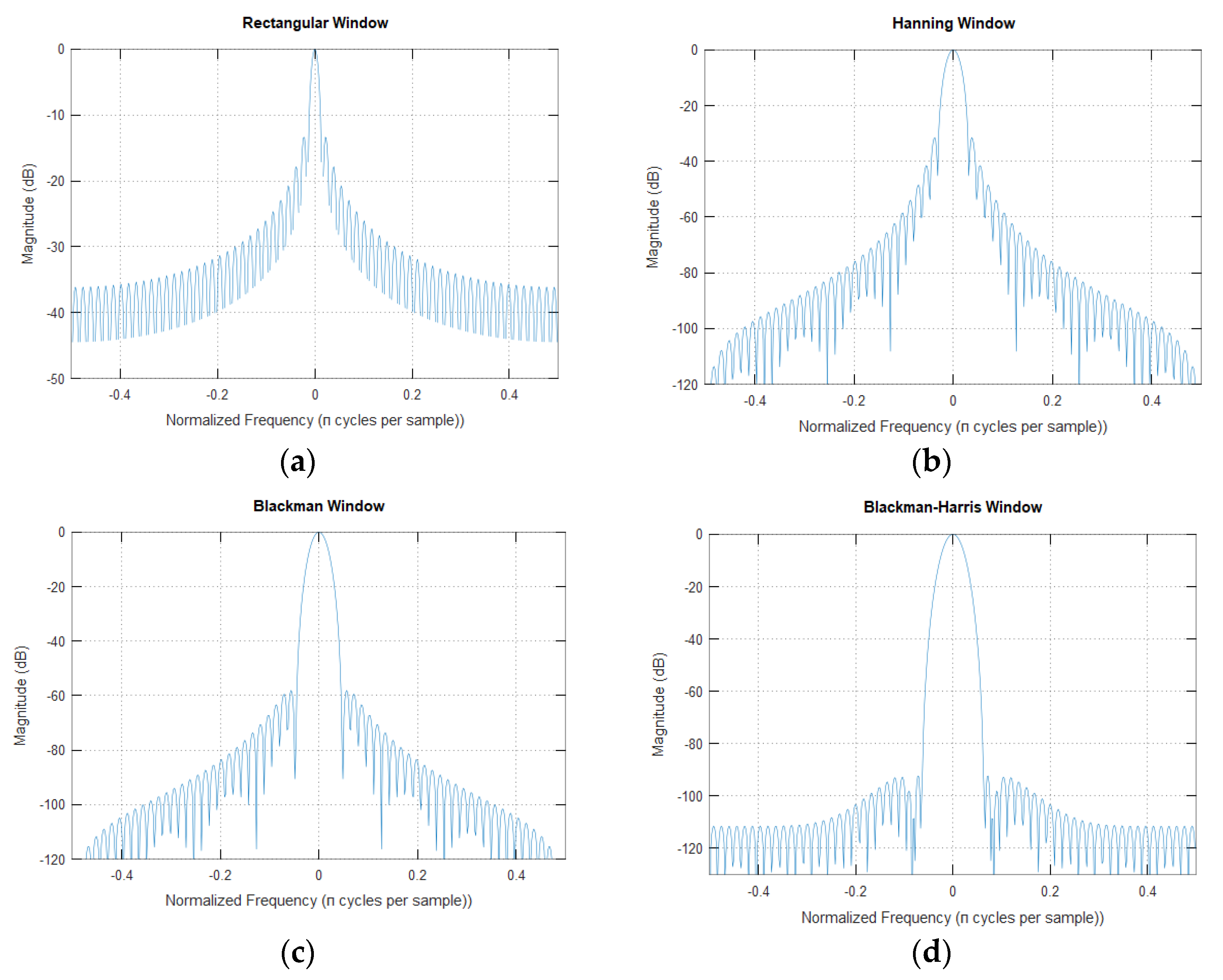
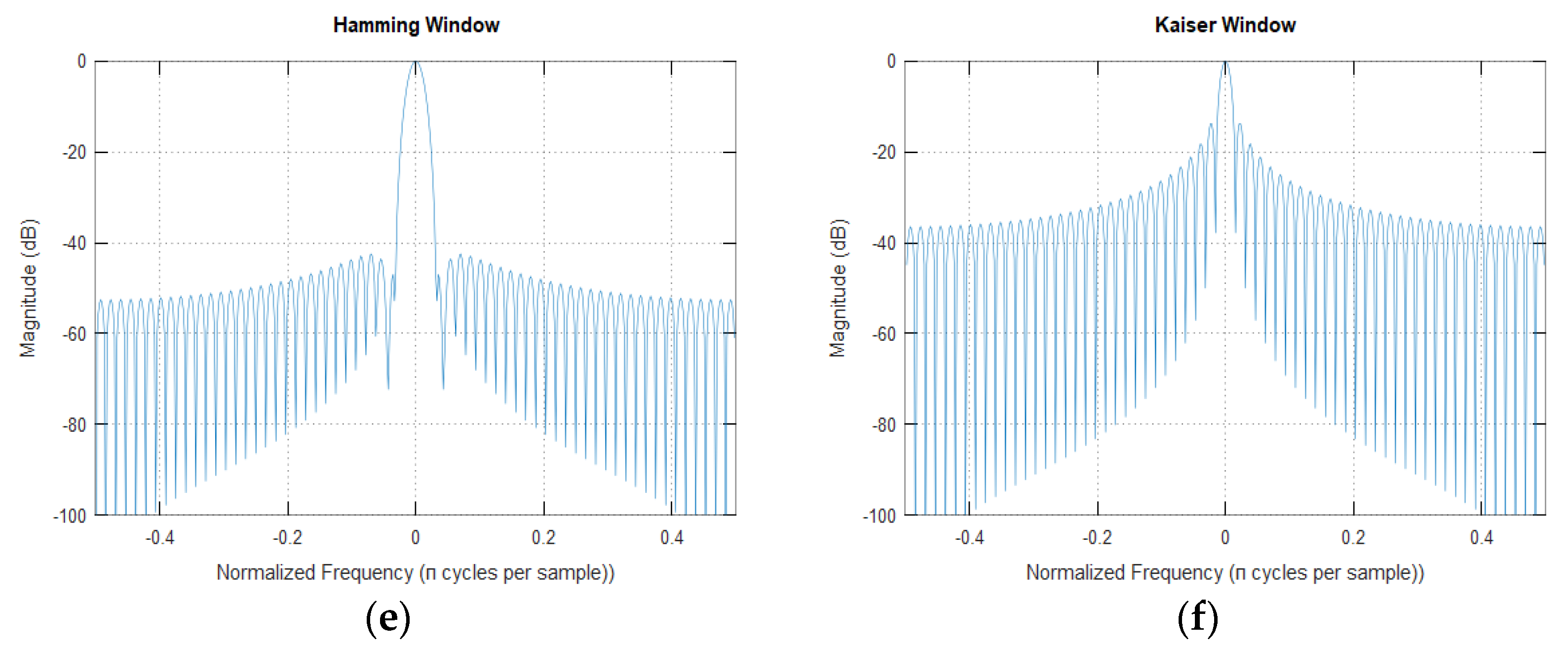
Figure 3 shows the spectrum of various types of windows which shows that the rectangular window has the lowest main lobe width while the Blackman Harris window has the widest main lobe.

Table 2. Properties of various window functions.

Window	$\mathit{w}\mathbf{\left(}\mathit{n}\mathbf{\right)}$	Width of the Main Lobe (3-dB BW) $\mathbf{\left(}\mathit{\pi }\frac{\mathbf{s}\mathbf{a}\mathbf{m}\mathbf{p}\mathbf{l}\mathbf{e}\mathbf{s}}{\mathbf{c}\mathbf{y}\mathbf{c}\mathbf{l}\mathbf{e}}\mathbf{\right)}$	Max Side Lobe Level (dB)	Side Lobe Roll-Off Rate (dB/Octave)
Rectangular	$\{\begin{array}{cc}1& 0\le n\le N\\ 0& \mathrm{Otherwise}\end{array}$	0.011719	−13.3	−6
Hanning	$\frac{1}{2}\left(1-\cos \left(\frac{2\pi n}{N}\right)\right), 0\le n\le N$	0.019531	−31.6	−18
Hamming	$0.54+0.46\cos \left(\frac{2\pi n}{N}\right), 0\le n\le N$	0.019531	−43.7	−6
Blackman	$0.42-0.5\cos \left(\frac{2\pi n}{N}\right)+0.08\left(\frac{4\pi n}{N}\right), 0\le n\le N$	0.023438	−58.2	−18
Blackman–Harris	$0.35875-0.48829\cos \left(\frac{2\pi n}{N}\right)$ $+0.14128\cos \left(\frac{4\pi n}{N}\right)-0.01168\cos \left(\frac{6\pi n}{N}\right)$	0.027344	−92.2	−6
Kaiser	$\frac{I_0\left[\beta \sqrt{1-{\left(1-\frac{2n}{N}\right)}^2}\right]}{I_0\left(\beta \right)}, 0\le n\le N$ ($\beta$ is a parameter that determines the tradeoff between main lobe width and side lobe levels)	0.011719	−14.7	−6

shows the various properties of these windows [11,14].

As discussed in Section 1, spectral leakage causes low power spectral components to be obscured especially when their power level is low. In the problem of estimating PIM from the PSD at the output of a nonlinear model, this is manifested as inability of the estimated PSD to show the PIM components at the IMD frequencies when the input power is low as PIM components usually have power levels of 100 dB less than the power of the main channel. In the following section, simulations of the PSD of the output a passive nonlinearity using various window functions are presented.

Simulation Results and Discussion:

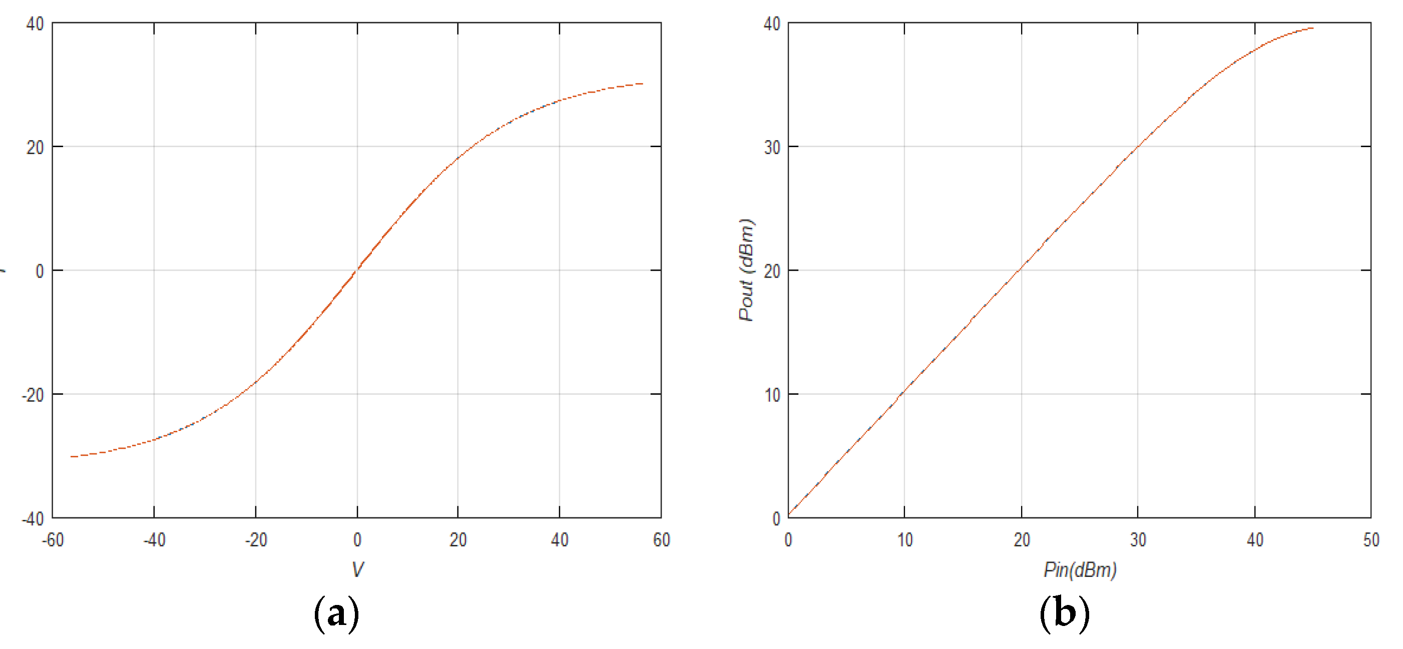
The theoretical concepts presented in the paper are verified by simulations results. The behavioral model used in the simulations is based on a hyper tangent function which has been shown in [18,19] to follow measured nonlinear I/V characteristics of a passive nonlinearity over an input power range of more than 30 dB. The hyper tangent function is given by 9

$$I\left(t\right)=g_0\left[1+k_1\tanh \left(k_{2}V\left(t\right)\right)\right]$$

(11)

where g₀, k₁ and k₂ are the model parameters which can be adjusted to fit a wide variety of nonlinear characteristics. Note that these characteristics can model the less than 3 dB/dB behavior of a passive nonlinearity by the proper selection of the model parameters. The passive nonlinearity in the simulations that will follow was generated using a hyper tangent model with parameters k₁ = 6 × 10⁻⁵, k₂ = 3 × 10⁻³ and g₀ = 1. Figure 4a shows the I/V characteristics of the hyperbolic tangent model and Figure 4b shows the input/output power characteristics of the model.

The input signal to the model was generated in Matlab and is based on the specifications of the Orthogonal Frequency Division Multiplexed (OFDM) signals that resemble LTE signals as shown in

Table 3. OFDM Signal Parameters.

No. of Sub-Carriers	1705
Modulation	16 QAM Constellation type: Gray
Pulse Shaping	Rectangular pulse
PAPR	10.8 dB
Input Power range	0 dBm to 35 dBm

[16]. The periodogram of the output of the passive nonlinearity in (10) was computed for an input that consists of two simulated OFDM signals with 20 MHz bandwidth each and a frequency separation of 100 MHz. The periodogram was estimated using different window functions. Note that, in order for the periodogram of the output of the nonlinearity to show the IMD components, the sampling frequency needs to be greater than the highest IMD component. For example, in order to show the 9th intermodulation component, the sampling frequency must be greater than $9{\omega }_0$.

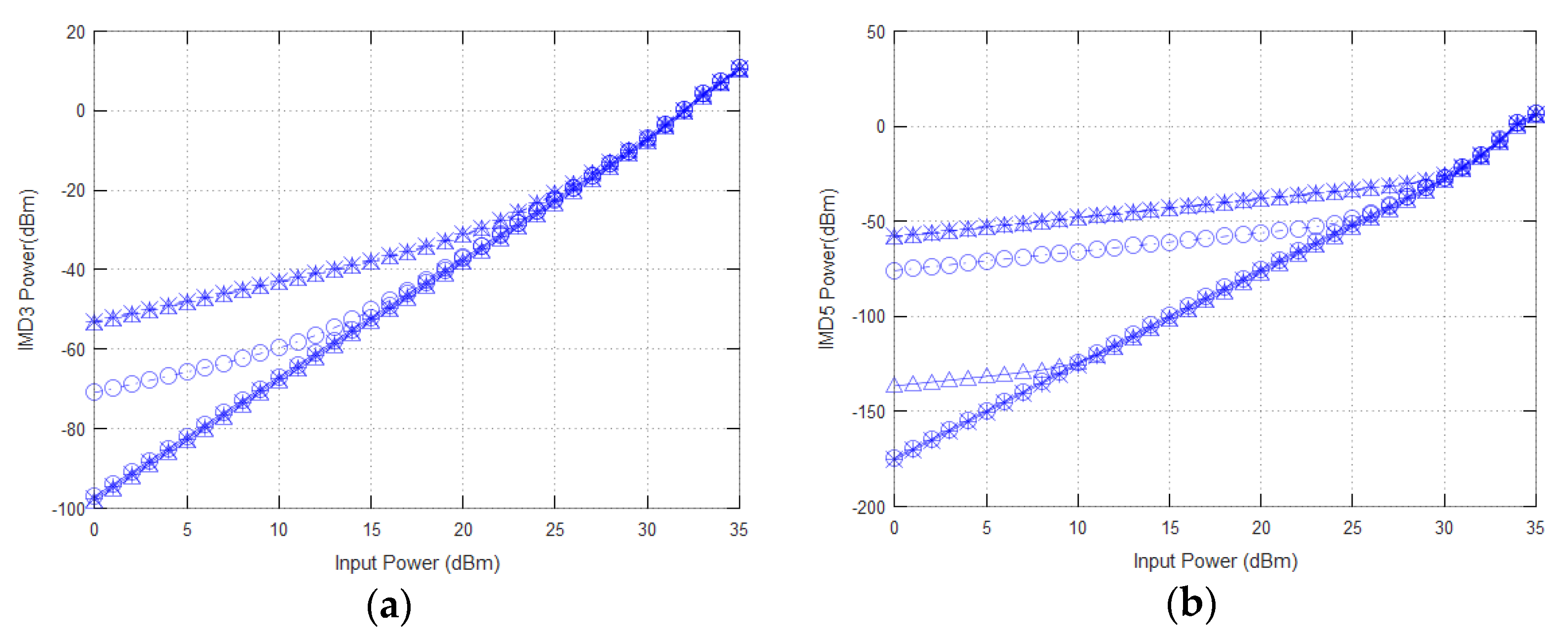
The simulation results include computing PIM distortion from the PSD of the output of the nonlinearity at various IMD frequencies and power levels. The power of the input signals is swept in a range of 0 to 35 dBm and the periodogram was computed at each power level. The power in the IMD components is computed within a bandwidth of 20 MHz. In order to study the effect of the intermodulation frequency on the prediction capability of the power spectral density with a given window function to predict PIM components, the frequency separation between the input carriers was swept and the passive IMD components were computed at various frequency separations and using different window functions.

4. Results

Figure 5 shows the PSD of the output of the nonlinear model for an input that consists of two OFDM signals separated by 100 MHz. The PSD was estimated using a periodogram with two window functions: a Hanning window and a rectangular window when the input power is much lower than the saturation point of the nonlinearity (Pin = 30 dBm). At this input power, the level of the IMD components is very low as compared to the main channel power. The figure clearly shows that with a rectangular window the periodogram only predicts the third order PIM component but fails to predict all higher order IMD components due to the severe spectral leakage. In contrast, a periodogram that uses a Hanning window predict all IMD components which have power levels as low as −200 dBm.

To analyze the effect of the window function on the capability of the PSD to predict PIM components, the periodogram was computed using the different window functions presented in Table 1 and with a frequency separation of 20 MHz between the two input carriers. The power of PIM at the IMD frequencies was calculated from the PSD within the same bandwidth of the input signal for various input power levels as shown in Figure 6a–d. The figures show the input power levels at which the periodogram (which uses a given window function) can predict the PIM power of all nonlinear orders.

The effect of frequency separation between the two carriers was also studied where the PSD of the periodogram of the output of the nonlinearity was simulated using different window functions at different frequency separations and, hence, different separation between IMD frequencies and the fundamental frequencies at a carrier power of 35 dBm as shown in Figure 7a–d.

5. Discussion

Table 4. IMD estimation using various window function.

	Pin = 0 dBm				Pin = 30 dBm
Window	IMD3	IMD5	IMD7	IMD9	IMD3	IMD5	IMD7	IMD9
Rectangular	−53	−58	−60.9	−62.8	−6.8	−25.7	−31.4	−33.7
Kaiser	−53.4	−58.3	−61.2	−63.1	−6.8	−25.8	−31.7	−34
Hamming	−70.9	−75.9	−78.8	−80.7	−7	−27.3	−43.7	−50.9
Hanning	−96.7	−174.4	−211	−218	−7	−27.3	−45.8	−64.7
Blackman	−97.5	−175.3	−219	−226	−7.4	−28	−46.8	−65.6
Blackman Harris	−98.1	−136.5	−139.4	−141	−7.8	−28.8	−47.9	−66.8

summarizes the results obtained from Figure 6a–d where it is shown that the Blackman and Blackman–Harris windows have best performance in predicting PIM components in comparison to other windows at all power levels and all orders of PIM. The table also shows that at low input power levels, Blackman window surpasses other window function in predicting all PIM component, while at high input power, the Blackman and the Blackman–Harris windows show a similar result in predicting PIM component. These results are consistent with the properties of the window function in Table 1 which shows that although the Blackman window has side lobe level (−58 dB) which is much higher than the Blackman Harris window, it has better performance than the Blackman Harris window for higher order IMD components. The reason for this is that although the Blackman Harris window has a better side lobe level performance (−92 dB), the Blackman window has a much higher roll-off rate of the side lobes (−18 dB/decade) especially when the frequency separation between the two input signals is small and hence, high frequency PIM components. On the other hand, at high input power level, the PIM components have a higher power level and hence, both windows have similar PIM prediction performance.

The results in Figure 7a–d show that for higher order PIM components (5th order and higher), the Blackman and Hanning windows provide the lowest IMD power and hence, the best PIM prediction capability regardless of the frequency separation. With other window functions, the figures show that the PIM level decreases with increasing the frequency separation between the carriers as a result of spectral leakage. These results comply of the properties of the different window functions in Table 1 where the Blackman and Hanning windows have the best side lobe roll of (−18 dB/decade), which means that the spectral leakage decreases rapidly with increasing frequency separation and hence, the PSD can better predict IMD components of all orders than other window functions. For the third order PIM component, Figure 7a shows that Hamming and Kaiser windows provide better prediction capability at high frequency separations and, at the same time, the worst PIM prediction capability at lower frequency separations. The reason for this is the low side lobe roll-off rate of these windows which results in higher spectral leakage at low frequencies. On the other hand, the Blackman and Hanning windows offer reasonable PIM prediction at all frequency separations, which make them better candidates for spectral estimation of PIM than the Hamming and Kaiser windows.

6. Conclusions

In this paper, prediction of PIM in carrier aggregated system from the output spectrum of a behavioral model of a passive nonlinearity has been studied. Since PIM components usually have a very low power levels, it has been shown that spectral leakage has a significant effect of the prediction capability of the PSD to identify PIM components. A detailed analysis and simulations of the impact of the choice of the window functions on prediction of PIM distortion has been presented. Since the frequency and the power of IMD frequencies depend on the frequency separation between the main channels and their power levels, it has been shown that accurate prediction of PIM components from the output PSD requires window functions that compromise the side lobe levels and the side lobe roll-off rates. The simulation results showed that, in principle, window functions that have high side lobe roll-off rates (Hanning and Blackman) offer better PIM prediction when IMD components are strong and distant from the main carrier (high frequency separation between the main carriers). On the other hand, window functions with low side lobe levels (Blackman and Blackman Harris) offer better prediction of PIM components when the IMD components are weak and close to the main carriers (low frequency separation between the main carriers).