Unsupervised Subcategory Domain Adaptive Network for 3D Object Detection in LiDAR

Abstract

Three-dimensional object detection based on the LiDAR point cloud plays an important role in autonomous driving. The point cloud distribution of the object varies greatly at different distances, observation angles, and occlusion levels. Besides, different types of LiDARs have different settings of projection angles, thus producing an entirely different point cloud distribution. Pre-trained models on the dataset with annotations may degrade on other datasets. In this paper, we propose a method for object detection using an unsupervised adaptive network, which does not require additional annotation data of the target domain. Our object detection adaptive network consists of a general object detection network, a global feature adaptation network, and a special subcategory instance adaptation network. We divide the source domain data into different subcategories and use a multi-label discriminator to assign labels dynamically to the target domain data. We evaluated our approach on the KITTI object benchmark and proved that the proposed unsupervised adaptive method could achieve a remarkable improvement in the adaptation capabilities.

1. Introduction

LiDAR-based 3D object detection is an important module for autonomous driving. Thanks to the great success of deep learning techniques and a large amount of annotated data, the detection performance has improved significantly in the past few years. However, in practice, we always find that a pre-trained object detection model may perform well on the original dataset, but the performance may degrade dramatically on other datasets. After analyzing the reasons for performance degradation, we attribute it to the different distribution of the point cloud in the source domain and the target domain.

For autonomous driving, the 3D point cloud is often generated by emitting and receiving laser rays to the environment from the center of the multi-channel LiDAR. Therefore, the point cloud distribution changes dramatically as the ranging distance increases. Besides, different types of LiDARs have different settings of projection angles, thus producing an entirely different point cloud distribution.

In this paper, we focus on the unsupervised domain adaptation algorithm that has the potential to overcome the dataset bias problem. This kind of algorithm aims to model the difference between the source domain and the target domain, and the models trained in the source domain implicitly take this difference into account, thus having the potential to perform well in the target domain.

In the task of object detection, the domain adaptation methods could be simply classified as global data adaptation methods and local instance adaptation methods. For the global data adaptation method, the goal is to minimize the whole gap between the source domain and the target domain, so the scene-level difference can be modeled. In contrast, local instance adaptation methods take the instance representation into account and help to reduce the local instance difference. In practice, these two types of approaches are usually combined for a more robust result. In Reference [1], the authors revealed the relationship between global and instance adaptation and trained two additional domain classifiers to enhance the performance of Faster RCNN. In Reference [2], the authors believe that the difference at the scene level may be too large for a perfect match; therefore, it proposes to combine the weak global alignment with the strong local alignment for object detection adaptation.

Recently, generative adversarial learning is also introduced to design domain adaptation algorithms. This kind of algorithm tries to minimize domain discrepancy through discriminators. This kind of algorithm has achieved great success for detecting objects in 2D image [3]. However, compared with 2D images, the objects in the 3D point cloud are characterized not only by their 3D position but also by the scale and 3D orientation. Therefore, a simple generative adversarial network (GAN) that confuses whether the object belongs to the source domain or the target domain may not be adequate. As previously mentioned, the point cloud in 3D varies a lot at different ranges or different observation angles; therefore, the objects should be better grouped into different subcategories. It is well known that the use of category labels can significantly improve the quality of the generated samples. LabelGAN [4] expands the generated samples with an additional category label. The generator of CatGAN [5] directly optimizes the entropy of the different sub-categories, so each generated sample will have a high degree of confidence for certain categories.

In this paper, we propose a novel unsupervised domain adaptation method for 3D object detection. The proposed approach combines global adaptation with local multiple subcategory adaptation. This algorithm aims to improve the object detection performance in the target domain without any additional labeled data. The proposed approach is a generic approach that could be used in conjunction with any deep learning-based object detection networks [6]. To enhance the performance, the 3D objects are divided into subcategories based on observation angle and object orientation. A multi-label discriminator is designed to classify these samples. The designed multi-label network can minimize the domain discrepancy at the instance level. Additionally, a global adaptation network is also designed to normalize the structure of the point cloud.

We evaluate our adaptation model on the KITTI benchmark [7]. Experimental results indicate that the proposed approach could obtain a remarkable improvement in the adaptation capabilities.

This paper is structured as follows: In Section 2, we review the related work. Section 3 shows the entire framework of our method and introduces the global adaptation network and subcategory instance adaptation network. In Section 4, the implementation details of our method are introduced. The qualitative and quantitative experiments on the KITTI benchmark are introduced in Section 5. Section 6 shows the ablation study of our method, and then the conclusions are given in Section 7.

2. Related Work

2.1. 3D Object Detection

3D object detection based on the LiDAR point cloud has always been a central task for autonomous driving. Depending on the representation approach for the LiDAR point cloud, existing approaches could be categorized into three categories: 3D voxel-based approach, 2D projected view-based approach, and point-based approach. A typical representation of point cloud is to discretize the 3D space into voxels, and a 3D convolutional neural network(CNN) could then be directly applied to the voxel. However, the 3D convolution [8] is considered to be a computationally expensive approach. To reduce the computational cost, the resolution of voxels has to be set to a relatively large value. To remedy this, Wang et al. [6] propose a cascaded network that subdivides the initial voxel into smaller voxels to increase the resolution. Sparse convolution [9,10] is another technique that has been used to accelerate the processing speed. It utilizes the sparsity of the point cloud, and only performed the convolution at locations where the data exists. To avoid the 3D convolution, some approaches are directly performed on the original point cloud [11,12,13] to extract point-wise features. The 3D point cloud could also be projected to the 2D image view [14,15], but some information might get lost after the projection. This paper aims to design a domain adaptation method that is applicable for all the different object detection approaches.

2.2. Unsupervised Domain Adaptation

Learning-based methods usually assume that the data characteristics on the training set and the testing set should be approximately the same; therefore, the model trained on the training set can be directly applied to the testing set. However, in practice, we sometimes find that the distribution of labeled training data and testing data are not the same. To tackle this problem, domain adaptation [16,17] approaches have been designed. They try to minimize the gap [18,19] between the source domain and the target domain, in hopes that the model trained in the source domain is still valid in the target domain. A typical method is to introduce an additional discrepancy loss in the training step to generate domain invariance features [20,21,22]. This approach is also known as the direct domain alignment approach. Other than the direct domain alignment, an indirect method called domain adversarial learning [23,24,25,26,27] has attracted increasing attention recently. In domain adversarial learning, a discriminator is trained to distinguish features of the source domain from the target domain, and a generator (backbone network) is simultaneously trained to fool the discriminator. This adversarial process helps to generate domain invariance features.

Although there has been a lot of research on domain adaptation for object detection, it is still a challenging task. Most of the previous works focus on image-based object detection. Adaptive Faster RCNN [1] combines global and local instance feature alignment and uses a gradient reversal layer [28] to train the adversarial network. Strong-weak Distribution Alignment [2] put the alignment focus on globally similar data and promote the consistency of local structural information. To deal with 3D point cloud, Rist et al. [29] proposed a cross-sensor domain adaptation method and demonstrated that the dense 3D voxels can better model sensor invariance features. SqueezeSegv2 [30] utilizes a simulation engine to generate labeled synthetic data. A model is then trained on the synthetic data and transferred to the real world. In Reference [31], the authors believe that the sparse point cloud is sampled from a dense surface. Therefore, a network is first trained to perform the surface completion. The recovered 3D surfaces serve as an intermediate representation for domain adaption.

3. Unsupervised Subcategory Domain Adaptive Network

3.1. Network Overview

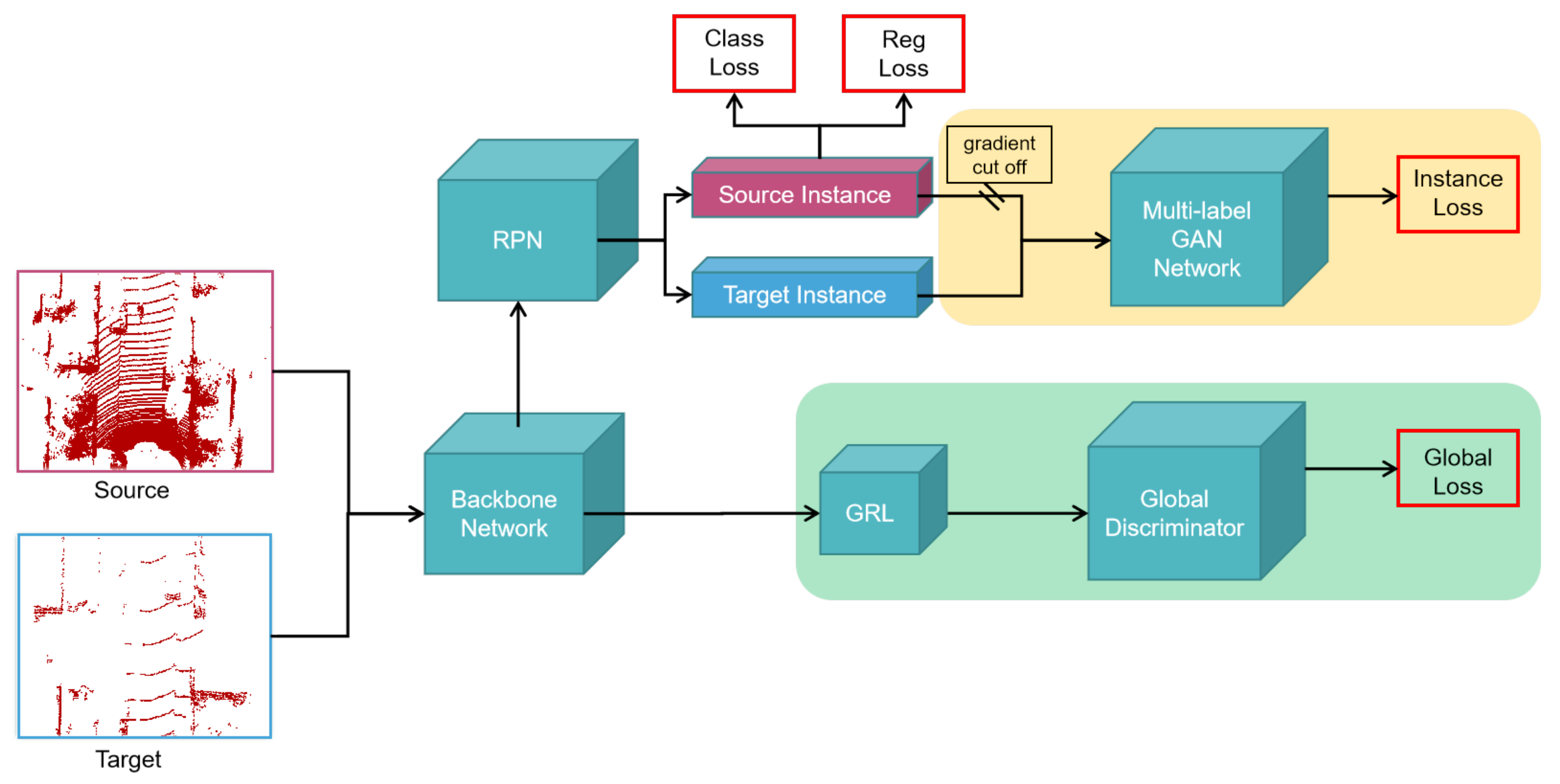
The architecture of the proposed subcategory adaptive network is illustrated in Figure 1. Our network consists of three modules, namely the object detection network, global feature adaptation network, and subcategory instance adaptation network. SCNET [6] is a 3D object detection network that considers both performance and efficiency. It is highly flexible and can be extended to other tasks. So, we choose SCNET as the object detection network. It is also the baseline model in this work. SCNET is a single-stage network consisting of a backbone network for global feature extraction and a region proposal network (RPN) for object classification. The global feature adaptation network is a generative adversarial network with a global domain discriminator. The subcategory instance adaptation network contains a multi-label discriminator.

In the training phase, data from the source domain and target domain simultaneously input to the object detection backbone network and share parameters. Only data from the source domain contains annotations. These annotations are utilized to tune the network parameters. The global feature adaptation network shares global features with the backbone network. To minimize domain shift, we use the gradient reverse layer (GRL) [28] to align the global features between the source and target domain. The global features then input to RPN for region extraction. To encourage domain adaptation at the subcategory level, a subcategory instance adaptation network is used to perform domain adaptation and local instance classification after region extraction. Especially, the multi-label discriminator is used to classify instances into different subcategories.

3.2. Global Feature Adaptation

A patch-based domain discriminator [32] is imposed to classify source domain and target domain. Specifically, the patch-based classifier makes a prediction for each data patch to eliminate the overall domain distribution mismatch. To reduce the difference between the two domains further, we reverse the gradient of the source domain and target domain to the backbone network through gradient reverse layer synchronously.

The global feature adaptation loss is expressed as

$$L_{global}=-\sum _i\left[y_{i}log{p}_i+(1-y_i)log(1-p_i)\right],$$

(1)

where $y_i\in [0,1]$ represents the label of patch i. $y_i=0$ indicates the source domain, and $y_i=1$ represents the target domain. $p_i$ is the prediction of domain classifier.

As an end-to-end network structure, we optimize the parameters of the domain discriminator to minimize the global feature classification loss and optimize the parameters of the backbone feature extraction network to maximize the loss. By optimizing the global loss, we obtain the domain invariant global features.

3.3. Subcategory Instance Adaptation

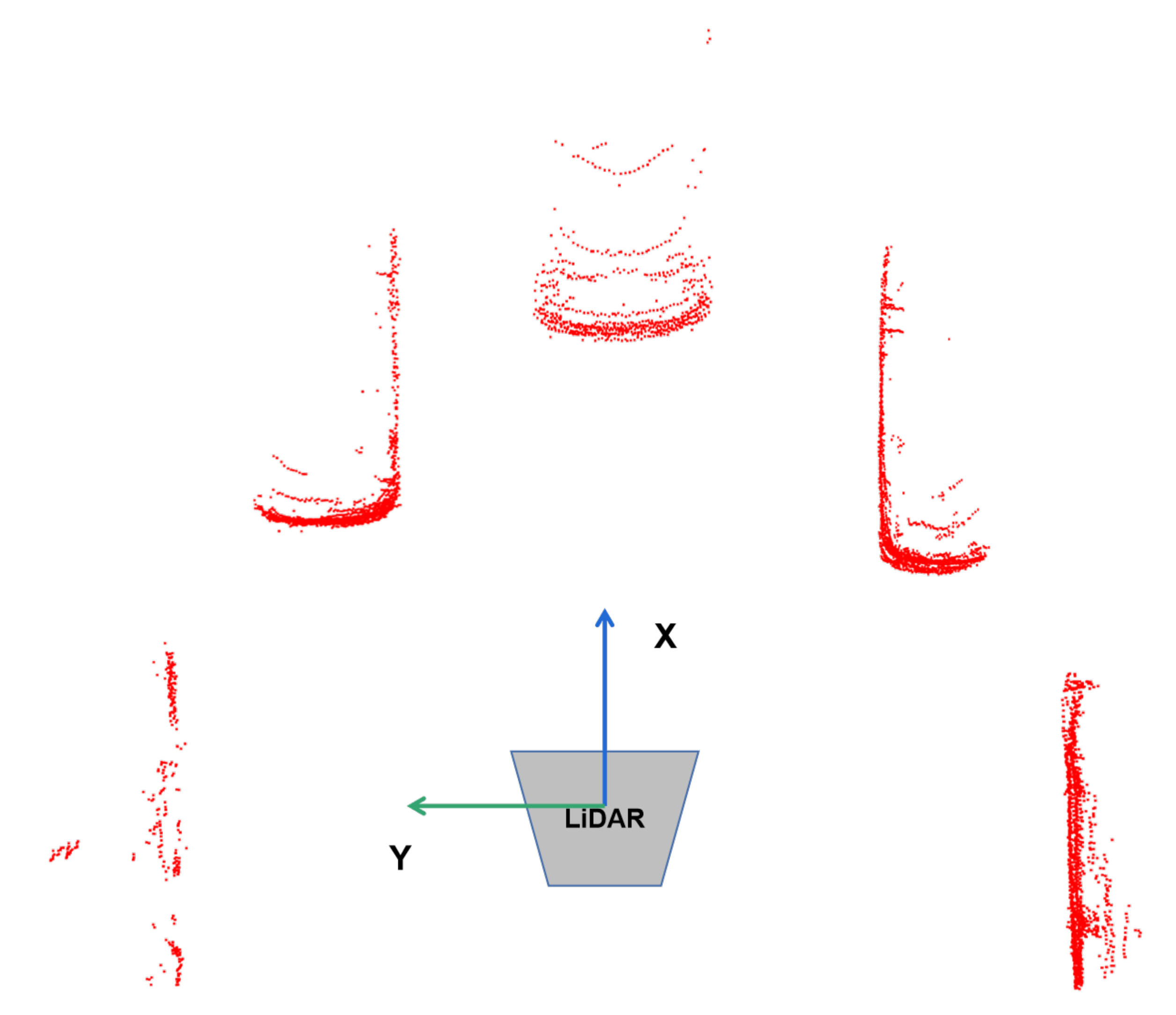
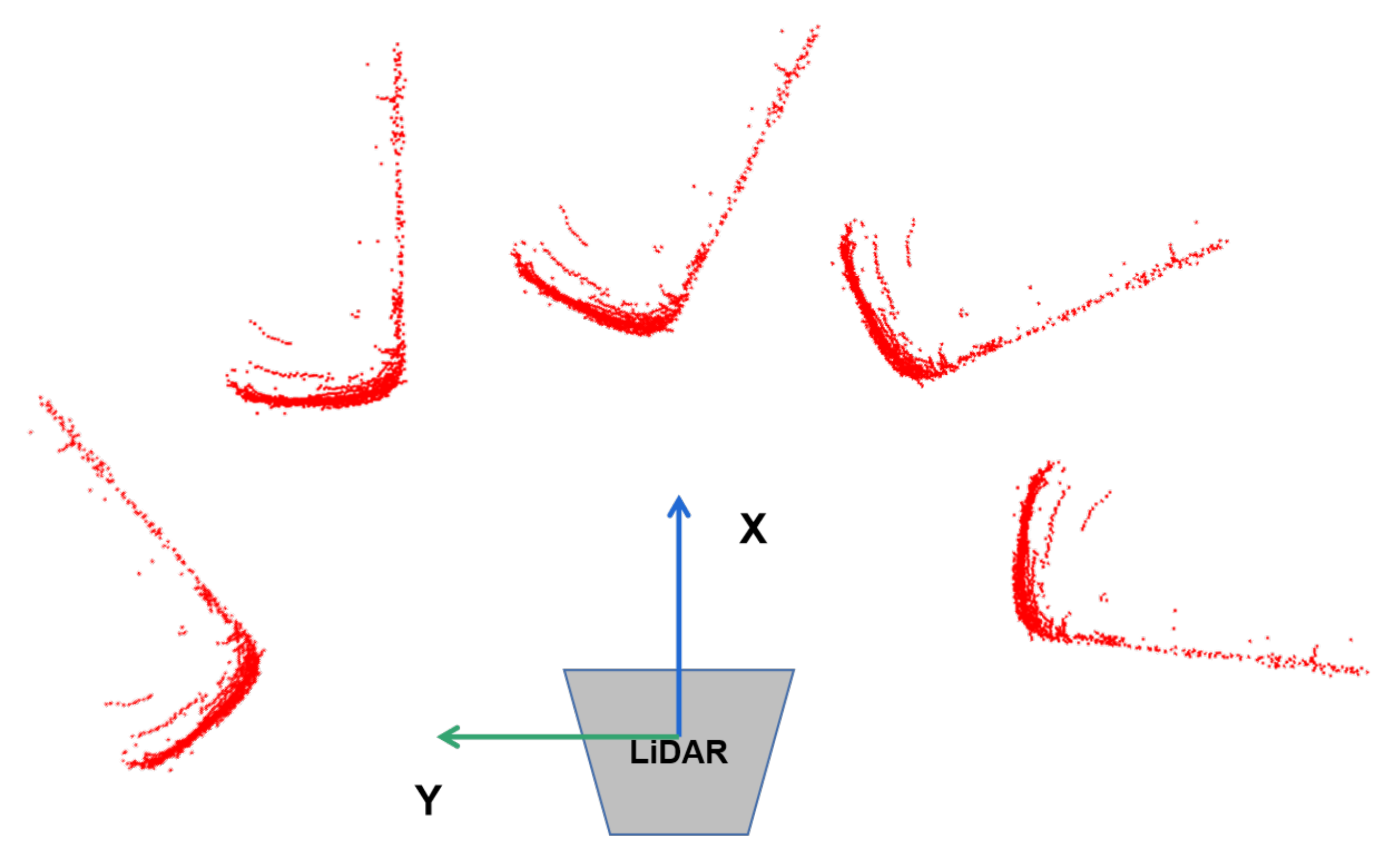
Subcategory Division. The structure of the 3D object in the LiDAR point cloud is diverse due to the difference in positions and orientation angles. Therefore, dividing all 3D objects into one category will lose the shape information within the category. As shown in Figure 2, due to the self-occlusion, objects with the same orientation angle might have completely different point cloud distribution. For the same observation angle, as shown in Figure 3, although the same part of the object can be observed, and the distribution of local point is the same, the whole point cloud is different in angle.

Because 3D point cloud describes the actual scale of the object, the distribution of the same object at different distances is consistent. As the distance increases, the point cloud density will gradually decrease. Objects with similar poses at different distances should have similar characteristics. The dense object can obtain more stable and complete representations. In the source domain, we choose complete objects without occlusion as the basic samples.

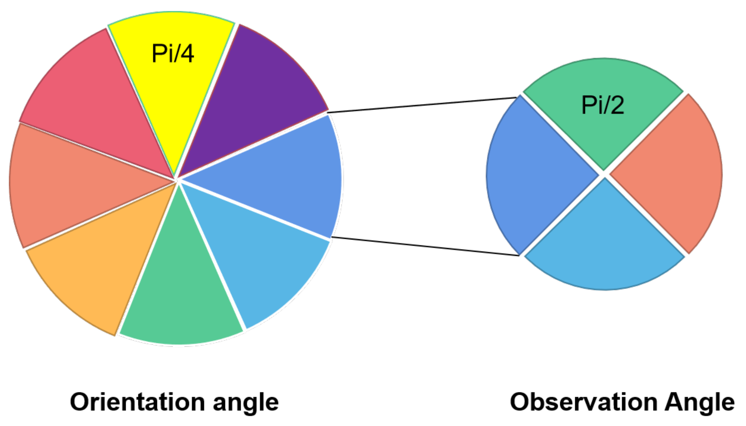
To minimize the intra-class difference, we classified each sample into different subcategories according to the observation angle and the object’s orientation angle.

The detail is shown in Figure 4. For these two angles, we divided them into N and M parts in the range of $[-\pi ,\pi ]$. Thus, the number of categories is $N\times M$.

Subcategory Instance Adaptation Network. To provide clear gradient guidance for the generator, the multi-label GAN trains the discriminator using the category labels on the source instance. The discriminator not only divides the source instance into the source domain with high confidence but also divides the instance into a subcategory. For the target domain instance, it is uncertain which existing category it is classified into, so the goal of the generator is to generate samples with higher confidence to classify it into a certain category and fool the discriminator. We divided all of the data into $K+1$ categories and $K+1$ is the label of the target domain instance. The loss function is defined as follows:

$$L_G={\mathbb{E}}_{(x,y)\sim G}\left[H(v\left(y\right),D\left(x\right))\right],$$

(2)

$$\begin{array}{c}\hfill L_D={\mathbb{E}}_{(x,y)\sim S_{data}}[H(v\left(y\right),D\left(x\right)]+\\ \hfill {\mathbb{E}}_{x\sim G}\left[H(v(K+1),D\left(x\right))\right],\end{array}$$

(3)

where $D_i\left(x\right)$ is the probability that x belongs to class i. $D\left(x\right)=\left[D_1\left(x\right),D_2\left(x\right),\dots ,D_{K+1}\left(x\right)\right]$, $v\left(y\right)=\left[v_1\left(y\right),v_2\left(y\right),\dots ,v_K\left(y\right)\right]$, $v_i\left(y\right)=1$ if $i=y$ else $v_i\left(y\right)=0$; H is the cross entropy.

For the discriminator, labeled source data should be correctly classified into one of the K categories, while the unlabeled target data should be correctly classified as belonging to the K + 1 category. For the generator, the target data should be classified into one of the K categories. AM-GAN [33] proposed a dynamic label method to evaluate the label of unsupervised data. As shown in Figure 5, all K + 1 categories can be treated equally. The discriminator shares the same features and simultaneously discriminates subcategories and domains. This method makes the category auxiliary classifier on the source domain participate in the adversarial training.

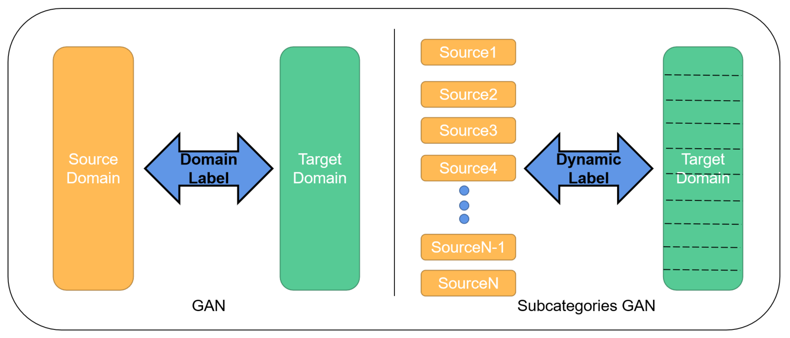
Based on the premise that each sample can correspond to a label, we assign a target class to each sample according to the currently estimated probability by the multi-label discriminator. The feature extracted by the discriminator can be then used for domain classification and category classification. Therefore, unlabeled data will automatically select the most probable category from the K categories with the highest probability. The difference between GAN and subcategories GAN can be seen in Figure 6.

$$y\left(x\right)\triangleq \underset{i\in 1,\dots ,K}{argmax}{D}_i\left(x\right).$$

(4)

Although the input of the multi-label GAN discriminator comes from the source data and the target data, we hope to optimize the performance of the target domain based on the source domain network. So, we cut off the gradient propagates through the source domain data to prevent the network from degrading the source domain features to align the cross-domain features.

3.4. Loss

Let $L_{det}$ denotes the loss of object detection network, which contains three different kinds of loss. The classification loss is used to evaluate the accuracy of the predicted category probability. The regression loss is used to learn the scale and posture of the object, and the direction loss can identify the direction of the object to enhance detection performance. The training loss of object detection network can be represented as:

$$L_{det}={\beta }_1{L}_{reg}+{\beta }_2{L}_{dir}+{\beta }_3{L}_{cls},$$

(5)

where ${\beta }_1, {\beta }_2, {\beta }_3$ are set to 2.0, 0.2, 1.0 according to SCNET.

The final training loss is defined as:

$$L=L_{det}+\lambda (L_{global}+L_{instance}),$$

(6)

where $\lambda$ is the loss weight to balance the detection loss and adaptation loss. The $L_{instance}$ is equal to the $L_G$. During inference, two adaptive networks can be removed, and only the object detection network with adapted weights is used.

4. Implementation

In this section, we introduce the implementation details of the network. We perform unsupervised domain adaptation in our experiments. The data consists of two parts: the source domain data with annotations and the target domain data without annotations.

SCNET [6] is chosen as the object detection framework. The structure of this network can be briefly divided into two steps: rasterization of unsorted point cloud and a regular backbone network for prediction and regression. SCNET adds an extra subdivision encoding network to enhance resolution. The original SCNET is trained on the source domain as the baseline without any adaptive operation. The results with different adaptive modules are reported in our experiments.

The network is trained with Stochastic Gradient Descent (SGD). The initial learning rate is 0.0002, and the decay weight is set to 0.8. The hyper-parameters are the same as the original SCNET. The trade-off parameter $\lambda$ is set as 0.1. All experiments are run on a computer equipped with GTX 1080Ti GPU and Intel i7 CPU@3GHZ.

In the KITTI dataset, we select point cloud data within the range of $[-3,1]\times [-40,40]\times [0,70.4]$ meters on the Z, Y, and X axes. The orientation angle is divided into 8 parts and the observation angle is also divided into 4 parts. Thus, the number of subcategories is 32.

In the initial training stage, the training of the discriminator should be emphasized. As the training continues, the training of the generator should gradually increase and eventually reach a balance with the discriminator. The parameter $\alpha$ in the GRL is used to adjust this balance. It is calculated as:

$$\alpha =\frac{0.2}{1+exp(-10·p)},$$

(7)

where p is defined as the ratio of the current iteration number to the total iteration number. So, $\alpha$ is a dynamic value that gradually changes from 0 to 0.2.

We evaluate the car detection performance using the KITTI evaluation protocols, where the IOU threshold is set to 0.7. The average precision (AP) is used to evaluate the performance. The same threshold is applied in both the bird’s eye view (BEV) and the 3D view.

5. Experiments

The KITTI Object benchmark contains 7481 training data. Following Reference [34], it is divided into a training subset of 3712 samples and a validation subset of 3769 samples. There are three different difficulty levels: easy, moderate, and hard. The difficulty levels account for different sizes, occlusions, and truncation, which are key factors influencing the detection results. We evaluate the performance both in the bird’s eyes view and 3D view.

Due to the scanning characteristics of the LiDAR, object samples in the near range are quite different from those far-away objects. Therefore, we treat the near range as the source domain and the far-away range as the target domain. The range threshold is set to 35.2 m. The annotations in the far-away range are removed to evaluate the unsupervised adaptation capability of the proposed approach.

As shown in

Table 1. The average precision (AP) of the object detection for different IOU values in the validation dataset.

Threshold	AP-BEV			AP-3D
	Easy	Moderate	Hard	Easy	Moderate	Hard
$IOU=0.7$	0.00	48.73	48.01	0.00	29.41	29.34
$IOU=0.5$	0.00	63.12	62.12	0.00	61.53	56.58

, we train our baseline object detection network on the source domain and evaluate it on the target domain with different IOU thresholds. It is observed that the performance is significantly enhanced when the IOU threshold is reduced from 0.7 to 0.5. This result indicates that the object detector could detect far-away objects well, but it encounters difficulties to accurately localize them.

The performance of different adaptive modules is shown in

Table 2. The object detection performance of our method. G denotes the global feature adaptation, and L denotes the subcategories instance adaptation.

Methods	AP-BEV			AP-3D
	Easy	Moderate	Hard	Easy	Moderate	Hard
SCNET	0.00	48.73	48.01	0.00	29.41	29.34
SCNET (G)	9.09	52.48	51.43	0.00	31.50	30.66
SCNET (L)	2.27	54.91	51.65	2.27	32.30	31.15
SCNET (G + L)	4.55	56.25	53.01	4.55	32.62	31.89

. Compared with the basic network, the proposed method achieves $+3.75\%$ and $+2.09\%$ gains on BEV and 3D object detection using the global adaptation module. The proposed method also achieves $+6.18\%$ and $2.89\%$ gains by using the instance adaptation module only. This proves that global and instance-level adaptation modules can effectively reduce the domain shift. Combining these two modules, the final gains are $+7.52$ and $+3.21$, respectively, at the moderate level. The results proved the necessity of reducing global and local domain shifts.

The division of difficulty level takes into account the image size, occlusion, and truncation of the object. Because their image height is lower than the easy level judgment standard, objects in the far-away range are rarely classified as easy level. The small amount of easy objects in the far-away range explains the huge fluctuations in detection performance at the easy level.

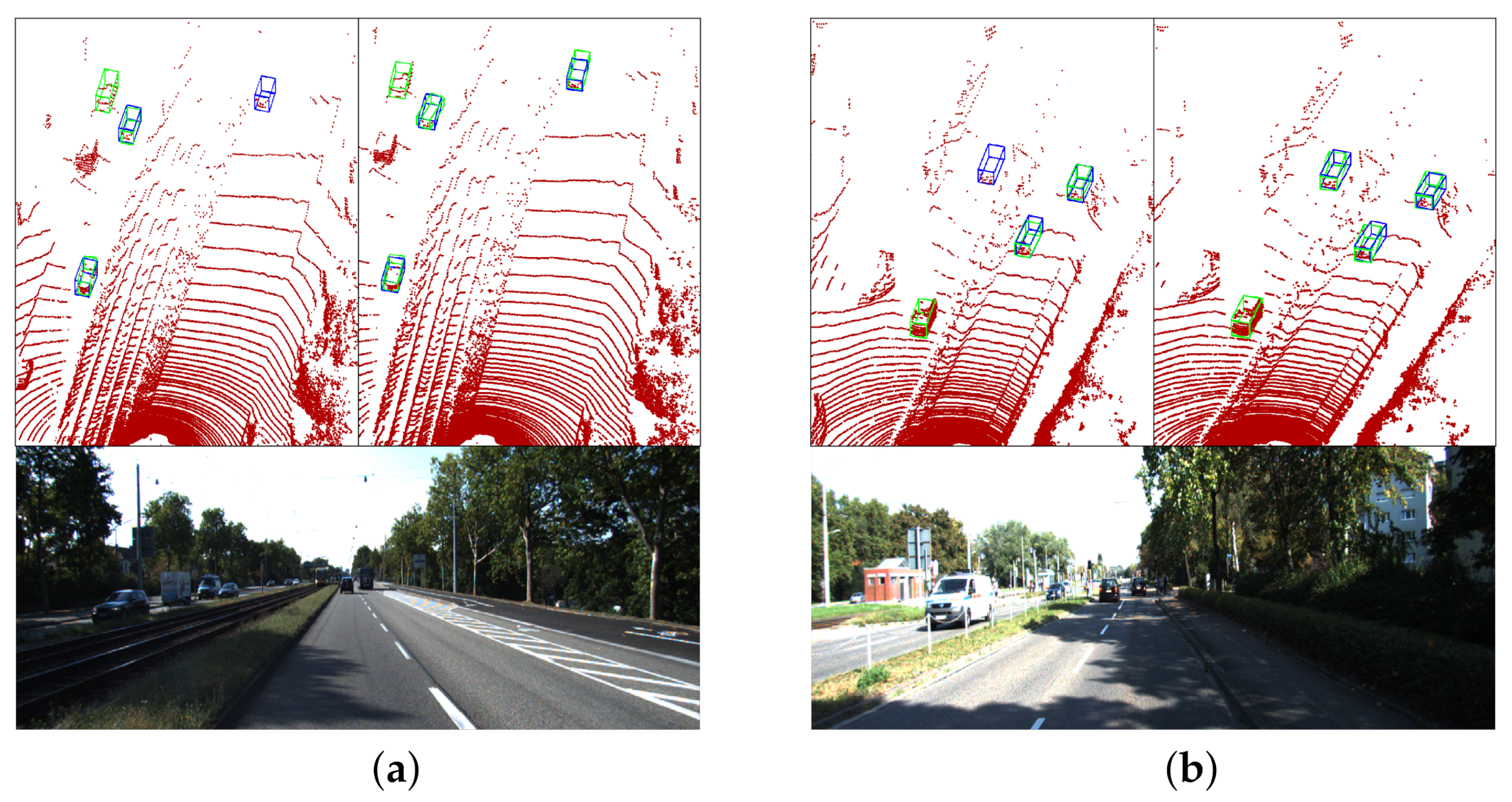
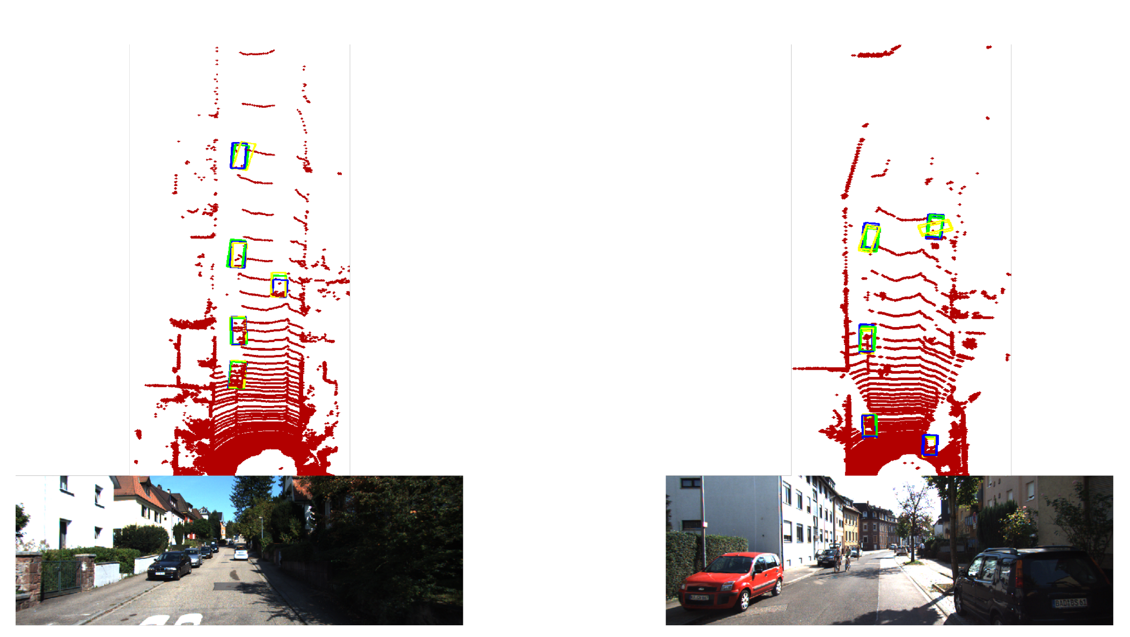
Some qualitative results are shown in Figure 7 and Figure 8. From Figure 7, it is observed that the proposed adaptive network increases the recall rate of distant objects. Figure 8 shows a typical orientation error under a correct classification result. It is clearly shown that our proposed adaptive network can improve the orientation estimation.

6. Ablation Study

6.1. Adaptation via GAN and Multi-Label GAN

We also compare the general GAN and our multi-label GAN. The key difference is object correspondence. GAN utilizes the discriminator to distinguish the target domain from the source domain, and then uses the generator to adjust the target domain to reduce the domain difference. This is a typical data transferring method similar to the global adaptation. GAN does not take full advantage of the instance characteristics, but only enhances the global adaptation. The multi-label GAN divides the source domain data into multiple subcategories and estimates the dynamic label of the target domain data based on the discriminator. In this way, the categories are expanded from two categories to multiple categories. A discriminator shares parameters to perform category classification and domain classification at the same time.

In this experiment, two instance adaptation results are listed in

Table 3. Performance of the object detection for different type of GAN.

Methods	AP-BEV			AP-3D
	Easy	Moderate	Hard	Easy	Moderate	Hard
GAN	4.55	55.24	52.34	4.55	31.79	30.82
Multiple categories GAN	4.55	56.25	53.01	4.55	32.62	31.89

. From the results, it is observed that GAN does improve the detection performance in the target domain, but inferior to the multi-label GAN with subcategories. With different poses, the distribution of the 3D point cloud has a greater change than the image. The result shows that the multiple subcategories division of the source domain data can provide more effective information in transfer learning compared with treating it as one category.

6.2. Cross-Device Adaptation

We have explored the range adaptation of homogeneous data. Here, we show experiments on the dissimilar domain adaptation from 64-channel data to 32-channel LiDAR data. The vertical resolution to determine the object density is one of the main parameters of LiDAR. Generally, there are significant performance differences between models trained with different line numbers. We construct a new 32-channel point cloud data based on the KITTI dataset. We uniformly sample the origin 64-channel point cloud data through the vertical angle. We use it as the target domain data to be learned. The new 32-channel dataset contains 3712 samples for training and 3769 samples for validation.

The new 32-channel dataset has the same number of frames as the origin 64-channel data, but the input order of the two domain data is random, so the two data will not be aligned during the training process. The range of both data is $[-3,1]\times [-40,40]\times [0,70.4]$ m.

Table 4. Bird’s eye view (BEV) detection performance on adaptation from 64-channel data to 32-channel data.

Methods	Full-Range (0–70.4 m)			Far-Range (35.2–70.4 m)
	Easy	Moderate	Hard	Easy	Moderate	Hard
SCNET	89.10	78.84	78.62	4.55	46.89	45.01
SCNET(G + L)	89.61	80.01	79.03	4.55	52.43	46.76

and

Table 5. Three-dimensional detection performance on adaptation from 64-channel data to 32-channel data.

Methods	Full-Range (0–70.4 m)			Far-Range (35.2–70.4 m)
	Easy	Moderate	Hard	Easy	Moderate	Hard
SCNET	78.19	67.00	64.78	0	22.49	21.72
SCNET(G + L)	84.00	68.22	66.19	0	26.57	25.53

present our results on BEV and 3D. The results show that the method that combines global adaptation and local instance adaptation gets the best performance. Compared with BEV object detection, the performance of 3D object detection has been greatly improved. Since the performance of 3D object detection has been greatly affected by domain shift, the adaptive method can improve more performance. Similarly, long-distance data that is greatly affected by the domain shift will also be improved than overall data.

6.3. Subcategories Division

We divide the object into different subcategories according to the orientation angle and observation angle. The orientation angle represents the local orientation and the observation angle combines local direction and position information. The combination of global and local information is sufficient to describe the change in point cloud distribution.

The number of the subcategories is critical to the multiple categories classification. We divide the orientation angle and observation angle into 4 parts and 8 parts, respectively. In total, we have four combinations, namely $4\times 4$, $4\times 8$, $8\times 4$, and $8\times 8$. The results under different settings are shown in

Table 6. Performance of the object detection for different subcategory divisions.

Methods	AP-BEV			AP-3D
	Easy	Moderate	Hard	Easy	Moderate	Hard
4 × 4	4.55	55.77	52.30	4.55	32.18	31.49
4 × 8	3.03	55.96	52.31	3.03	32.46	31.83
8 × 4	4.55	56.25	53.01	4.55	32.62	31.89
8 × 8	4.55	55.77	52.30	4.55	32.18	31.49

. It is observed that the combination of $8\times 4$ gets the best result. In theory, as the resolution increases, the performance gradually improves. The experiment shows a similar trend. When the angle resolution is set to $4\times 4$, the performance slightly outperforms GAN, and the best performance is achieved at resolution $8\times 4$. But the larger resolution $8\times 8$ could not get better performance. The possible reason is that the discriminator could hardly distinguish too many subcategories.

7. Conclusions

In this paper, we have proposed an unsupervised model adaptation method for object detection in the 3D point cloud. We use adversarial global feature adaptation and subcategory instance adaptation to achieve the cross-domain adaptation. We consider the variability of the point cloud and divide source domain data into multiple subcategories based on the annotations. The subcategory instance adaptation network uses a multi-label GAN network to assign labels dynamically to target domain data. Our method has successfully applied 3D point cloud subcategory information to reduce the discrepancy between source and target domain data. We evaluated our adaptation method on the KITTI dataset and demonstrated the combination of global feature adaptation and subcategory instance adaptation can significantly improve the performance of the unsupervised adaptation model.

References

- Chen, Y.; Li, W.; Sakaridis, C.; Dai, D.; Van Gool, L. Domain adaptive faster r-cnn for object detection in the wild. In Proceedings of the IEEE conference on computer vision and pattern recognition, Salt Lake City, UT, USA, 18–23 June 2018; pp. 3339–3348. [Google Scholar]
- Saito, K.; Ushiku, Y.; Harada, T.; Saenko, K. Strong-weak distribution alignment for adaptive object detection. In Proceedings of the IEEE Conference on Computer Vision and Pattern Recognition, Long Beach, CA, USA, 15–20 June 2019; pp. 6956–6965. [Google Scholar]
- Wang, M.; Deng, W. Deep visual domain adaptation: A survey. Neurocomputing 2018, 312, 135–153. [Google Scholar] [CrossRef]
- Salimans, T.; Goodfellow, I.; Zaremba, W.; Cheung, V.; Radford, A.; Chen, X. Improved techniques for training gans. arXiv 2016, arXiv:1606.03498. [Google Scholar]
- Springenberg, J.T. Unsupervised and semi-supervised learning with categorical generative adversarial networks. arXiv 2015, arXiv:1511.06390. [Google Scholar]
- Wang, Z.; Fu, H.; Wang, L.; Xiao, L.; Dai, B. SCNet: Subdivision coding network for object detection based on 3D point cloud. IEEE Access 2019, 7, 120449–120462. [Google Scholar] [CrossRef]
- Geiger, A.; Lenz, P.; Urtasun, R. Are we ready for Autonomous Driving? The KITTI Vision Benchmark Suite. In Proceedings of the Conference on Computer Vision and Pattern Recognition (CVPR), Providence, RI, USA, 16–21 June 2012. [Google Scholar]
- Zhou, Y.; Tuzel, O. Voxelnet: End-to-end learning for point cloud based 3D object detection. In Proceedings of the IEEE Conference on Computer Vision and Pattern Recognition, Salt Lake City, UT, USA, 18–23 June 2018; pp. 4490–4499. [Google Scholar]
- Graham, B.; van der Maaten, L. Submanifold sparse convolutional networks. arXiv 2017, arXiv:1706.01307. [Google Scholar]
- Yan, Y.; Mao, Y.; Li, B. SECOND: Sparsely Embedded Convolutional Detection. Sensors 2018, 18, 3337. [Google Scholar] [CrossRef] [PubMed]
- Qi, C.R.; Liu, W.; Wu, C.; Su, H.; Guibas, L.J. Frustum pointnets for 3D object detection from rgb-d data. In Proceedings of the IEEE Conference on Computer Vision and Pattern Recognition, Salt Lake City, UT, USA, 18–23 June 2018; pp. 918–927. [Google Scholar]
- Charles, R.Q.; Hao, S.; Mo, K.; Guibas, L.J. PointNet: Deep Learning on Point Sets for 3D Classification and Segmentation. In Proceedings of the IEEE Conference on Computer Vision and Pattern Recognition, Honolulu, HI, USA, 21–26 July 2017. [Google Scholar]
- Qi, C.R.; Yi, L.; Su, H.; Guibas, L.J. PointNet++: Deep Hierarchical Feature Learning on Point Sets in a Metric Space. arXiv 2017, arXiv:1706.02413. [Google Scholar]
- Chen, X.; Ma, H.; Wan, J.; Li, B.; Xia, T. Multi-view 3d object detection network for autonomous driving. In Proceedings of the 2017 IEEE Conference on Computer Vision and Pattern Recognition (CVPR), Honolulu, HI, USA, 21–26 July 2017; Volume 1, p. 3. [Google Scholar]
- Ku, J.; Mozifian, M.; Lee, J.; Harakeh, A.; Waslander, S.L. Joint 3D proposal generation and object detection from view aggregation. In Proceedings of the 2018 IEEE/RSJ International Conference on Intelligent Robots and Systems (IROS), Madrid, Spain, 1–5 October 2018; pp. 1–8. [Google Scholar]
- Csurka, G. Domain Adaptation in Computer Vision Applications; Springer: Berlin/Heidelberg, Germany, 2017. [Google Scholar]
- Patel, V.M.; Gopalan, R.; Li, R.; Chellappa, R. Visual domain adaptation: A survey of recent advances. IEEE Signal Process. Mag. 2015, 32, 53–69. [Google Scholar] [CrossRef]
- Long, M.; Cao, Y.; Wang, J.; Jordan, M. Learning transferable features with deep adaptation networks. In Proceedings of the International Conference on Machine Learning, Lille, France, 6–11 July 2015; pp. 97–105. [Google Scholar]
- Li, D.; Yang, Y.; Song, Y.Z.; Hospedales, T.M. Deeper, broader and artier domain generalization. In Proceedings of the IEEE International Conference on Computer Vision, Venice, Italy, 22–29 October 2017; pp. 5542–5550. [Google Scholar]
- Ghifary, M.; Kleijn, W.B.; Zhang, M.; Balduzzi, D.; Li, W. Deep reconstruction-classification networks for unsupervised domain adaptation. In Proceedings of the European Conference on Computer Vision, Amsterdam, The Netherlands, 8–16 October 2016; Springer: Berlin/Heidelberg, Germany, 2016; pp. 597–613. [Google Scholar]
- Sener, O.; Song, H.O.; Saxena, A.; Savarese, S. Learning transferrable representations for unsupervised domain adaptation. In Proceedings of the 30th International Conference on Neural Information Processing Systems, Barcelona, Spain, 5–10 December 2016; pp. 2118–2126. [Google Scholar]
- Motiian, S.; Piccirilli, M.; Adjeroh, D.A.; Doretto, G. Unified deep supervised domain adaptation and generalization. In Proceedings of the IEEE International Conference on Computer Vision, Venice, Italy, 22–29 October 2017; pp. 5715–5725. [Google Scholar]
- Ganin, Y.; Ustinova, E.; Ajakan, H.; Germain, P.; Larochelle, H.; Laviolette, F.; Marchand, M.; Lempitsky, V. Domain-Adversarial Training of Neural Networks; Guide to 3D Vision Computation; Springer: Cham, Switzerland, 2017; Volume 17, pp. 189–209. [Google Scholar] [CrossRef]
- Tzeng, E.; Hoffman, J.; Saenko, K.; Darrell, T. Adversarial discriminative domain adaptation. In Proceedings of the IEEE Conference on Computer Vision and Pattern Recognition, Honolulu, HI, USA, 21–26 July 2017; pp. 7167–7176. [Google Scholar]
- Shrivastava, A.; Pfister, T.; Tuzel, O.; Susskind, J.; Wang, W.; Webb, R. Learning from simulated and unsupervised images through adversarial training. In Proceedings of the IEEE Conference on Computer Vision and Pattern Recognition, Honolulu, HI, USA, 21–26 July 2017; pp. 2107–2116. [Google Scholar]
- Hoffman, J.; Tzeng, E.; Park, T.; Zhu, J.Y.; Isola, P.; Saenko, K.; Efros, A.; Darrell, T. Cycada: Cycle-consistent adversarial domain adaptation. In Proceedings of the International Conference on Machine Learning, Stockholm Sweden, 10–15 July 2018; pp. 1989–1998. [Google Scholar]
- Bousmalis, K.; Silberman, N.; Dohan, D.; Erhan, D.; Krishnan, D. Unsupervised pixel-level domain adaptation with generative adversarial networks. In Proceedings of the IEEE Conference on Computer Vision and Pattern Recognition, Honolulu, HI, USA, 21–26 July 2017; pp. 3722–3731. [Google Scholar]
- Ganin, Y.; Lempitsky, V. Unsupervised domain adaptation by backpropagation. In Proceedings of the International Conference on Machine Learning, Lille, France, 7–9 July 2015; pp. 1180–1189. [Google Scholar]
- Rist, C.B.; Enzweiler, M.; Gavrila, D.M. Cross-sensor deep domain adaptation for LiDAR detection and segmentation. In Proceedings of the 2019 IEEE Intelligent Vehicles Symposium (IV), Paris, France, 9–12 June 2019; pp. 1535–1542. [Google Scholar]
- Wu, B.; Zhou, X.; Zhao, S.; Yue, X.; Keutzer, K. Squeezesegv2: Improved model structure and unsupervised domain adaptation for road-object segmentation from a lidar point cloud. In Proceedings of the 2019 International Conference on Robotics and Automation (ICRA), Montreal, QC, USA, 20–24 May 2019; pp. 4376–4382. [Google Scholar]
- Yi, L.; Gong, B.; Funkhouser, T. Complete & label: A domain adaptation approach to semantic segmentation of LiDAR point clouds. arXiv 2020, arXiv:2007.08488. [Google Scholar]
- Johnson, J.; Alahi, A.; Fei-Fei, L. Perceptual losses for real-time style transfer and super-resolution. In Proceedings of the European Conference on Computer Vision, Amsterdam, The Netherlands, 8–16 October 2016; Springer: Berlin/Heidelberg, Germany, 2016; pp. 694–711. [Google Scholar]
- Zhou, Z.; Cai, H.; Rong, S.; Song, Y.; Ren, K.; Zhang, W.; Yu, Y.; Wang, J. Activation maximization generative adversarial nets. arXiv 2017, arXiv:1703.02000. [Google Scholar]
- Chen, X.; Kundu, K.; Zhu, Y.; Berneshawi, A.G.; Ma, H.; Fidler, S.; Urtasun, R. 3d object proposals for accurate object class detection. In Proceedings of the Advances in Neural Information Processing Systems, Montreal, QC, USA, 7–12 December 2015; pp. 424–432. [Google Scholar]
Figure 1.
An overview of our subcategory domain adaptive network: We perform model adaptation from two aspects, the global features and subcategory instance features. Both are trained by generative adversarial rules. Different domain data extract features through the same backbone network and an region proposal network (RPN) is used to extract instance features. The instance discriminator is designed as a multi-label generative adversarial network (GAN) network for subcategory classification.
Figure 2.
Point cloud distribution with the same orientation angle. In different locations, the distribution of point cloud is completely different.
Figure 3.
Point cloud distribution with the same observation angle. The local point cloud distribution is the same, but the rotation angle is different.
Figure 4.
Orientation angle and observation angle are selected as the factors for classification. The orientation angle is divided into N parts, and the observation angle is divided into M parts. The total number of categories is .
Figure 5.
Multi-label GAN. When training discriminator, the Source data is divided into K categories, and the target data is classified as the K + 1. And, for the generator, the target is classified into one of the K categories.
Figure 6.
GAN uses the domain label to divide the data into two categories. The multi-label GAN uses the source domain labels to divided the data into N subcategories, while the target domain data uses corresponding dynamic labels to reduce the difference with the source domain subcategories.
Figure 7.
The qualitative results for recall rate. We compare the performance of original method and proposed adaptive method in two scenes (a,b). In each subfigure, the top-left picture is the original results and the top-right picture is our results. The bottom picture is the image corresponding to the point cloud. The blue bounding boxes represent the ground truth boxes, and the green bounding boxes are the detection results. The results show that the proposed adaptive network can detect some objects that cannot be detected by the original method, thereby improving the recall rate of distant objects.
Figure 8.
The qualitative results for orientation error. For better visualization, we put the results of the original network and proposed adaptive network together. The blue bounding boxes represent the ground truth box. The yellow bounding boxes represent the original result, and the green bounding boxes represent the results of the adaptive network. The result shows a typical direction error under a correct classification result. The direction of the green boxes is closer to the blue ground truth box, and the direction of the yellow bounding box is quite different from the blue bounding box. Our proposed adaptive network can improve the orientation accuracy.