Abstract
Haze is a natural distortion to the real-life images due to the specific weather conditions. This distortion limits the perceptual fidelity, as well as information integrity, of a given image. Image dehazing for the observed images is a complicated task because of its ill-posed nature. This study offers the Deep-Dehaze network to retrieve haze-free images. Given an input, the proposed architecture uses four feature extraction modules to perform nonlinear feature extraction. We improvise the traditional U-Net architecture and the residual network to design our architecture. We also introduce the spatial-edge loss function that enables our system to achieve better performance than that for the typical and loss function. Unlike other learning-based approaches, our network does not use any fusion connection for image dehazing. By training the image translation and dehazing network in an end-to-end manner, we can obtain better effects of both image translation and dehazing. Experimental results on synthetic and real-world images demonstrate that our model performs favorably against the state-of-the-art dehazing algorithms. We trained our network in an end-to-end manner and validated it on natural and synthetic hazy datasets. Our method shows favorable results on these datasets without any post-processing in contrast to the traditional approach.
1. Introduction
Haze is usually an atmospheric phenomenon that appears due to the atmospheric absorption and scattering of light reflected by the objects in the scene. A typical camera captures the images of outdoor scenes with a tiny aperture, with the quality varying depending on the amount of light from the scene passing through the aperture. Due to fume, fog, mist, cloud in the ambient, image sensors capture reflection information in conjunction with haze. Various computer vision algorithms, such as object detection and tracking, are suitable for use under haze-free scene radiance. Hence, image dehazing is compulsory to ensure haze-consistent performance in many vision-based tasks [1].
In the past two decades, there has been significant progress in image dehazing research that was initiated by investigating techniques for the estimation of depth information. The introduction of Koschmeider’s atmospheric scattering model [2] provided a key breakthrough, and the solution of this model has been used by most of the state-of-the-art methods that seek transmission map estimation and atmospheric light separately to recover the dehazed image as described by:
Here, is the degraded hazy image, denotes the transmission map, is the haze-free image, and A is the global atmospheric light. An light incoming to the camera sensor is not independent of the transmission map that explicitly controls the sensor’s visual quality. A functional model of a hazy image fundamentally contains two components, namely, the transmission information and the scattered atmospheric light. Both of these jointly comprise the hazy image in theory. Assuming the atmospheric light A is homogeneous, the expression for the transmission map is , where represents the attenuation coefficient of the atmosphere and is the depth information of the scene. Many studies have been proposed based upon Equation (1) and the previously mentioned assumption for homogeneous distribution. We can generalize these studies into two classes of prior information-based methods [3,4,5,6,7,8] and learning-based method [9,10,11,12,13]. The methods that explored the transmission map are based on the estimation of the parameters of atmospheric scattering by utilizing priors, such as dark channel prior [6], color attenuation prior [14], and haze line prior [15,16,17,18]. By contrast, few works have focused on the estimation of the atmospheric light [19,20,21,22]. In the next section, we discuss on the previous and current trends in image dehazing [23,24,25,26,27,28,29,30,31,32,33,34,35,36,37,38,39,40,41,42,43,44,45,46,47,48].
In this study, we used an end-to-end approach to perform single image dehazing. Our network at the first stage takes the hazy input image without any preprocessing. This image is Then, used as input into four different feature extraction blocks to extract the hazy information from the image. The four feature extraction blocks are as follows: Residual-U-Net (Res-U-net) with two entirely different filter properties, conventional residual block, and sequential residual block. In our Res-U-net, we utilize only one residual connection for the U-Net architecture. Moreover, this residual connection is a global residual connection that adds the input image with the extracted feature at the end of the network. This connection is in contrast to the widely practiced local residual U-Net architecture. This study is an extension of the approach of [45].
We perform 15 continuous convolution operations upon the input image for the conventional residual block, followed by a global residual connection. We only use the ReLU activation function in our residual block. We do not use any batch normalization in the residual block because normalization introduces a detrimental effect in regression-based learning. For our sequential-residual block, we concatenate the outputs from the residual blocks. Then, a simple convolution operation upon the concatenated tensor gives us the desired features. At this stage, the feature blocks have collected all of the essential features for subtraction from the input image. Following the subtraction, we concatenate the results together into a single tensor. A final convolution operation upon this tensor gives us the desired haze-free image.
We can summarize the overall contributions of our study as follows:
(a) Our Deep-Dehaze network uses the end-to-end property for dehazing of hazy input images. The proposed Deep-Dehaze system achieves state-of-the-art performances through the cooperation of four different feature extraction modules.
(b) In this work, we propose a sequential-residual module for feature extraction that outperforms the traditional residual block, dense block, and residual-attention block.
(c) The Res-U-net used in this work uses only one global residual connection. Due to this improvement of U-Net, our Res-U-Net outperforms the original U-Net-based module.
(d) Finally, we improve the use of the usual loss function by utilizing it for both the spatial and edge domains. This loss function helps our network to retrieve the fine details without using any fusion or gated fusion operation. Additionally, our reconstructed outputs are free from the burning effect unlike the outputs obtained by the prior-based approaches.
The rest of the paper is organized in the usual manner. The next section focuses on related works for the reconstruction of dehazed images. Then, we explain the network architecture and present relevant figures. Then, we compare our performance with other dehazing methods on various datasets, with the conclusions given in the final section.
2. Related Works
Image dehazing methods generally face several challenges, such as smoothed regions, protection of the edges without blurring, preservation of textures, and destruction through artifacts. A bulk of the recent advances in the image dehazing tasks are properly described in References [43,48]. The earliest dehazing method was to extract the scene depth of a single image of scenes captured in scattering media in the presence of the atmospheric effect [22]. Nayar-Narashiman [18,19] later proposed three different algorithms by using the dichromatic scattering model to estimate the depth of the hazy image. Despite sharing the same atmospheric light color, two images from the same scene contain different colors of direct transmission. Based on this theory, Narasimhan-Nayar [18,19] uses multiple gray or colored images of the scene captured in different haze density by extending their previous dichromatic scattering model. They estimated the scene structure by introducing the contrast restoration of iso-depth regions, atmospheric light estimation, and contrast restoration. Due to the direct transmission’s insignificant transition, observed light information suffers from fidelity degradation. Therefore, Oakley and Bu (2007) have assumed transmission light to be constant over the entire single image. They mentioned that the mean pixel intensity of the entire image is proportional to the standard deviation [20]. Tan et al., (2008) also assumed a smooth layer of transmission light through maximization of the local contrasts of the input image [21]. Fatal et al. [22] recover Equation (1) and estimate the scene’s albedo. Fatal et al. infers as the medium transmission that can describe the portion of the camera-reachable non-scattered light. They [21,22] proposed the Markov Random Field and independent component analysis (ICA), respectively, without adding any geometrical information. However, these methods cannot be used in real-time applications because of unexpected results with enhanced scene contrasts and some halos near depth discontinuities in various scenes.
Moreover, the environmental images based on remote sensing systems also suffer from atmospheric haze effects. A layer of clouds and aerosol contaminates these images captured by separate multi-spectral imaging sensors, such as Thematic Mapper. Addressing these issues, Chavez et al. (1988) proposed the dark-object subtraction method by subtracting a constant value from the darkest object in the scene [23]. Later, Zhang et al. [24] refined this method by calculating the haze-optimized transformation. Du et al. [25] eliminated the haze effects by corrupting the high-resolution satellite images into a different spatial spectrum and utilized the frequencies of the spectrum for haze removal.
Lately, researchers have focused on histogram equalization and gamma correction to ignore the spatial relations. This family of methods proposed that tone mapping can be another technique for general contrast enhancement because it depends only on pixel values. In 1997, Larson et al. [26] described a tone production operator for high-dynamic-range images. However, this method fails due to variation of the optical thickness of the haze across the image. Later, Laplacian pyramid [27], wavelet decomposition [28], and multi-scale bilateral filter [29] were used to amplify the local variations in the pixel intensity. These methods amplify the high-band image components multiplicatively for the given image. This amplification is due to the multiplicative and additive nature of the haze and results in poor fidelity.
Due to the decaying effect on color attenuation and color distortion, researchers concentrated on deep learning approaches and have achieved remarkable success in this field. Methods, such as DCNN, GAN, adversarial CNN, and unsupervised algorithms, have achieved considerable development in dehazing tasks. In contrast to the conventional physical-based haze removal approaches, these processes do not use any assumptions or priors. The multiscale CNN [9] was the first to remove the images by focusing on balance and contrast enhancement. They have utilized a coarse-scale and fine-scale subnetworks to learn the mapping between hazy images and their corresponding transmission maps. Another transmission map estimation network, Dehaze Net [30], uses a trainable model, adding feature extraction and nonlinear regression layers to estimate the transmission map. In addition to the existing approaches, AOD-Net [31] is the first end-to-end trainable image dehazing model where all of the parameters are updated through L1 minimization. This paper claims that an accurate transmission medium map does not directly measure or minimize the reconstruction distortion. As a result, it increases the sub-optimal restoration quality. AOD-Net was built on a different assumption and proposed a method of calculating a linear transformation to integrate both the transmission function and the atmospheric light. PFFNet, a variant of U-Net, learns the complex nonlinear transformation function in an end-to-end manner from the haze-affected images [32].
Similar to ResNet, DenseNet can scale hundreds of layers and connect two layers with the same feature-map size directly. Applying DenseNet, Densely Connected Neural Network (DCNN) [33] estimates the transmission map by introducing an edge-preserving loss function. Y-Net also introduces an encoder-decoder architecture next to the wavelet-based loss function. Here, they divide the input images into different sized patches with different frequencies and scales to learn the most discriminative features. The generic model-agnostic CNN (GMAN) learns to capture the haze structures in images and restores the clear images without referring to the atmospheric scattering model [33]. This encoder-decoder based architecture can solve the issues, such as color darkening and excessive edge sharpening. The Disentangled Dehazing network (DDN) [34] provides a novel perceptual dehazing to recover the scene radiance, transmission map, and global atmosphere using three generators jointly. For unsupervised layer decomposition of a single image, Double-DIP extends the theory of the “Deep Image Prior (DIP)” [35]. It introduces a robust unified framework to capture the low-level statistics of a single natural image. A fast deep multi-patch hierarchical network restores the non-homogenous hazed image by aggregating multiple patches’ features from different distinct sections of the hazed image [36]. Reference [47] achieves better performance by incorporating high-frequency and low-frequency features and used ResNet family architecture for their work.
General adversarial networks (GANs) also have popularized information synthesis for image style transformation. Haze removal can also be viewed as the task of transferring images from the hazy domain to the haze-free domain. Even though the GAN framework faces several challenges, such as mode collapse, training stability, and a sizeable computational budget, many different approaches have been developed to mitigate these issues [43,44,45]. A general adversarial network (FFDNet) is the fast and flexible adversarial denoising method of spatially variant noise removal by specifying a non-uniform noise level map [37]. Enhancing Cycle GAN, Cycle-Dehaze approaches a formulation that improves the quality of textual information by combining cycle-consistency and perceptual losses [38]. Instead of the typical cross-entropy based loss, Conditional Wasserstein GAN learns the probability distribution of a clear image concerning the haze-effected image using the Wessertian loss function. This particular method also uses a gradient penalty for improving the Lipschitz constraint [39]. Researchers have also used the GAN framework to estimate the transmission map by combining or replacing different CNNs as a subnetwork. Conditional GAN explicitly estimates the transmission map by replacing U-Net with the Tiramisu model [40]. CCGAN represents a classification-driven conditional generative adversarial network as a subnetwork by combining a dehazing sub-network (DNet) and a classification subnetwork (CNet) and optimizes them jointly [41]. DHSGAN proposes an end-to-end adversarial network to learn the underlying distribution of the clean images [42]. Reference [46] utilizes the U-Net-family GAN architecture to reconstruct crisper output for the given image and achieves state-of-the-art performance.
3. Network Details
As shown in Figure 1, our network learns the nonlinear relationship between the hazy input image and the output image. In this work, we focus on the design of smaller sub-networks for learning sophisticated features from the given input image. The included sub-networks allow our end-to-end network to learn image features, spatial properties, and haze patterns for the given input. We present the necessary description of these sub-modules below.
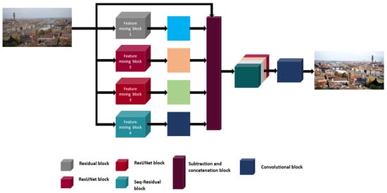
Figure 1.
The above diagram shows a schematic of the proposed Deep dehaze network. First, the hazy input image is fed into the four feature extraction blocks. These blocks extract the haze information from the input image. Then, these features are subtracted from the input image. The four different resultants are concatenated, and concatenation is followed by a convolution operation. This convolution operation provides the final output dehazed picture. Here, different colors for the Res-U-net module indicates different numbers of filter parameters.
In the original Unet architecture, the authors implement the autoencoder’s reflection at the core of their model. Autoencoder encodes the given image and seeks to reconstruct it as faithfully as possible. The Unet study extended this approach through the concatenation block. In the decoding part of the Unet, they have augmented each layer with a concatenation from the previous corresponding encoding layer. In essence, this property acts similar to a resnet architecture; here, concatenation returns the previous features instead of the previous gradients. The proposed Res-U-net block differs from the original Unet architecture by a single global residual connection. Established Unet with residual connections includes skipping links for every layer. These links allow the network to learn better than the original Unet architecture. The number of the channels increases for Unet after each pooling operation exponentially increases the skip connections at each layer. To reduce this increase, we use a single global skip connection for our Unet base architecture Figure 2. We have observed better performance for the Unet with a global skip connection. In our end-to-end Deep-Dehaze network, we have used two Res-U-net blocks for spatial feature learning. For the first Res-U-net, the channel increment starts from 32, and for the second, the number of channels increases exponentially from 16.
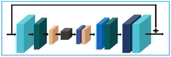
Figure 2.
Res-U-net module for our network.
Our residual block Figure 3 follows the typical design flow. We have included the skip connection to learn the spatial haze patterns from the given input. It is well-known that the residual connection can attain the underlying nonlinear relation between the input and the output image. For this reason, in ill-posed computer vision problems, the residual module is a popular choice. In our residual block, we have used 15 consecutive convolution operation before the skip connection. After learning the haze patterns at 15 layers, we have added the input image to the end of the module. For this module, we use 32 filters from the second convolution layer to the 14th layer. For the first layer and the last layer, we have used three channels. Our kernel width is 7 for each layer in the residual module.
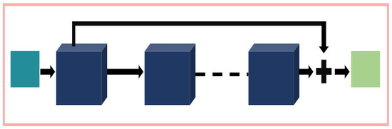
Figure 3.
Residual module for our network.
The proposed Seq-Residual block Figure 4 is the simple extension of the typical residual block, as described above. In this module, we have used three consecutive residual blocks, with one individual convolution operation after each residual block. Then, we have concatenated the residual blocks into a single tensor for the global feature learning. For each res blocks, we have used different kernel widths. Our kernel sizes are 3, 5, and 7. For the individual convolution operation, the kernel width is 3. At the final stage, we perform the last convolution operation to extract the global feature information of the concatenated tensor.
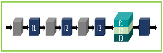
Figure 4.
Seq-Residual module for our network.
After extracting the desired features using the modules mentioned above, we perform the subtraction operation between the hazy input image and each module’s output. Then, we concatenate all of the results into a single tensor. This subtraction is the proposed network’s fundamental property because four sub-networks learn the corresponding heterogeneous feature distribution. The concatenation of these four diverse subtraction blocks contains the sporadic intermediate haze-free feature distribution. In other words, this concatenated tensor contains multiscale spatial information, inter-pixel relationship, and transmission light features. A final convolution operation upon this tensor completes our network’s single image dehazing task. It is reasonable for ill-posed computer vision problems to choose the loss function from the regression loss family. In our work, we focus on designing a suitable regression loss function to extract the best possible features from the given image space distribution. The following sub-section describes the proposed loss function in detail.
Loss Function
Mean-square error (MSE) or norm minimization is standard in the machine learning community for regression tasks. Even though the use of MSE loss is well-established, it is not free of pitfalls. For instance, when the convolution network involves image quality, is unable to correlate with image quality as effectively as a human observer. This is because during the use of the loss function is based on several assumptions. First and foremost, the use of assumes that the impact of noise is independent of the image’s local characteristics. On the other hand, the Human Visual System (HVS) is more sensitive to local luminance, color variation, contrast, and structure. Neural networks used for image-restoration-related tasks such as denoising, deblurring, demosaicking, and super-resolution always focus on tuning the network’s architecture.
Since vision-based regression tasks involve faithful reconstruction of the given image, the loss layer’s architecture is vital. Compared to the loss function, the loss function can be a preferable option due to the outlier treatment of these loss functions. In the presence of an outlier, the network takes a heavier penalty if the incorporated loss function is the mean-square error (MSE). Both and are preferable to find good minima. As mentioned above, is more robust for outliers than the loss function. Therefore, is preferable to the loss function due to the outlier scenario found in most neural networks. Experience shows that PSNR, SSIM, or MSSIM loss in conjunction with the MSE can reach a desirable solution, but these findings are specific to the dataset and the network design. In summary, MAE or mean-absolute error function does not square the error in contrast to the MSE and shows better convexity in practice; therefore, we focus on the MAE loss family to design our network’s loss function.
We use a combination of the loss function for the spatial and edge domains for our network. Usually, the system approximates the clean image from the given corrupted image based on a nonlinear relationship. Therefore, the performance of the network varies from image to image. Moreover, the spatial complexity of the given image makes this approximation more challenging. For this reason, the resultant image often contains less inter-pixel variance than the ground truth image. In other words, the reconstructed image is more likely to be the smoothed-out version of the original image. We use the loss function for both the edge and the spatial domains to address this problem. In the loss layer, we have used TensorFlow edge extractor function to obtain the edge information from the running batch of the images. We augmented the loss value from both of these in a weighted manner to constitute our proposed loss function. Our choice of weights is and for the spatial domain and the edge domain, respectively. We have set these weights empirically. Thus, we have achieved a sharper image compared to the traditional loss function. The proposed loss function is given by:
Here, is the loss function for the spatial domain and is the loss function for the edge domain. The loss function is given by:
In the above equation, is the ith value from the n samples, and is the network’s predicted value. The choice of the weights in equation 2 is obtained based on empirical evidence. The following section contains a detailed analysis of the results for our proposed network.
4. Result Analysis
Many datasets are available for training the deep learning network to perform image dehazing tasks. In our previous work, we used the RESIDE dataset for single image dehazing. We selected three subsets of the RESIDE dataset. They are the indoor training set, the outdoor training set, and the synthetic testing set. For validation, we used the indoor and outdoor validation set from the RESIDE dataset. We chose to use DIV2K dataset due to its versatility and high-resolution quality. Of course, we synthesized a hazy dataset out of the DIV2K through synthetic haze augmentation. For synthetic haze validation, we also used the validation set from the DIV2k dataset.
Both RESIDE and DIV2K dataset are publicly available. We used 10,000 images from the RESIDE dataset and 700 images from the DIV2K dataset for our overall training procedure. For the extreme dehazing performance, we used the dataset curated by Ancuti et al. [24]. This dataset contains extremely hazy images with their respective ground truths.
For our training setup, we kept the original training structure. We used the following training setup for our network. We sample our training images into 128 by 128 patches to reduce the training complexity. For our scheme, we use the Keras framework to design the dehazing network. For the ADAM optimizer, we keep the usual training parameter. We train the Deep-Dehaze network with the batch size of 16.
We compare to the results obtained using a new method [3] along with three previous methods. The methods chosen for comparison are fusion-based dehazing [3], Dark channel prior [6], Non-local prior [15], and All-in-one dehazing net [30]. We used the PSNR, SSIM, and MSE metrics to quantitatively characterize the performance of these methods.
The synthetic dataset from the RESIDE validation, DIV2k validation, and the extreme dehaze validation dataset from the Ancuti et al. [24] also contain the ground truth images. Figure 5 and Figure 6 shows the visual comparison between the method proposed in the study and the above-mentioned methods. In Figure 7, we present the comparative analysis for extreme dehazing. The left column of Figure 6 contains the input hazy image. This demonstration shows the side-by-side comparison of the single image dehazing performance. In the rightmost column, we see the dehazing performance for the dark channel prior [13]. As observed from the image, a dark channel prior helps the user to effectively remove the haze from the given image. However, the method faces the challenge of the burning-effect that is common for the usual dehazing methods. Due to the burning-effect, many dehazing schemes reduce the overall light information, decreasing the vital details. This method also reconstructs the given input image with an unnatural contrast, degrading the total fidelity of the input image.
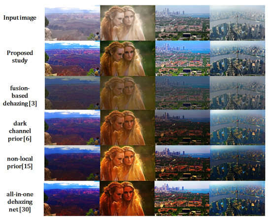
Figure 5.
Visual comparison study for our network. From top to below, input image, proposed study, Reprinted from [3,6,15,30].
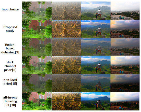
Figure 6.
Visual comparison between proposed study and the selected studies for more hazy images. From top to below, input image, proposed study, Reprinted from [3,6,15,30].
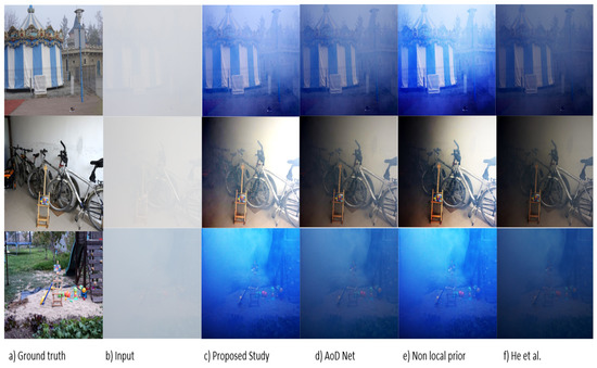
Figure 7.
Example of the extreme single image dehazing operation.
Figure 5 and Figure 6 show the results of the ablation study for our network. Perceptually, our network can reconstruct the haze-free images with superior contrast and brightness. For example, in Figure 5, our reconstruction of the women’s image shows the associated background most precisely. By contrast, AOD-Net has removed the haze properly but suffers from over contrast enhancement. In Figure 6, the image on the rightmost column is challenging. According to the graphical demonstration, our method can reconstruct the sky information precisely compared to the other studies. On the other hand, their reconstruction tends to blur the extracted sky region or distributed contrast poorly. Again, on the leftmost side, the wall image is one of the most widely used images in image dehazing studies. Our reconstruction of the input hazy images shows that the wall’s hazes are almost entirely eliminated compared to the other studies. However, for the extreme dataset challenge, our performance remains almost the same as before. This is due to the challenges within the domain adaptation of the deep learning studies. Since our training images do not contain any extremely hazy images, our trained network cannot generalize to this case. Authors of form fusion-based dehazing did not provide their results on this challenging dataset in their work. Hence, we kept our comparison as shown previously [45].
For quantitative analysis, we use the PSNR, SSIM, and the MSE metrics for the comparison among the methods. Table 1 shows the quantitative comparison for the validation dataset from the RESIDE dataset. In Table 2, we present the comparison for the extreme dehazing dataset. Table 3 contains the quantitative comparison for the validation dataset from the DIV2K dataset. An examination of the data presented in these tables shows that the proposed study achieves the best results on average for every dataset.

Table 1.
Quantitative comparison for the RESIDE dataset [2].
Table 2.
Quantitative comparison for the dataset of Ancuti et al. [3].
Table 3.
Quantitative comparison for the DIV2K dataset [44].
In summary, our model outperforms the other state-of-the-art studies. The method proposed in this study achieves better visual performance as observed from Figure 5 and Figure 6. Additionally, the method proposed in this study demonstrates its efficacy for quantitative analysis as shown in the tables above.
To show our network’s efficacy, we performed norm analysis within the feature map domain. To support our claim that our sub-modules capture different information from the given image, we present Figure 8. In Figure 8, we show the norm response of our sub-modules for given input image. We initialized the network image with different parameters 35 times. For each time, we extracted the feature map from our sub-modules and compare the L2 norm with the given input image. If our sub-modules capture the same information, the norm difference will be the same. However, as in Figure 8a , the norm differences are clear.
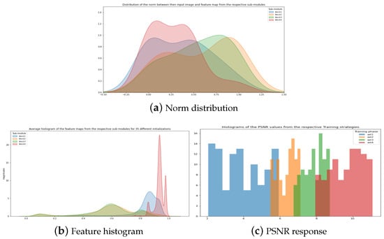
Figure 8.
(a) Distribution of norm between the feature map response and the input image. (b) Average histogram of the feature maps from the sub-modules. (c) PSNR distribution for different training setup.
Similarly, in Figure 8b, we show the average histogram of the feature map. As expected, each module shows a different histogram in comparison to the other. More explicitly, blocks 2 and 3 show a nearly similar distribution in each figure because both are the same block except for the number of channels associated with them. Another thing worth noting is that the histogram form the module 2 and 3 is covering the whole range between 0 and 1. This behavior justifies the reconstruction efficacy of the U-Net family networks. On the other hand, blocks 1 and 4 show the histogram information around 0.7 to 1. This particular trait indicates that these blocks capture the haze information since hazy pixels tend to higher in value.
In Figure 8c, we showed another graph to justify our overall network structure’s efficacy. We selected 20 images randomly and create a small dataset out using data augmentation. Then, we designed our different training strategy to do the following experiment. In the experiment, we train our original network with the small dataset mentioned above. We call this set 4. For set 3, we randomly selected only three blocks out of 4 and train the network with the same dataset again. This strategy is set 3 as in Figure 8c. Similarly, we randomly select two blocks and one block only out of 4 original blocks and label their training instances set 2 and set 1. Later, we perform the validation for those trained networks, and their PSNR result is present in Figure 8c. Clearly, our original network (set 4) shows better performance with this tiny dataset compared to its sub-modules alone.
However, our method is still not ideal in terms of performance. For example, we have not yet solved the challenges within the extreme hazy dataset. In our future work, we would like to redesign our training set to solve this task. We hope to work with more complex haze scenarios to achieve better performance in the extreme dehazing dataset. We would also like to improve the network’s performance by instance-learning. By doing so, we can improve the overall adaptivity of the proposed network. Furthermore, we would like to extend our work for object and face detection for the given hazy image.
5. Conclusions
This study proposes an end-to-end image dehazing method to recover the clean image from the given input. In our scheme, we introduced several improvements over the usual deep learning architectures. We also improve the performance of the typical L1 loss function for low-level computer vision tasks. Our study covers the image dehazing performance over several datasets. For each dataset, our dehazing network has achieved better performance in contrast to the compared studies. Additionally, we provide the necessary evidence to show that our sub-networks can capture different information to recover the hazy image. In future work, we plan to extend our current method for real-time video and detection tasks.
Author Contributions
Conceptualization, M.A.-N.I.F.; Formal analysis, M.A.-N.I.F.; Funding acquisition, H.Y.J.; Investigation, M.A.-N.I.F.; Methodology, M.A.-N.I.F.; Project administration, H.Y.J.; Resources, H.Y.J.; Supervision, H.Y.J.; Validation, M.A.-N.I.F.; Writing—original draft, M.A.-N.I.F.; Writing—review & editing, H.Y.J. The authors have contributed equally. All authors have read and agreed to the published version of the manuscript.
Funding
This work was supported by the National Research Foundation of Korea (NRF) grant funded by the Korea government (MSIT) (No. NRF-2021R1A2C1009776), and in part by the Research Fund of Chosun University 2020.
Conflicts of Interest
The authors declare no conflict of interest.
References
- Koschmieder, H. Theorie der Horizontalen Sichtweite: Kontrast und Sichtweite; Keim & Nemnich Press: Munich, Germany, 1925; pp. 25–33. [Google Scholar]
- Li, B.; Ren, W.; Fu, D.; Tao, D.; Feng, D.; Zeng, W.; Wang, Z. Reside: A benchmark for single image dehazing. arXiv 2017, arXiv:1712.04143. [Google Scholar]
- Ancuti, C.; Ancuti, C.O.; De Vleeschouwer, C.; Bovik, A.C. Night-time dehazing by fusion. In Proceedings of the IEEE International Conference on Image Processing (ICIP), Phoenix, AZ, USA, 25–28 September 2016; pp. 2256–2260. [Google Scholar]
- Ancuti, C.O.; Ancuti, C.; Hermans, C.; Bekaert, P. A fast semi-inverse approach to detect and remove the haze from a single image. In Proceedings of the Asian Conference on Computer Vision, Queenstown, New Zealand, 8–12 November 2010; Springer: Berlin/Heidelberg, Germany, 2010; pp. 501–514. [Google Scholar]
- Emberton, S.; Chittka, L.; Cavallaro, A. Hierarchical rank-based veiling light estimation for underwater dehazing. In Proceedings of the British Machine Vision Conference (BMVC), Swansea, UK, 7–10 September 2015; Xie, X., Jones, M.W., Tam, G.K.L., Eds.; BMVA Press: Surrey, UK, 2015; pp. 125.1–125.12. [Google Scholar]
- He, K.; Sun, J.; Tang, X. Single image haze removal using dark channel prior. IEEE Trans. Pattern Anal. Mach. Intell. 2011, 33, 2341–2353. [Google Scholar] [PubMed]
- Meng, G.; Wang, Y.; Duan, J.; Xiang, S.; Pan, C. Efficient image dehazing with boundary constraint and contextual regularization. In Proceedings of the IEEE International Conference on Computer Vision (ICCV), Sydney, Australia, 1–8 December 2013; pp. 617–624. [Google Scholar]
- Tarel, J.P.; Hautiere, N. Fast visibility restoration from a single color or gray level image. In Proceedings of the IEEE International Conference on Computer Vision, Kyoto, Japan, 27 September–4 October 2009; pp. 2201–2208. [Google Scholar]
- Cai, B.; Xu, X.; Jia, K.; Qing, C.; Tao, D. Dehazenet: An end-to-end system for single image haze removal. IEEE Trans. Image Process. 2016, 25, 5187–5198. [Google Scholar] [CrossRef] [PubMed]
- Ren, W.; Liu, S.; Zhang, H.; Pan, J.; Cao, X.; Yang, M.H. Single image dehazing via multi-scale convolutional neural networks. In Proceedings of the European Conference on Computer Vision, Amsterdam, The Netherlands, 8–16 October 2016; Springer: Cham, Switzerland, 2016; pp. 154–169. [Google Scholar]
- Swami, K.; Das, S.K. CANDY: Conditional adversarial networks based fully end-to-end system for single image haze removal. arXiv 2018, arXiv:1801.02892. [Google Scholar]
- Yang, X.; Xu, Z.; Luo, J. Towards perceptual image dehazing by physics-based disentanglement and adversarial training. In Proceedings of the Thirty-Second AAAI Conference on Artificial Intelligence (AAAI-18), New Orleans, LA, USA, 2–7 February 2018. [Google Scholar]
- Zhang, H.; Sindagi, V.; Patel, V.M. Joint transmission map estimation and dehazing using deep networks. arXiv 2017, arXiv:1708.00581. [Google Scholar] [CrossRef]
- Zhu, Q.; Mai, J.; Shao, L. A fast single image haze removal algorithm using color attenuation prior. IEEE Trans. Image Process. 2015, 24, 3522–3533. [Google Scholar]
- Berman, D.; Avidan, S. Non-local image dehazing. In Proceedings of the IEEE Conference on Computer Vision and Pattern Recognition (CVPR), Las Vegas, NV, USA, 27–30 June 2016; pp. 1674–1682. [Google Scholar]
- Berman, D.; Treibitz, T.; Avidan, S. Air-light estimation using haze-lines. In Proceedings of the IEEE International Conference on Computational Photography (ICCP), Stanford, CA, USA, 12–14 May 2017; pp. 1–9. [Google Scholar]
- Cozman, F.; Krotkov, E. Depth from scattering. In Proceedings of the IEEE Computer Society Conference on Computer Vision and Pattern Recognition, San Juan, PR, USA, 17–19 June 1997. [Google Scholar]
- Nayar, S.K.; Narasimhan, S.G. Vision in bad weather. In Proceedings of the Seventh IEEE International Conference on Computer Vision, Kerkyra, Greece, 20–27 September 1999. [Google Scholar]
- Nayar, S.K.; Narasimhan, S.G. Vision and the atmosphere. Int. J. Comput. Vis. 2002, 48, 233–254. [Google Scholar]
- Oakley, J.P.; Bu, H. Correction of simple contrast loss in color images. IEEE Trans. Image Process. 2007, 16, 511–522. [Google Scholar] [CrossRef] [PubMed]
- Fattal, R.; Agarwala, M.; Ruskinkiewicz, S. Multiscale shape and detail enhancement from multi-light image collections. ACM Trans. Graph. 2007, 26, 51. [Google Scholar] [CrossRef]
- Tan, R.T. Visibility in bad weather from a single image. In Proceedings of the IEEE CVPR, Anchorage, AK, USA, 24–26 June 2008. [Google Scholar]
- Chavez, P.S. An improved dark-object subtraction technique for atmonspheric scattering correction of multispectral data. Remote Sens. Environ. 2008, 82, 450–479. [Google Scholar]
- Zhang, Y.; Guindon, B.; Cihlar, J. An image transform to characterize and compensate for spatial variations in thin cloud contamination of landsat images. Remote Sens. Environ. 2002, 82, 173–187. [Google Scholar] [CrossRef]
- Du, Y.; Guindon, B.; Cihlar, J. Haze detection and removal in high resolution satellite image with wavelet analysis. IEEE Trans. Geosci. Remote Sens. 2002, 40, 210–217. [Google Scholar]
- Larson, G.W.; Rushmeier, H.; Piatko, C. A visibility matching tone reproduction operator for high dynamic range scenes. IEEE Trans. Vis. Comput. Graph. 1997, 3, 291–306. [Google Scholar] [CrossRef]
- Rahman, Z.; Jobson, D.; Woodwell, G. Multiscale retinex for color image enhancement. In Proceedings of the 3rd IEEE International Conference on Image Processing, Lausanne, Switzerland, 19 September 1996. [Google Scholar]
- Lu, J.; Healy, D.M. Contrast enhancement via multiscale gradient transformation. In Proceedings of the IEEE International Conference on Image Processing, Austin, TX, USA, 13–16 November 1994; pp. 482–486. [Google Scholar]
- Fattal, R. Image upsampling via imposed edge statistics. In Proceedings of the ACM SIGGRAPH, San Diego, CA, USA, 5–9 August 2007. [Google Scholar]
- Li, B.; Peng, X.; Wang, Z.; Xu, J.; Feng, D. AOD-Net: All-in-One Dehazing Network. In Proceedings of the IEEE International Conference on Computer Vision (ICCV), Venice, Italy, 22–29 October 2017; pp. 4770–4778. [Google Scholar] [CrossRef]
- Mei, K.; Jiang, A.; Li, J.; Wang, M. Progressive Feature Fusion Network for Realistic Image Dehazing. In Proceedings of the Asian Conference on Computer Vision, Perth, WA, Australia, 2–6 December 2018; pp. 203–215. [Google Scholar] [CrossRef]
- Rawat, W.; Wang, Z. Deep Convolutional Neural Networks for Image Classification: A Comprehensive Review. Neural Comput. 2017, 29, 2352–2449. [Google Scholar] [CrossRef] [PubMed]
- Zheng, C.; Fan, X.; Wang, C.; Qi, J. GMAN: A Graph Multi-Attention Network for Traffic Prediction. In Proceedings of the AAAI Conference on Artificial Intelligence, New York, NY, USA, 7–12 February 2020. [Google Scholar]
- Engin, D.; Genc, A.; Ekenel, H. Cycle-Dehaze: Enhanced CycleGAN for Single Image Dehazing. In Proceedings of the 2018 IEEE Conference on Computer Vision and Pattern Recognition Workshops, Salt Lake City, UT, USA, 18–22 June 2018; pp. 938–9388. [Google Scholar] [CrossRef]
- Ulyanov, D.; Vedaldi, A.; Lempitsky, V. Deep Image Prior. Int. J. Comput. Vis. 2020, 128, 1867–1888. [Google Scholar] [CrossRef]
- Das, S.; Dutta, S. Fast Deep Multi-patch Hierarchical Network for Nonhomogeneous Image Dehazing. In Proceedings of the IEEE/CVF Conference on Computer Vision and Pattern Recognition (CVPR) Workshops, Seattle, WA, USA, 16–18 June 2020; pp. 1994–2001. [Google Scholar] [CrossRef]
- Zhang, K.; Zuo, W.; Zhang, L. FFDNet: Toward a Fast and Flexible Solution for CNN based Image Denoising. IEEE Trans. Image Process. 2018, 27, 4608–4622. [Google Scholar] [CrossRef]
- Zhu, J.-Y.; Park, T.; Isola, P.; Efros, A.A. Unpaired Image-to-Image Translation Using Cycle-Consistent Adversarial Networks. In Proceedings of the IEEE International Conference on Computer Vision (ICCV), Venice, Italy, 22–29 October 2017; pp. 2242–2251. [Google Scholar] [CrossRef]
- Engelmann, J.; Lessmann, S. Conditional Wasserstein GAN-based Oversampling of Tabular Data for Imbalanced Learning. Expert Syst. Appl. 2021, 114582. [Google Scholar] [CrossRef]
- Mirza, M.; Osindero, S. Conditional Generative Adversarial Nets. arXiv 2014, arXiv:1411.1784. [Google Scholar]
- Ding, X.; Wang, Y.; Xu, Z.; Welch, W.; Wang, Z. CcGAN: Continuous Conditional Generative Adversarial Networks for Image Generation. arXiv 2020, arXiv:2011.07466. [Google Scholar]
- Malav, R.; Kim, A.; Sahoo, S.; Pandey, G. DHSGAN: An End to End Dehazing Network for Fog and Smoke. In Proceedings of the Asian Conference on Computer Vision, Perth, WA, Australia, 2–6 December 2018. [Google Scholar] [CrossRef]
- Sulami, M.; Glatzer, I.; Fattal, R.; Werman, M. Automatic recovery of the atmo-spheric light in hazy images. In Proceedings of the IEEE International Conference on Computational Photography, Santa Clara, CA, USA, 2–4 May 2014. [Google Scholar]
- Agustsson, E.; Timofte, R. NTIRE 2017 Challenge on Single Image Super-Resolution: Dataset and Study. In Proceedings of the IEEE Conference on Computer Vision and Pattern Recognition (CVPR) Workshops, Honolulu, HI, USA, 22–25 May 2017; pp. 1122–1131. [Google Scholar] [CrossRef]
- Fahim, M.A.-N.I.; Jung, H.Y. Single Image Dehazing Using End-to-End Deep-Dehaze Network. In Proceedings of the SMA 2020, Jeju, Korea, 17–19 September 2020. [Google Scholar]
- Xiang, P.; Wang, L.; Wu, F.; Cheng, J.; Zhou, M. Single-image de-raining with feature-supervised generative adversarial network. IEEE Signal Process. Lett. 2019, 26, 650–654. [Google Scholar] [CrossRef]
- Lian, Q.; Yan, W.; Zhang, X.; Chen, S. Single image rain removal using image decomposition and a dense network. IEEE/CAA J. Autom. Sin. 2019, 6, 1428–1437. [Google Scholar] [CrossRef]
- Wang, W.; Yuan, X. Recent advances in image dehazing. IEEE/CAA J. Autom. Sin. 2017, 4, 410–436. [Google Scholar] [CrossRef]
Publisher’s Note: MDPI stays neutral with regard to jurisdictional claims in published maps and institutional affiliations. |
© 2021 by the authors. Licensee MDPI, Basel, Switzerland. This article is an open access article distributed under the terms and conditions of the Creative Commons Attribution (CC BY) license (https://creativecommons.org/licenses/by/4.0/).