Integrated Comfort-Adaptive Cruise and Semi-Active Suspension Control for an Autonomous Vehicle: An LPV Approach

Abstract

This paper presents an integrated linear parameter-varying (LPV) control approach of an autonomous vehicle with an objective to guarantee driving comfort, consisting of cruise and semi-active suspension control. First, the vehicle longitudinal and vertical dynamics (equipped with a semi-active suspension system) are presented and written into LPV state-space representations. The reference speed is calculated online from the estimated road type and the desired comfort level (characterized by the frequency weighted vertical acceleration defined in the ISO 2631 norm) using precomputed polynomial functions. Then, concerning cruise control, an LPV ${\mathcal{H}}_2$ controller using a linear matrix inequality (LMI) based polytopic approach combined with the compensation of the estimated disturbance forces is developed to track the comfort-oriented reference speed. To further enhance passengers’ comfort, a decentralized LPV ${\mathcal{H}}_2$ controller for the semi-active suspension system is proposed, minimizing the effect of the road profile variations. The interaction with cruise control is achieved by the vehicle’s actual speed being a scheduling parameter for suspension control. To assess the strategy’s performance, simulations are conducted using a realistic nonlinear vehicle model validated from experimental data. The simulation results demonstrate the proposed approach’s capability to improve driving comfort.

1. Introduction

Autonomous vehicles always remain an interesting research topic thanks to their numerous advantages, including collision avoidance and fuel consumption reduction capabilities, satisfying traffic safety and environmental objectives.

There has been a considerable amount of research work conducted on either cruise or suspension control of autonomous vehicles. Cruise control refers to the control of the vehicle speed, which is related to longitudinal dynamics, for multiple purposes such as collision avoidance [1,2]. For this, different control strategies (optimal, robust, linear parameter-varying (LPV), etc.) have been proposed [3,4,5,6,7]. Recently, cruise control has been linked to a comfort objective [8,9,10], which extends the field to the coordination between longitudinal and vertical controllers.

Indeed, the suspension system is a key subsystem that allows us to improve the driving comfort and road-holding performance of the vehicle [11,12]. This is thanks to its remarkable ability to limit the vertical oscillations of the vehicle body caused by road displacements at the four wheels. From recent years, it is known that the semi-active suspension system provides better performance than the passive one while being less energy-consuming than the active one [12]. Existing work on semi-active suspension control includes model predictive control or state feedback with various observers, from robust, LPV, to unified ones [11,12,13,14,15].

However, there has not been much work combining cruise and suspension control into an integrated problem, considering their interaction. Besides, very few studies do consider the driving comfort level in a cruise control problem. To improve driving comfort, a potential strategy is to relate the speeds at which the vehicle should travel to the desired comfort level and w.r.t specific road profiles. Such speed values are determined using criteria formed by examining the human body, including which range of frequency is most absorbed by humans. Our group has conducted a study [16] into relating the vehicle speed with the comfort level measured using the ISO 2631 standard [17] and the international roughness index (IRI) [18] for each road type from A to D (defined in [19]). Recent research about road profile estimation using adaptive observers allows us to detect which road type the vehicle is traveling on [20], thus enabling this strategy.

The purpose of this paper is to bring further results and to introduce a comfort-oriented strategy of the integrated cruise–suspension control of an autonomous vehicle. There has been some existing work combining these problems [9,21]. In the latter, the coupling between longitudinal and vertical motions is considered but not the comfort objective. The work [9] requires too many assumptions and much information from the environment (therefore being challenging to embed in reality). Therefore, this work proposes a more realistic approach, handling unknown inputs using a robust LPV control approach. We analyze both longitudinal and vertical dynamics and their interaction through the road displacement at each of the four wheels. The ${\mathcal{H}}_2$ condition is used as it is suited for the type of noise we are faced with in this suspension control case where one of the sensors is an accelerometer. For cases where the variation of a specific parameter(s) significantly affects the system, we model the parameter(s) into an LPV problem, which is solved as a set of linear matrix inequalities (LMIs). We also show how driving comfort is evaluated by measuring the vertical acceleration transmitted to passengers, from which we propose a way to relate the current speed to comfort level using the ISO 2631 standard. This allows us to determine which speed the vehicle should travel at in order to guarantee that the acceleration felt by one passenger does not exceed a predefined value. Combining the cruise and suspension controllers with a comfort-oriented reference speed generation algorithm leads to the proposed integrated comfort-oriented vehicle control. The integrated control scheme is then tested using simulations on a realistic nonlinear vehicle model validated from experimental data.

This paper is organized as follows. In Section 2, we present the vehicle longitudinal and vertical dynamics (quarter-car model) then the integrated dynamics model. The general scheme of the strategy is presented in Section 3, which consists of comfort-guaranteeing speed calculation (described in detail in Section 4) and integrated cruise–suspension control (discussed in Section 5). Finally, simulation results are presented in Section 6, which shows the effectiveness of our strategy.

2. Vehicle Dynamics Modeling

This section introduces and discusses the vehicle longitudinal and vertical dynamics considered in this paper. The integrated full-vehicle model is also briefly presented.

2.1. Longitudinal Dynamics

In this part, we present the vehicle longitudinal dynamics and the corresponding system’s LPV state-space representation. First, let us make some assumptions for the longitudinal dynamics system:

• The vehicle mass is considered to be time-varying. It is measured online thanks to multiple built-in sensors that detect the additional load (the mass of the empty vehicle is the known nominal mass). This is the most crucial assumption as it allows for gain-scheduling based on mass. The vehicle speed is also directly measurable using a speedometer;
• The road slope is known/estimated in real time thanks to algorithms such as in [22,23,24]. Such an assumption allows us to implement road slope compensation using a feed-forward term in the cruise control input.

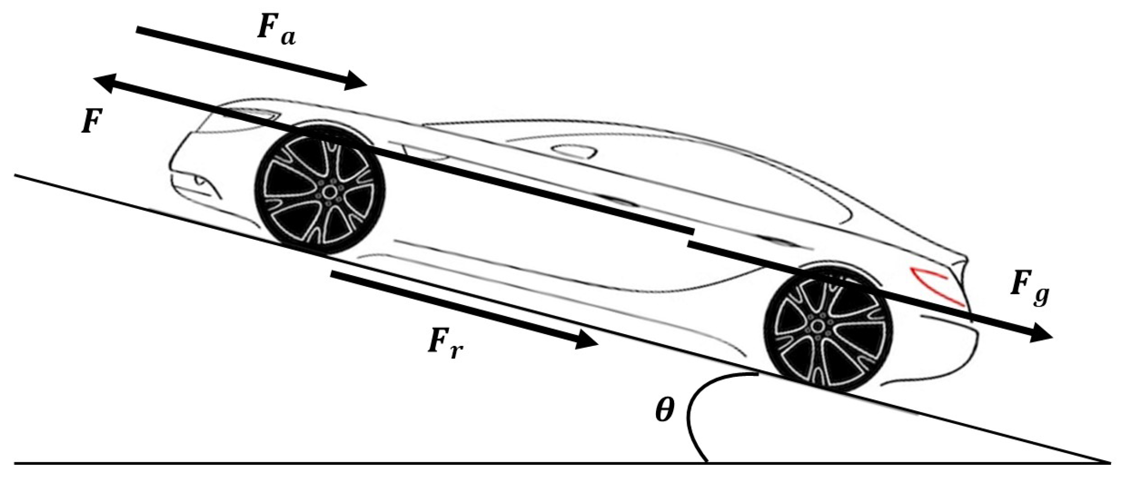
Suppose we have a vehicle of mass m traveling at the speed of v, as shown in Figure 1. Let F be the longitudinal control force on the vehicle, and $F_d$ the total disturbance force.

We have the following equation of motion [3]:

$$m\dot{v}=F-F_d.$$

(1)

The disturbance force $F_d$ consists of three components: The rolling friction supposed to have a constant value, the drag by gravity supposing the road slope $\theta$ to be sufficiently small (between $\pm {10}^{\circ }$ which is a realistic assumption for real roads), and the aerodynamic drag that adds nonlinearity to the system, respectively:

$$F_r=mg{C}_{r}cos\left(\theta \right)\approx mg{C}_r,$$

(2)

$$F_g=mgsin\left(\theta \right)\approx mg\theta ,$$

(3)

$$F_a=\frac{1}{2}{C}_v{D}_{a}S{v}^2,$$

(4)

where $C_r$ is the rolling friction coefficient, $C_v$ is the aerodynamic drag coefficient, $D_a$ is the air’s density, and S denotes the vehicle’s frontal area. The disturbance force thus has the following equation:

$$F_d=mg{C}_r+mg\theta +\frac{1}{2}{C}_v{D}_{a}S{v}^2.$$

(5)

Finally, the vehicle’s motion equation is formulated as:

$$m\dot{v}=F-mg{C}_r-mg\theta -\frac{1}{2}{C}_v{D}_{a}S{v}^2.$$

(6)

The input force F is composed of two parts:

$$F=F_{ff}+F_l,$$

(7)

where $F_{ff}=mg{\widehat{C}}_r+mg\widehat{\theta }$ is the feed-forward term that compensates for the rolling friction and the road slope and $F_l$ is the feedback term of the longitudinal control force. Here ${\widehat{C}}_r$ is an estimated nominal value for $C_r$ (constant) and $\widehat{\theta }$ is the road slope estimated in real time by the methods in [22,23,24]. As this compensation is inexact, i.e., ${\widehat{C}}_r\ne C_r$ and $\widehat{\theta }\ne \theta$, all the uncertainty is modeled by $\Delta w_l$, where $\Delta$ is a constant bound and $w_l$ is white noise ($|w_l|\le 1$).

The system is then written in the LPV form, with $x_l=v$ being the state variable, $u_l=F_l$ being the cruise control input, $y_l=v$ being the measured output, and ${\rho }_l={\left[\begin{array}{cc}{\rho }_{l1}& {\rho }_{l2}\end{array}\right]}^{\top }={\left[\begin{array}{cc}1/m& v\end{array}\right]}^{\top }$ being the varying parameter of the longitudinal control case, as:

$${\Sigma }_l\left({\rho }_l\right):\left\{\begin{array}{c}{\dot{x}}_l=A_l\left({\rho }_l\right)x_l+B_{l1}{w}_l+B_{l2}\left({\rho }_l\right)u_l\hfill \\ y_l=C_l{x}_l+D_{l1}{w}_l+D_{l2}{u}_l,\hfill \end{array}\right.$$

(8)

where:

$$A_l\left({\rho }_l\right)=\left[-\frac{1}{2}{C}_v{D}_{a}S{\rho }_{l1}{\rho }_{l2}\right],B_{l1}=[-g\Delta ],B_{l2}\left({\rho }_l\right)=\left[{\rho }_{l1}\right],C_l=\left[1\right],D_{l1}=\left[0\right],D_{l2}=\left[0\right].$$

Vehicle longitudinal dynamics parameters are given in

Table 1. Longitudinal dynamics parameters.

Symbol	Value	SI Unit	Parameter Name
m	1400	kg	Vehicle mass
$C_r$	0.01	-	Rolling friction coefficient
$C_v$	0.32	-	Aerodynamic drag coefficient
$D_a$	1.3	kg/m${}^3$	Density of air
S	2.4	m${}^2$	Vehicle frontal area
g	9.8	m/s${}^2$	Gravitational acceleration
$\tau$	0.1	s	Actuator time constant
$\sigma$	0.2	s	Communication delay in the vehicle
$v_{wind}$	12	km/h	Average wind speed

.

2.2. Vertical Dynamics

The suspension control design is carried out using the quarter-car suspension system [11]. Indeed, this model is simple enough to catch the comfort objective w.r.t the bounce motion and to cope with the requirements about reducing the complexity of an embedded controller. For pitch/roll control, a full-vehicle model would be needed, which is not the case here.

We use the quarter-car model with a semi-active magneto-rheological (MR) suspension system to model the vehicle vertical dynamics, as shown in Figure 2. This consists of the sprung mass $m_s$, the unsprung mass $m_{us}$, and the suspension components positioned between them, including a spring element with stiffness $k_s$ and the damper part. Let us denote $z_s$ and $z_{us}$ as the sprung and unsprung mass’ displacement, respectively.

From Newton’s second law of motion, we obtain:

$$\left\{\begin{array}{c}{m}_s{\ddot{z}}_s=-F_{spring}-F_{damper}\hfill \\ m_{us}{\ddot{z}}_{us}=F_{spring}+F_{damper}-F_{tire},\hfill \end{array}\right.$$

(9)

where $F_{spring}=k_s(z_s-z_{us})$ is the spring force and $F_{tire}=k_t(z_{us}-z_r)$ is the tire force.

Concerning the damper force $F_{damper}$, two models are considered:

• A control-oriented model as given below:

  $$F_{damper}=\underset{F_{passive}}{\underbrace{k_0(z_s-z_{us})+c_0({\dot{z}}_s-{\dot{z}}_{us})}}+F_v,$$

  (10)

  where $F_v$ is the control input;
• A simulation model as given below and shown in Figure 3:

  $$F_{damper}=k_0(z_s-z_{us})+c_0({\dot{z}}_s-{\dot{z}}_{us})+I·f_c·tanh(k_1(z_s-z_{us})+c_1({\dot{z}}_s-{\dot{z}}_{us})),$$

  (11)

  where $c_0$, $k_0$, $c_1$, and $k_1$ are constant parameters and I is the applied current. In order to design the controller, the controlled part in (11) is defined as $F_v=I·f_c·tanh(k_1(z_s-z_{us})+c_1({\dot{z}}_s-{\dot{z}}_{us}))$.

In Figure 3, the considered MR damper force – deflection velocity (${\dot{z}}_{def}={\dot{z}}_s-{\dot{z}}_{us}$) characteristic is shown, from the MR damper available at ITESM, Mexico (refer to [25]).

The model in (10) is used to design the controller. Then, the nonlinear model (11) is used as the inverse model to simulate the suspension controlled system for the full car model presented later.

Remark 1: The controller to be designed in this paper is applied to the semi-active suspension system using the clipped strategy as used in [26]. Then, the control input current to be applied to the MR damper is computed from the clipped controlled damper force and given the deflection ($z_{def}=z_s-z_{us}$) and the deflection velocity ${\dot{z}}_{def}$.

To link with longitudinal dynamics, we here consider benefiting from some knowledge of the road displacement input model $z_r$, which is related to the current vehicle speed according to [27] as:

$${\dot{z}}_r+a·v·z_r=b·v·w_v,$$

(12)

where $w_v$ is white noise, and a and b are coefficients that depend on the road type according to International Organization for Standardization (ISO) classification [19].

Remark 2: Using a road profile model is indeed possible since the information on the type of road profile may be obtained using some adaptive road profile estimator, as proposed in [20], or a frequency-wise approach [27].

From (9) and (12), by selecting the system states as $x_v={\left[\begin{array}{ccccc}{z}_s& {\dot{z}}_s& z_{us}& {\dot{z}}_{us}& z_r\end{array}\right]}^{\top }\in {\mathbb{R}}^5$, the measured variables $y_v={\left[\begin{array}{cc}{\ddot{z}}_s& z_s-z_{us}\end{array}\right]}^{\top }\in {\mathbb{R}}^2$, the control input $u_v=F_v$, and by choosing the scheduling variable ${\rho }_v=v$ to link with longitudinal dynamics, the extended quarter-car system can be written in the LPV form as:

$${\Sigma }_v\left({\rho }_v\right):\left\{\begin{array}{c}{\dot{x}}_v=A_v\left({\rho }_v\right)x_v+B_{v1}\left({\rho }_v\right)w_v+B_{v2}{u}_v\hfill \\ y_v=C_{v2}{x}_v+D_{v21}{w}_v+D_{v22}{u}_v,\hfill \end{array}\right.$$

(13)

where:

$$\begin{array}{c}{A}_v\left({\rho }_v\right)=\left[\begin{array}{ccccc}0& 1& 0& 0& 0\\ -\frac{k}{m_s}& -\frac{c_0}{m_s}& \frac{k}{m_s}& \frac{c_0}{m_s}& 0\\ 0& 0& 0& 1& 0\\ \frac{k}{m_{us}}& \frac{c_0}{m_{us}}& -\frac{k+k_t}{m_{us}}& -\frac{c_0}{m_{us}}& \frac{k_t}{m_{us}}\\ 0& 0& 0& 0& -a·{\rho }_v\end{array}\right],B_{v1}\left({\rho }_v\right)=\left[\begin{array}{c}0\\ 0\\ 0\\ 0\\ b·{\rho }_v\end{array}\right],B_{v2}=\left[\begin{array}{c}0\\ -\frac{1}{m_s}\\ 0\\ \frac{1}{m_{us}}\\ 0\end{array}\right],\hfill \\ C_{v2}=\left[\begin{array}{ccccc}-\frac{k}{m_s}& -\frac{c_0}{m_s}& \frac{k}{m_s}& \frac{c_0}{m_s}& 0\\ 1& 0& -1& 0& 0\end{array}\right],D_{v21}=\left[\begin{array}{c}0\\ 0\end{array}\right],D_{v22}=\left[\begin{array}{c}-\frac{1}{m_s}\\ 0\end{array}\right],\hfill \end{array}$$

where $k=k_s+k_0$. In this work, the coefficients a and b are consistent with those of a road profile of type B in [19].

Vehicle vertical dynamics parameters are given in

Table 2. Vertical dynamics parameters.

Symbol	Value	SI Unit	Parameter Name
$m_s$	315	kg	Sprung mass
$m_{us}$	37.5	kg	Unsprung mass
$c_0$	3000	Ns/m	Viscous damping coefficient
$k=k_s+k_0$	29,500	N/m	Spring and damper stiffness
$k_t$	208,000	N/m	Tire stiffness

.

2.3. Full-Vehicle Dynamics

In this paper, the full-vehicle model presented in [28,29] is used for simulation and validation purposes. This model and its parameters have been validated on a real Renault Megane vehicle (thanks to M. Basset, from the MIAM research team). For illustration, the model is presented in Figure 4, but interested readers should refer to [28] for more details.

Note that the main interest in using the full nonlinear vehicle model is that it allows us to consider a nonlinear load transfer, fast nonlinear dynamics entering the tire force description, and consequently, in the global chassis dynamic. It reproduces the longitudinal (x), lateral (y), vertical (z), roll ($\theta$), pitch ($\varphi$), and yaw ($\psi$) dynamics of the chassis. It also models the vertical and rotational motions of the wheels ($z_{{us}_{ij}}$ and ${\omega }_{ij}$ respectively), the slip ratios (${\lambda }_{ij}$), and the center of gravity side slip angle (${\beta }_{cog}$) dynamics, as a function of the tires and suspensions forces.

3. Integrated Cruise—Suspension LPV Control of an Autonomous Vehicle for Comfort: Structure and Objectives

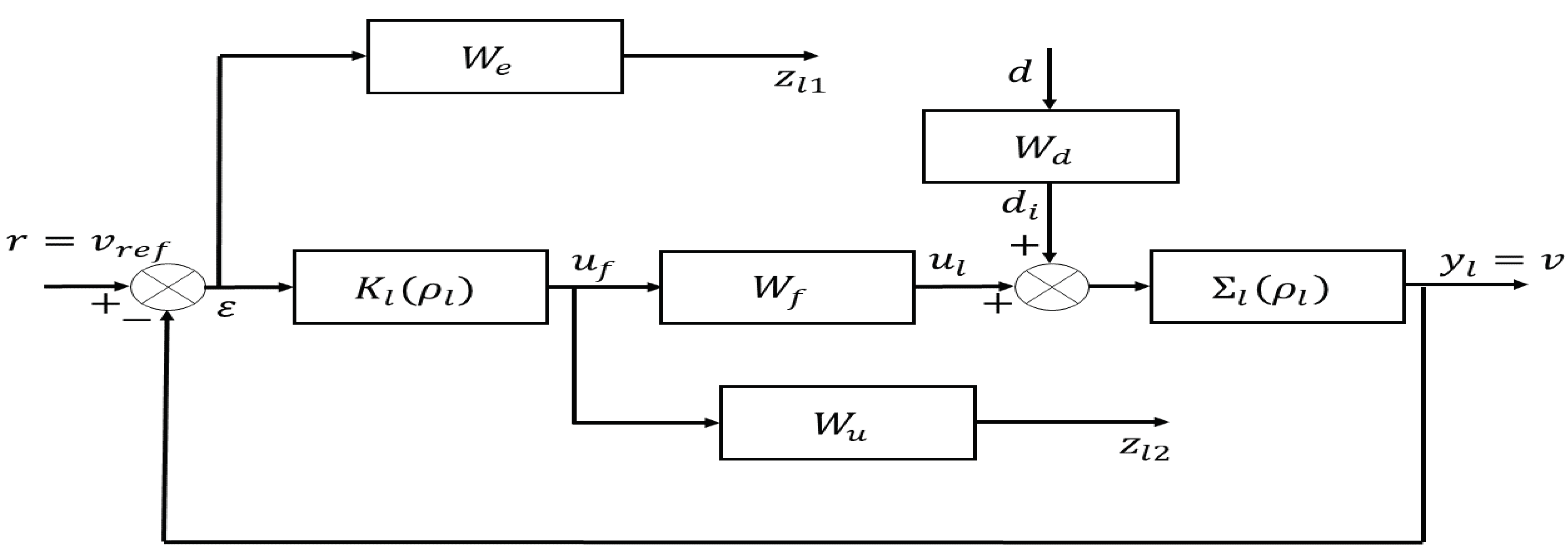
The proposed strategy is illustrated in Figure 5.

Our strategy consists of three main parts closely connected to each other and the full-vehicle dynamics. Note that the vehicle speed connects the longitudinal and vertical dynamics due to the relationship (12).

The road type is assumed to be known/estimated in real time thanks to algorithms such as in [20]. This is the condition that enables the making of the proposed reference speed generation strategy, which gives us suitable speed values based on the road profile and comfort objective. In the reference speed calculation part, given the estimated road type and the desired comfort level specified by the driver/passenger(s), a suitable reference speed value is determined so as to guarantee this level. How we quantify driving comfort and calculate the reference speed is presented in Section 4.

In the cruise control part, given the calculated reference speed value, the cruise controller drives the vehicle speed to track this value. This uses not only the feedback measured by the speedometer but also road information such as road slope in order to compensate for this, providing a smoother response. How we design this part is discussed in Section 5.2.

In the semi-active suspension control design method, a semi-active suspension control strategy is used to further improve driving comfort. How we design this part is discussed in Section 5.3.

Combining the three mentioned parts constitutes what we propose in this paper as the integrated cruise–suspension control of an autonomous vehicle with a comfort objective.

4. Comfort-Oriented Reference Speed Calculation

4.1. Comfort Evaluation Using the ISO 2631 Standard

First, the road types are characterized by the ISO norm [19]. In Figure 6, we examine the road displacement profiles of types from A to D described in the ISO standard, with the vehicle’s speed being 15 m/s. As shown in [30], such profiles do change w.r.t the speed as we considered in the modeling step (see (12)).

This displacement is then transmitted to the passengers through the vehicle vertical dynamics. What affects driving comfort is the acceleration felt by passengers, as analyzed in the ISO 2631 norm [17]. In order to characterize human comfort, i.e., the effect of exposure to vibration, a filter is applied on the sprung mass acceleration [31]. This filter’s transfer function is:

$$W_{ISO}\left(s\right)=\frac{81.89s^3+796.6s^2+1937s+0.1446}{s^4+80s^3+2264s^2+7172s+21196}.$$

(14)

Driving comfort is then assessed according to the following scale of the ISO 2631 standard using the root mean square (RMS) value of the vertical acceleration [17] (see

Table 3. Vertical acceleration RMS (root mean square) value and comfort level.

RMS Value of Acceleration	Comfort Level
Less than 0.315 m/s${}^2$	Not uncomfortable
0.315–0.63 m/s${}^2$	A little uncomfortable
0.5–1 m/s${}^2$	Fairly uncomfortable
0.8–1.6 m/s${}^2$	Uncomfortable
1.25–2.5 m/s${}^2$	Very uncomfortable
Greater than 2 m/s${}^2$	Extremely uncomfortable

).

4.2. Modeling of Vehicle Speed—Comfort Interaction

It is known that, as the vehicle travels on certain different road types with the same speed and vice versa, it experiences different road displacement profiles. Thus, the felt human comfort varies according to the vehicle speed [30,32].

Our objective is to propose a comfort-oriented reference speed profile to link the comfort level to the vehicle’s speed. This is carried out using a vertical vehicle model performing simulation with different speed values and computing the comfort criterion. This allows us first to evaluate the human comfort (for the RMS of the vertical acceleration) as seen in Figure 7.

Then, following our previous study in [16], we define the comfort-oriented reference speed values from a polynomial fitting method, which are illustrated in Figure 8 and

Table 4. Calculation of comfort-oriented reference speed values.

Road Type	Comfort-Oriented Reference Speed Values ${\mathit{v}}_{\mathbf{ref}}\left(\mathit{x}\right)$ Where x is RMS Acceleration
A	$-281058.82x^7+616932.65x^6-553287.74x^5+259269.77x^4-67006.34x^3$ $+9126.1x^2-490.82x+17.03$
B	$-2918.46x^7+12566.60x^6-22133.93x^5+20420.08x^4-10438.88x^3$ $+2839.03x^2-319.40x+20.36$
C	$-20.58x^7+176.82x^6-620.95x^5+1140.85x^4-1158.9x^3$ $+623.06x^2-134.38x+17.84$
D	$-0.19x^7+3.22x^6-22.33x^5+81.06x^4-162.92x^3$ $+174.09x^2-76.47x+19.57$

.

These polynomials are precomputed and programmed into the autonomous vehicle’s computer. In practice, the vehicle detects the current road type by performing the road estimation algorithm as assumed. Then from a given desired comfort level, characterized by a given RMS acceleration, the corresponding reference speed is calculated thanks to these polynomials.

5. LPV ${\mathcal{H}}_2$ Cruise and Semi-Active Suspension Control

In this section, both longitudinal and vertical controllers are synthesized using the ${\mathcal{H}}_2$ control approach for LPV systems. A short background of the control approach is presented herein, followed by the two design applications.

5.1. Preliminaries on LPV ${\mathcal{H}}_2$ Controller Design

Throughout this paper, we design two LPV controllers for cruise and semi-active suspension control. This part presents briefly the LPV approach including the optimization problem to be solved [28]. An LPV system is represented as:

$$\Sigma \left(\rho \right):\left[\begin{array}{c}\dot{x}\\ z\\ y\end{array}\right]=\left[\begin{array}{ccc}A\left(\rho \right)& B_1\left(\rho \right)& B_2\left(\rho \right)\\ C_1\left(\rho \right)& D_{11}\left(\rho \right)& D_{12}\left(\rho \right)\\ C_2\left(\rho \right)& D_{21}\left(\rho \right)& D_{22}\left(\rho \right)\end{array}\right]\left[\begin{array}{c}x\\ w\\ u\end{array}\right],$$

(15)

where x is the state, z is the controlled output, y is the measured output, w is the disturbance, u is the control input, and $\rho ={\left[\begin{array}{cccc}{\rho }_1& {\rho }_2& \dots & {\rho }_N\end{array}\right]}^{\top }\in \Omega$ is the vector of varying parameters ($\Omega$ is a convex set). The assumptions on $\rho$ are:

• $\rho$ varies in the set of continously differentiable parameter curves and is known or measurable;
• $\rho$ is bounded, i.e., ${\rho }_j\in [\underline{{\rho }_j},\overline{{\rho }_j}],\forall j$;
• The system matrices $A(·)$, etc. are continuous on $\Omega$.

The vector of parameters evolves inside a polytope represented by $2^N$ vertices ${\omega }_i$, as:

$$\rho \in \mathbf{Co}\{{\omega }_1,\dots ,{\omega }_Z\}.$$

(16)

It is then written as the convex combination:

$$\rho =\sum _{i=1}^{2^N}{\alpha }_i{\omega }_i,{\alpha }_i\ge 0,\sum _{i=1}^{2^N}{\alpha }_i=1,$$

(17)

where the vertices are defined by a vector ${\omega }_i=[{\nu }_{i1},\dots ,{\nu }_{iN}]$ where ${\nu }_{ij}$ equals $\underline{{\rho }_j}$ or $\overline{{\rho }_j}$.

Therefore, we consider a polytopic model of the LPV system above, represented as:

$$\Sigma \left(\rho \right)=\sum _{i=1}^{2^N}{\alpha }_i\left(\rho \right)\left[\begin{array}{cc}A\left({\omega }_i\right)& B\left({\omega }_i\right)\\ C\left({\omega }_i\right)& D\left({\omega }_i\right)\end{array}\right],{\alpha }_i\left(\rho \right)\ge 0,\sum _{i=1}^{2^N}{\alpha }_i\left(\rho \right)=1,$$

(18)

where $\left[\begin{array}{cc}A\left({\omega }_i\right)& B\left({\omega }_i\right)\\ C\left({\omega }_i\right)& D\left({\omega }_i\right)\end{array}\right]$ is the linear time-invariant (LTI) system corresponding to one of the system’s $2^N$ vertices.

An LPV controller has the following structure:

$$K\left(\rho \right):\left[\begin{array}{c}{\dot{x}}_c\\ u\end{array}\right]=\left[\begin{array}{cc}{A}_c\left(\rho \right)& B_c\left(\rho \right)\\ C_c\left(\rho \right)& D_c\left(\rho \right)\end{array}\right]\left[\begin{array}{c}{x}_c\\ y\end{array}\right].$$

(19)

Solving for an LPV controller using the ${\mathcal{H}}_2$ condition is here carried out using the polytopic approach so computing the controllers $K_i$$\forall i$, at each vertex of the parameter polytope, such that a single, global performance ${\gamma }_2$ is minimized. For a given parameter value $\rho$, the controller is then determined as:

$$K\left(\rho \right)=\sum _{i=1}^{2^N}{\alpha }_i\left(\rho \right)K_i,{\alpha }_i\left(\rho \right)\ge 0,\sum _{i=1}^{2^N}{\alpha }_i\left(\rho \right)=1.$$

(20)

Proposition 1.

A dynamical output-feedback controller $K\left(\rho \right)$ (19) that solves the control problem is obtained by solving the following LMIs in ($\mathit{X}\left(\rho \right)$, $\mathit{Y}\left(\rho \right)$, $\tilde{\mathit{A}}\left(\rho \right)$, $\tilde{\mathit{B}}\left(\rho \right)$, $\tilde{\mathit{C}}\left(\rho \right)$, and $\tilde{\mathit{D}}\left(\rho \right)$) at the $2^N$ vertices ${\omega }_i$ of the polytope, while minimizing ${\gamma }_2$:

$$\begin{array}{c}\left[\begin{array}{ccc}{M}_{11}& {(\ast )}^{\top }& {(\ast )}^{\top }\\ M_{21}& M_{22}& {(\ast )}^{\top }\\ M_{31}& M_{32}& M_{33}\end{array}\right]\prec 0,\forall i,\hfill \\ \left[\begin{array}{ccc}{N}_{11}& {(\ast )}^{\top }& {(\ast )}^{\top }\\ N_{21}& N_{22}& {(\ast )}^{\top }\\ N_{31}& N_{32}& N_{33}\end{array}\right]\succ 0,\forall i,\hfill \\ Trace\left(\mathit{Z}\right)<{\gamma }_2,\hfill \end{array}$$

(21)

where:

$$\begin{array}{ccc}\hfill M_{11}& =& A\left({\omega }_i\right)\mathit{X}\left({\omega }_i\right)+\mathit{X}\left({\omega }_i\right)A{\left({\omega }_i\right)}^{\top }+B_2\tilde{\mathit{C}}\left({\omega }_i\right)+\tilde{\mathit{C}}{\left({\omega }_i\right)}^{\top }{B}_2^{\top },\hfill \\ \hfill M_{21}& =& \tilde{\mathit{A}}\left({\omega }_i\right)+A{\left({\omega }_i\right)}^{\top }+C_2^{\top }\tilde{\mathit{D}}{\left({\omega }_i\right)}^{\top }{B}_2^{\top },\hfill \\ \hfill M_{22}& =& \mathit{Y}\left({\omega }_i\right)A\left({\omega }_i\right)+A{\left({\omega }_i\right)}^{\top }\mathit{Y}\left({\omega }_i\right)+\tilde{\mathit{B}}\left({\omega }_i\right)C_2+C_2^{\top }\tilde{\mathit{B}}{\left({\omega }_i\right)}^{\top },\hfill \\ \hfill M_{31}& =& B_1{\left({\omega }_i\right)}^{\top }+D_{21}{\left({\omega }_i\right)}^{\top }\tilde{\mathit{D}}{\left({\omega }_i\right)}^{\top }{B}_2^{\top },\hfill \\ \hfill M_{32}& =& B_1{\left({\omega }_i\right)}^{\top }\mathit{Y}\left({\omega }_i\right)+D_{21}{\left({\omega }_i\right)}^{\top }\tilde{\mathit{B}}{\left({\omega }_i\right)}^{\top },\hfill \\ \hfill M_{33}& =& -I_{n_u},\hfill \\ \hfill N_{11}& =& X\left({\omega }_i\right),\hfill \\ \hfill N_{21}& =& I_n,\hfill \\ \hfill N_{22}& =& Y\left({\omega }_i\right),\hfill \\ \hfill N_{31}& =& C_1\left({\omega }_i\right)\mathit{X}\left({\omega }_i\right)+D_{12}\left({\omega }_i\right)\tilde{\mathit{C}}\left({\omega }_i\right),\hfill \\ \hfill N_{32}& =& C_1\left({\omega }_i\right)+D_{12}\left({\omega }_i\right)\tilde{\mathit{D}}\left({\omega }_i\right)C_2,\hfill \\ \hfill N_{33}& =& \mathit{Z}.\hfill \end{array}$$

Then, the reconstruction of the controller $K_i$ is obtained by the following equivalent transformation:

$$\left\{\begin{array}{ccc}\hfill D_c\left({\omega }_i\right)& =& \tilde{\mathit{D}}\left({\omega }_i\right)\hfill \\ \hfill C_c\left({\omega }_i\right)& =& (\tilde{\mathit{C}}\left({\omega }_i\right)-D_c\left({\omega }_i\right)C_2\left({\omega }_i\right)\mathit{X}\left({\omega }_i\right))M{\left({\omega }_i\right)}^{-\top }\hfill \\ \hfill B_c\left({\omega }_i\right)& =& N{\left({\omega }_i\right)}^{-1}(\tilde{\mathit{B}}\left({\omega }_i\right)-\mathit{Y}\left({\omega }_i\right)B_2\left({\omega }_i\right)D_c\left({\omega }_i\right))\hfill \\ \hfill A_c\left({\omega }_i\right)& =& N{\left({\omega }_i\right)}^{-1}(\tilde{\mathit{A}}\left({\omega }_i\right)-\mathit{Y}\left({\omega }_i\right)A\left({\omega }_i\right)\mathit{X}\left({\omega }_i\right)-\mathit{Y}\left({\omega }_i\right)B_2\left({\omega }_i\right)D_c\left({\omega }_i\right)C_2\left({\omega }_i\right)\mathit{X}\left({\omega }_i\right)\hfill \\ \hfill & -& N\left({\omega }_i\right)B_c\left({\omega }_i\right)C_2\left({\omega }_i\right)\mathit{X}\left({\omega }_i\right)-\mathit{Y}\left({\omega }_i\right)B_2\left({\omega }_i\right)C_c\left({\omega }_i\right)M{\left({\omega }_i\right)}^{\top })M{\left({\omega }_i\right)}^{-\top },\hfill \end{array}\right.$$

(22)

where $M\left({\omega }_i\right)$ and $N\left({\omega }_i\right)$ are defined such that $M\left({\omega }_i\right)N{\left({\omega }_i\right)}^{\top }=I_n-X\left({\omega }_i\right)Y\left({\omega }_i\right)$ (that can be solved through a singular value decomposition plus a Cholesky factorization).

5.2. Application of the LPV ${\mathcal{H}}_2$ Approach to Cruise Control

5.2.1. Cruise Controller Design

The approach above is here applied to the LPV longitudinal model presented before in (8) as:

$${\Sigma }_l\left({\rho }_l\right):\left\{\begin{array}{c}{\dot{x}}_l=A_l\left({\rho }_l\right)x_l+B_{l1}{w}_l+B_{l2}\left({\rho }_l\right)u_l\hfill \\ y_l=C_l{x}_l+D_{l1}{w}_l+D_{l2}{u}_l,\hfill \end{array}\right.$$

(23)

where ${\rho }_l$ includes the vehicle mass and speed.

To use the polytopic approach, the control input matrix has to be independent of the scheduling parameter. Therefore, following the method in [33], the system is extended with the following filter at the input variable:

$$W_f:\left[\begin{array}{c}{\dot{x}}_f\\ u_l\end{array}\right]=\left[\begin{array}{cc}{A}_f& B_f\\ C_f& 0\end{array}\right]\left[\begin{array}{c}{x}_f\\ u_f\end{array}\right],$$

(24)

where $A_f$, $B_f$, and $C_f$ are constant matrices. Here, we choose $A_f=-1/{\tau }_f$, $B_f=1/{\tau }_f$, and $C_f=1$ where ${\tau }_f$ is a small constant. To synthesize the controller, we define the generalized system denoted ${\Sigma }_{gl}\left({\rho }_l\right)$ (see in Figure 9) consisting of the extended state-space representation with a parameter-independent control input:

$$\left\{\begin{array}{c}\left[\begin{array}{c}{\dot{x}}_l\\ {\dot{x}}_f\end{array}\right]=\left[\begin{array}{cc}{A}_l\left({\rho }_l\right)& B_{l2}\left({\rho }_l\right)C_f\\ 0& A_f\end{array}\right]\left[\begin{array}{c}{x}_l\\ x_f\end{array}\right]+\left[\begin{array}{c}{B}_{l1}\\ 0\end{array}\right]w_l+\left[\begin{array}{c}0\\ B_f\end{array}\right]u_f\hfill \\ y_l=\left[\begin{array}{cc}{C}_l& D_{l2}{C}_f\end{array}\right]\left[\begin{array}{c}{x}_l\\ x_f\end{array}\right]+D_{l1}{w}_l,\hfill \end{array}\right.$$

(25)

and the following weighting functions in order to ensure tracking performances and to cope with the actuator limitations:

$$\begin{array}{c}\hfill W_e=\frac{0.5s+2}{s+0.0002},W_u=\frac{1}{100},W_d=0.01.\end{array}$$

(26)

According to [33], since the parameter dependence is affine and since the scheduling parameter ${\rho }_l$ varies in a polytope of four vertices, i.e., ${\rho }_{l1}\in [\underline{{\rho }_{l1}},\overline{{\rho }_{l1}}]$ and ${\rho }_{l2}\in [\underline{{\rho }_{l2}},\overline{{\rho }_{l2}}]$, the generalized system ${\Sigma }_{gl}\left({\rho }_l\right)$ in Figure 9 can be expressed as a polytopic system composed of four vertices:

$$\begin{array}{c}\hfill {\Sigma }_{gl}\left({\rho }_l\right)=\sum _{i=1}^4{\alpha }_{l_i}\left({\rho }_l\right){\Sigma }_{{gl}_i},{\alpha }_{l_i}\left({\rho }_l\right)\ge 0,\sum _{i=1}^4{\alpha }_{l_i}\left({\rho }_l\right)=1,\end{array}$$

(27)

where ${\Sigma }_{{gl}_1}={\Sigma }_{gl}(\underline{{\rho }_{l1}},\underline{{\rho }_{l2}})$, ${\Sigma }_{{gl}_2}={\Sigma }_{gl}(\underline{{\rho }_{l1}},\overline{{\rho }_{l2}})$, ${\Sigma }_{{gl}_3}={\Sigma }_{gl}(\overline{{\rho }_{l1}},\underline{{\rho }_{l2}})$, and ${\Sigma }_{{gl}_4}={\Sigma }_{gl}(\overline{{\rho }_{l1}},\overline{{\rho }_{l2}})$. Solving the LMIs in Proposition 1, the LPV controller $K_l({\rho }_l)$ with the scheme as shown in Figure 9 is defined as:

$$K_l\left({\rho }_l\right):\left[\begin{array}{c}{\dot{x}}_{cl}\\ u_f\end{array}\right]=\left[\begin{array}{cc}{A}_{cl}\left({\rho }_l\right)& B_{cl}\left({\rho }_l\right)\\ C_{cl}\left({\rho }_l\right)& D_{cl}\left({\rho }_l\right)\end{array}\right]\left[\begin{array}{c}{x}_{cl}\\ ϵ\end{array}\right],$$

(28)

where $ϵ=r-y_l$ denotes the tracking error where r is the reference. The controller $K_l\left({\rho }_l\right)$ can be transformed into a convex interpolation as follows:

$$K_l\left({\rho }_l\right)=\sum _{i=1}^4{\alpha }_{l_i}\left({\rho }_l\right)\left[\begin{array}{cc}{A}_{{cl}_i}& B_{{cl}_i}\\ C_{{cl}_i}& D_{{cl}_i}\end{array}\right],{\alpha }_{l_i}\left({\rho }_l\right)\ge 0,\sum _{i=1}^4{\alpha }_{l_i}\left({\rho }_l\right)=1.$$

(29)

5.2.2. Cruise Control Simulation

We verify by simulation that the vehicle speed can track a given reference value in the presence of disturbance and noise in the form of inexact disturbance force compensation.

We see that the tracking performance is guaranteed, and tracking is achieved after a few hundreds of meters (see Figure 10), with a longitudinal control force smaller than 4000 N (see Figure 11).

5.3. Application of the LPV ${\mathcal{H}}_2$ Approach to Semi-Active Suspension Control

5.3.1. Semi-Active Suspension Controller Design

First, let us recall the LPV system where the extended quarter-car system is described in (13) as:

$${\Sigma }_v\left({\rho }_v\right):\left\{\begin{array}{c}{\dot{x}}_v=A_v\left({\rho }_v\right)x_v+B_{v1}\left({\rho }_v\right)w_v+B_{v2}{u}_v\hfill \\ y_v=C_{v2}{x}_v+D_{v21}{w}_v+D_{v22}{u}_v,\hfill \end{array}\right.$$

(30)

where ${\rho }_v$ is the vehicle speed.

In order to guarantee the comfort and road holding objectives, we define the performance output vector as $z_v={\left[\begin{array}{cc}{z}_{us}& {\ddot{z}}_s\end{array}\right]}^{\top }\in {\mathbb{R}}^2$. To synthesize the controller, we define the generalized system denoted ${\Sigma }_{gv}\left({\rho }_v\right)$ (see in Figure 12) consisting of:

$$\left\{\begin{array}{c}{\dot{x}}_v=A_v\left({\rho }_v\right)x_v+B_{v1}\left({\rho }_v\right)w_v+B_{v2}{u}_v\hfill \\ z_v=C_{v1}{x}_v+D_{v11}{w}_v+D_{v12}{u}_v\hfill \\ y_v=C_{v2}{x}_v+D_{v21}{w}_v+D_{v22}{u}_v,\hfill \end{array}\right.$$

(31)

where:

$$\begin{array}{c}{C}_{v1}=\left[\begin{array}{ccccc}0& 0& 1& 0& 0\\ -\frac{k}{m_s}& -\frac{c_0}{m_s}& \frac{k}{m_s}& \frac{c_0}{m_s}& 0\end{array}\right],D_{v11}=\left[\begin{array}{c}0\\ 0\end{array}\right],D_{v12}=\left[\begin{array}{c}0\\ -\frac{1}{m_s}\end{array}\right],\hfill \end{array}$$

and the parameter-dependent weighting function $W_{{\ddot{z}}_s}\left({\rho }_v\right)$ and the weighting function $W_{z_{us}}$ shaped in order to reduce the amplification of the sprung mass acceleration ${\ddot{z}}_s$ and unsprung mass displacement $z_{us}$ depending on the vehicle speed; $W_w$ and $W_n$ model white noise ($w_v$) and measurement noise, respectively. These weighting functions can be chosen as:

$$\begin{array}{c}{W}_{{\ddot{z}}_s}\left({\rho }_v\right)={\rho }_v·k_{{\ddot{z}}_s}·\frac{s^2+2{\zeta }_{11}{\Omega }_{11}s+{\Omega }_{11}^2}{s^2+2{\zeta }_{12}{\Omega }_{12}s+{\Omega }_{12}^2},W_{z_{us}}=k_{z_{us}}·\frac{s^2+2{\zeta }_{21}{\Omega }_{21}s+{\Omega }_{21}^2}{s^2+2{\zeta }_{22}{\Omega }_{22}s+{\Omega }_{22}^2},W_w=\frac{0.5s+0.1}{s+0.001},W_n={10}^{-3}.\hfill \end{array}$$

(32)

Remark 3: The parameters in the weighting functions are chosen following our previous studies where a Genetic Algorithm is applied to find these parameters optimizing multiple objectives: Passenger’s comfort and road holding (safety). Refer to [34] for more details.

According to [33], since the parameter dependence is affine and since the scheduling parameter ${\rho }_v$ varies in a polytope of two vertices, i.e., ${\rho }_v\in [\underline{{\rho }_v},\overline{{\rho }_v}]$, the generalized system ${\Sigma }_{gv}\left({\rho }_v\right)$ in Figure 12 can be expressed as a polytopic system composed of two vertices:

$$\begin{array}{c}\hfill {\Sigma }_{gv}\left({\rho }_v\right)=\sum _{i=1}^2{\alpha }_{v_i}\left({\rho }_v\right){\Sigma }_{{gv}_i},{\alpha }_{v_i}\left({\rho }_v\right)\ge 0,\sum _{i=1}^2{\alpha }_{v_i}\left({\rho }_v\right)=1,\end{array}$$

(33)

where ${\Sigma }_{{gv}_1}={\Sigma }_{gv}\left(\underline{{\rho }_v}\right)$ and ${\Sigma }_{{gv}_2}={\Sigma }_{gv}\left(\overline{{\rho }_v}\right)$. Solving the LMIs in Proposition 1, the LPV controller $K_v\left({\rho }_v\right)$ with the scheme as shown in Figure 12 is defined as:

$$K_v\left({\rho }_v\right):\left[\begin{array}{c}{\dot{x}}_{cv}\\ u_v\end{array}\right]=\left[\begin{array}{cc}{A}_{cv}\left({\rho }_v\right)& B_{cv}\left({\rho }_v\right)\\ C_{cv}\left({\rho }_v\right)& D_{cv}\left({\rho }_v\right)\end{array}\right]\left[\begin{array}{c}{x}_{cv}\\ y_v\end{array}\right].$$

(34)

The controller $K_v\left({\rho }_v\right)$ can be transformed into a convex interpolation as follows:

$$K_v\left({\rho }_v\right)=\sum _{i=1}^2{\alpha }_{v_i}\left({\rho }_v\right)\left[\begin{array}{cc}{A}_{{cv}_i}& B_{{cv}_i}\\ C_{{cv}_i}& D_{{cv}_i}\end{array}\right],{\alpha }_{v_i}\left({\rho }_v\right)\ge 0,\sum _{i=1}^2{\alpha }_{v_i}\left({\rho }_v\right)=1.$$

(35)

5.3.2. Frequency-Domain Analysis

The Bode diagrams given in Figure 13 show the system frequency performance according to the varying ${\rho }_v$. Compared with the passive suspension, the closed-loop system provides efficient vibration mitigation (attenuation) in the whole frequency range of ${10}^{-3}$–${10}^4$ Hz. The effects of road vibrations on the performance output (sprung mass acceleration, which is directly linked to driving comfort) are shown, which are effectively attenuated for both vertices.

5.3.3. Semi-Active Suspension Control Simulation

In order to demonstrate the performance of the LPV ${\mathcal{H}}_2$ approach, simulation in the time domain is performed in this part. In this simulation, the sprung mass acceleration at one corner of the vehicle is considered. The simulation scenario is as follows:

• The vehicle speed rises from its minimum (10 m/s) to maximum value (35 m/s);
• The ISO road profile (type B) is used (shown in Figure 14).

From Figure 15 and Figure 16, it can be seen that the LPV ${\mathcal{H}}_2$ control for the semi-active suspension provides better driving comfort than the passive one.

6. Simulation of the Integrated Control Strategy

In this part, we perform simulations using the full-vehicle model presented in [29], following the scheme presented in Figure 17. It should be noted that the parameters used for simulations are chosen according to a real Megane vehicle. Because of this, the speed is limited to 10–35 m/s. This vehicle is equipped with four independent semi-active suspension systems controlled with a sampling period of 0.005 s. Since we perform simulations with a full-vehicle model, there is a varying time delay of $L/v$ (where L is the distance between the front and rear wheels, i.e., $L=l_f+l_r$ in Figure 4) in the road profile $z_r$ at the rear wheels compared to the front wheels. Driving comfort is evaluated using the RMS value of the acceleration at the vehicle’s center filtered by (14). We combine the two control strategies into an integrative case where the reference speed varies according to the road type and the desired comfort level to guarantee driving comfort. In this part, we perform simulations with various road types and desired RMS acceleration values to test the reference speed generation and integrated cruise-suspension vehicle control strategies.

6.1. Simulation Scenario 1

The road profile inputs are chosen according to the road model (12) for the given road types, where the input is white noise. The total simulation time is 54 s. The simulation scenario is as follows (see Figure 18 and Figure 19):

• At 18 s (around 550 m), the desired comfort level (characterized by the given RMS acceleration) decreases from 0.4 to 0.3 m/s${}^2$;
• At 36 s (around 1000 m), the road type (characterized by the estimated road roughness) changes from A to B.

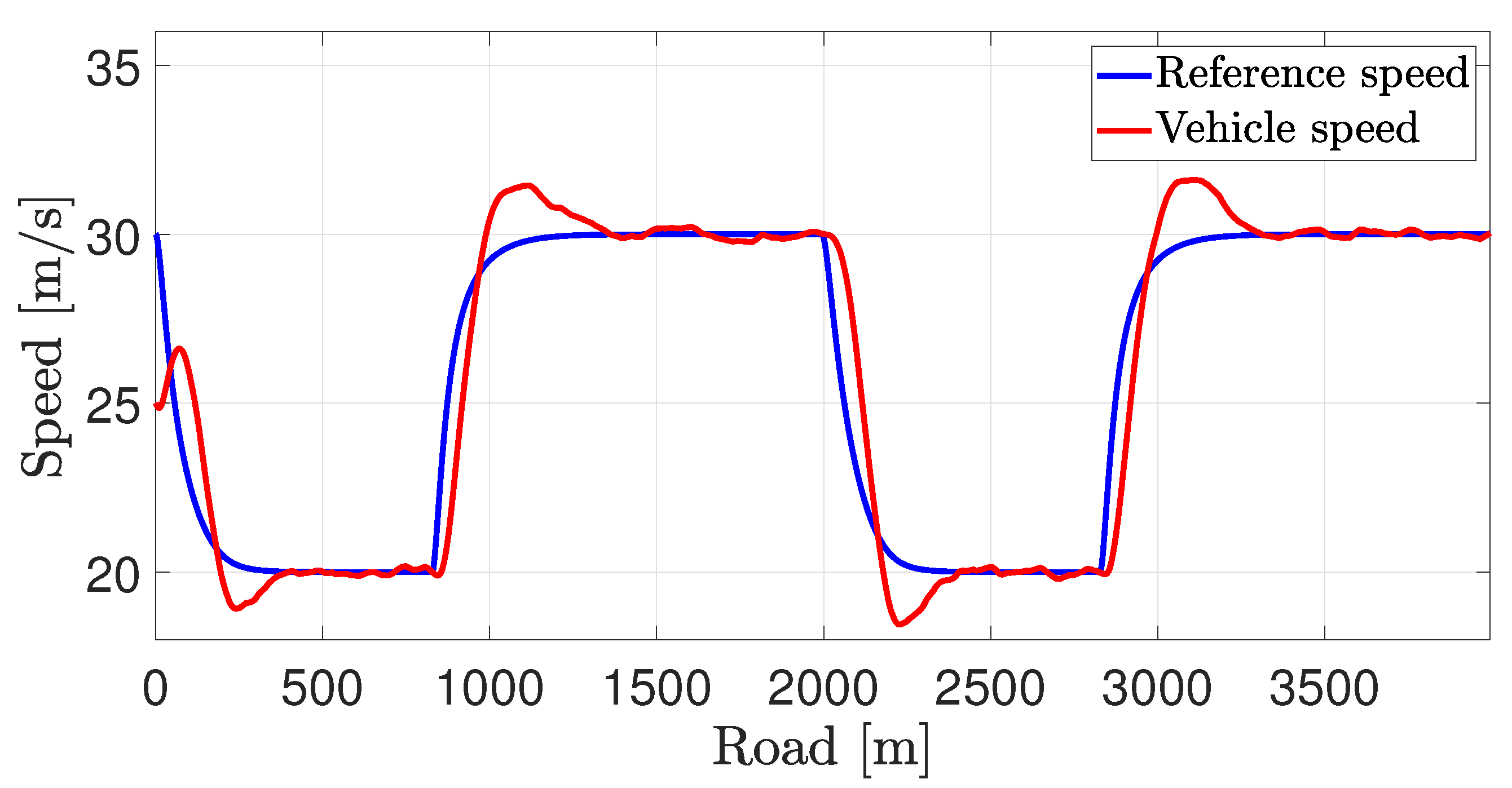
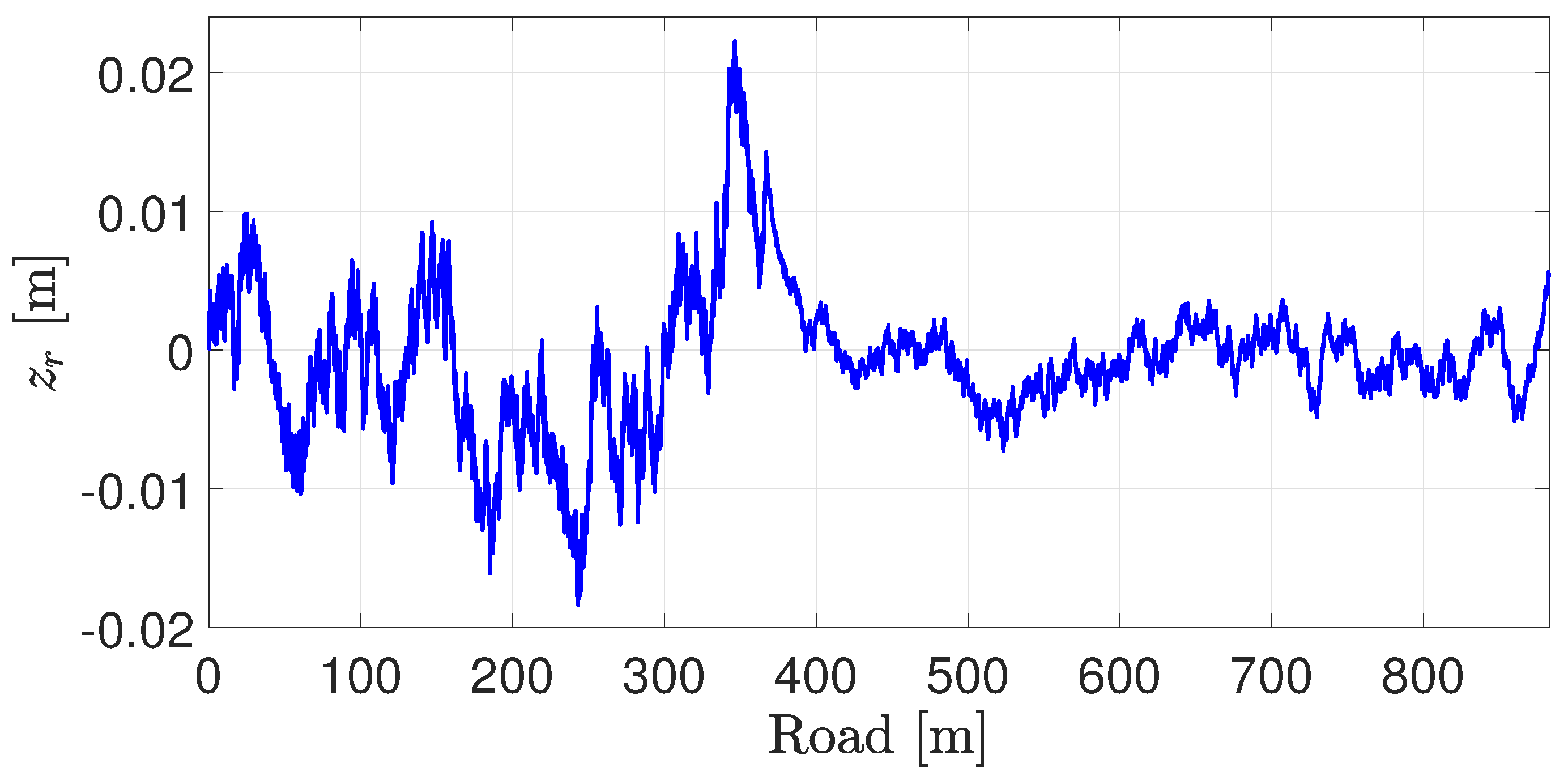
We see from Figure 20 that each time the road type or the desired RMS value changes, a new reference speed is calculated, and the cruise control effectively tracks this value. The resulting road displacement $z_r$ significantly increases after 36 s (around 1000 m) due to the change in road type (only the displacement at the front right corner of the vehicle is shown in Figure 21).

The resulting accelerations are shown in Figure 22, whose RMS values are $1.2360$ m/s${}^2$ for the passive suspension case and $0.4301$ m/s${}^2$ for the LPV ${\mathcal{H}}_2$ semi-active suspension case, which correspond to the comfort level of “uncomfortable” and “a little uncomfortable”, respectively, according to Table 3. These results show that the latter further improves driving comfort by limiting the acceleration transmitted to passengers. Finally, the resulting deflections are shown in Figure 23, from which we can see that semi-active suspension leads to smaller deflection values compared to passive suspension.

6.2. Simulation Scenario 2

The second simulation scenario is used to assess the robustness of the proposed approach w.r.t uncertainty on the sprung mass and viscous damping coefficients at the corners. This scenario is designed by adding the following uncertainty into the first one. The uncertain parameters are shown in

Table 5. Uncertain parameters.

Uncertain Parameter	Value
Sprung mass $m_s$ at each corner	315 + 2.5% kg
Viscous damping coefficients $c_{fl}$ and $c_{fr}$ at the front corners	3000 + 10% Ns/m
Viscous damping coefficients $c_{rl}$ and $c_{rr}$ at the rear corners	6000 + 10% Ns/m

.

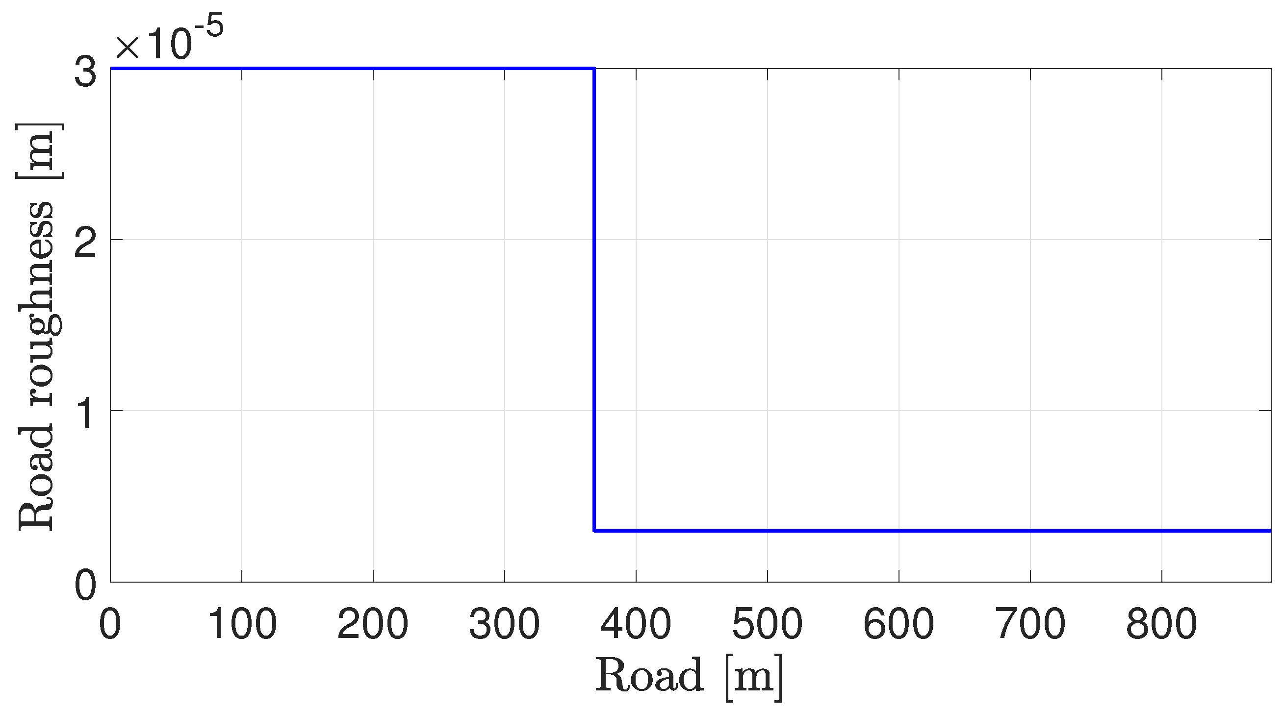
The total simulation time is 60 s. The simulation scenario is as follows (see Figure 24 and Figure 25):

• At 20 s (around 160 m), the desired comfort level (characterized by the given RMS acceleration) increases from 0.2 to 0.3 m/s${}^2$;
• At 40 s (around 360 m), the road type (characterized by the estimated road roughness) changes from B to A.

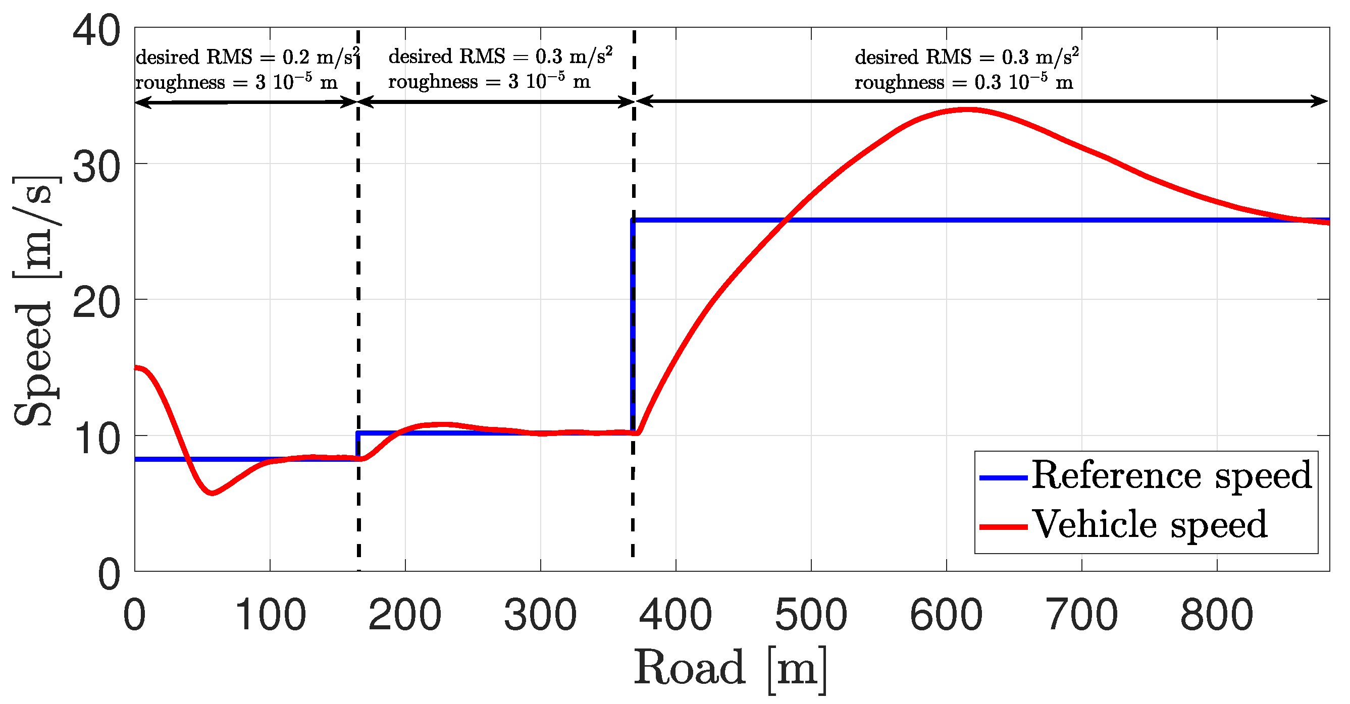
Again, we see from Figure 26 that the new reference speed is calculated, and the cruise control effectively tracks this value. The resulting road displacement $z_r$ significantly decreases after 40 s (around 360 m) due to the change in road type (only the displacement at the front right corner of the vehicle is shown in Figure 27).

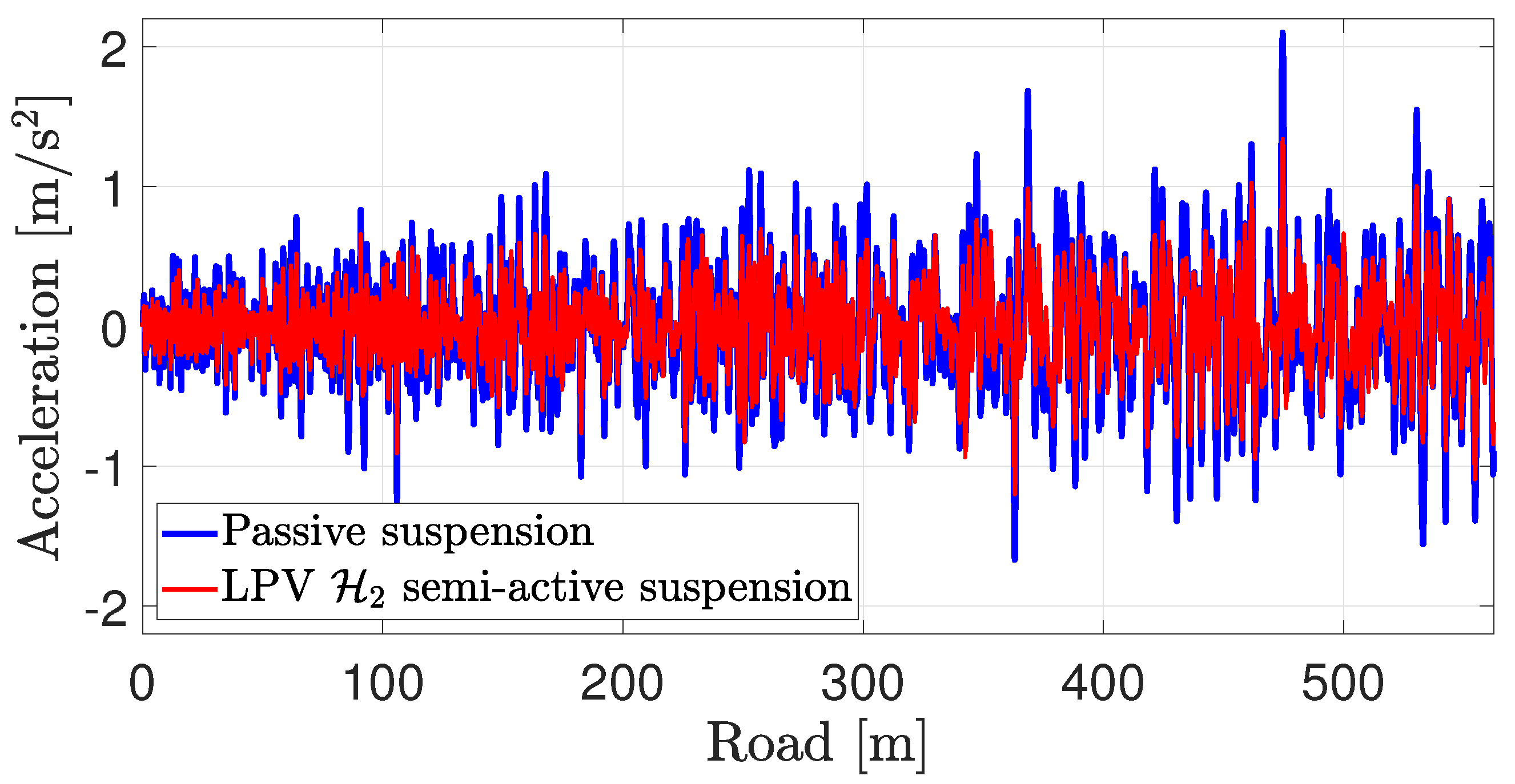
The resulting accelerations are shown in Figure 28, whose RMS values are $1.1947$ m/s${}^2$ for the passive suspension case and $0.6916$ m/s${}^2$ for the LPV ${\mathcal{H}}_2$ semi-active suspension case, which correspond to the comfort level of “uncomfortable” and “fairly uncomfortable”, respectively, according to Table 3. Finally, the resulting deflections are shown in Figure 29, from which we can see that again, semi-active suspension leads to smaller deflection values compared to passive suspension. These results show that the proposed method is robust enough w.r.t the uncertainty.

6.3. Comparison of Comfort Performances: Passive vs. Semi-Active Suspension

Table 6. RMS acceleration (m/s${}^2$).

Simulation Scenario	Passive Suspension	Semi-Active Suspension
Scenario 1	$1.2360$	$0.4301$
Scenario 2	$1.1947$	$0.6916$

summarizes the comfort evaluation for the two performed simulation scenarios.

Clearly, the LPV semi-active suspension control outperforms the passive one, and it allows for an efficient coupling between the longitudinal and vertical dynamics.

7. Conclusions

This work presented an integrated strategy for comfort-oriented vehicle cruise and suspension control with a robust/LPV approach in the ${\mathcal{H}}_2$ framework. We related driving comfort (quantified using the filtered sprung mass acceleration) and road type with the vehicle speed to obtain comfort-guaranteeing reference speed functions. We then designed a cruise and a semi-active suspension controller respectively for vehicle longitudinal and vertical dynamics, which are linked to each other through the vehicle speed as a scheduling parameter. These controllers were tested by performing simulations, first independently and then in an integrated framework using a nonlinear full-vehicle model validated from real data. Results showed that the vehicle was capable of finding a speed value guaranteeing comfort and tracking this value thanks to cruise control, while semi-active suspension control provided further enhancement of comfort level. Indeed, the integrated control approach was adapted to the comfort requirement and vehicle speed. It is worth mentioning that we relied on basic assumptions and a reasonable amount of knowledge of the environment, making this strategy realistic.