Abstract
Because the surface and submerged vehicles radiate Ultra-Low-Frequency (ULF) Electromagnetic waves, the status of the vehicles in the ocean can be detected and explored by analyzing such signals, and this has been gained increasing attention. In this paper, a hybrid algorithm of the ant colony algorithm and Levenberg–Marquardt algorithm is proposed to locate a moving target with a constant speed based on the fully investigation of the uniformly magnetized spheroid model. Additionally, an experiment has been conducted to validate the performance of the hybrid algorithm. At the same time, the comparison between the proposed ellipsoid model with the conventional dipole model has also been done, and the results show that the calculated results based on the prolate spheroid model agree well with the recorded GPS results with maximum 6.67% average error, which is way better than the dipole model (31.59%, max.).
1. Introduction
The increasing development of ocean exploitation and military applications has made the measurement and detection of surface or underwater vehicles’ physical signals significant. Due to its longer transmission capability, the ultrasonic technique has been widely applied for the detection of moving targets. However, the modern acoustic stealth techniques and harsh environments in shallow waters have been a major barrier for the acoustic detection methods [1,2]. Since Ultra Low Frequency electromagnetic signals (0–3 Hz) are radiated by the moving objects in the sea, such signatures have been paid attention to and studied by the military and academic fields for a long time [3]. In the past, the inductive loops were used to prevent submarines intrusion, which would be installed in the protected ports, harbors, and other important spots [3]. Meanwhile, numerous studies have been devoted to the investigation of the field sources of the underwater targets, such as submarine, unmanned underwater vehicle (UUV), etc. [4,5]. With the development of the integrated technologies, the performance of electric/magnetic sensors have been hugely improved, which would enable the portable sensor deployed in the required spots where the magnetic anomaly detection (MAD) systems installed on the unmanned air vehicles (UAVs) were proposed [6]. In the near future, the envisioned swarms of the UAVs with MAD systems would make it practical for the large shallow sea monitoring and acoustically quiet submarine detection [7].
Because of the small size, magnetic sensors are commonly adopted, which makes the development of the magnetic detection technologies stable [8]. Furthermore, traditional building materials of the vehicles such as steel and iron are magnetized due to magnetization effects if they stay in the geomagnetic field environment for a long time, which introduces the additional magnetic field. A study shows that the ship’s magnetic field can be approximated as a static magnetic field [9], and this would add one more dimension of the detectable signals. By analyzing the magnetic field signal radiated by the vehicles, the state of the target’s movement can be estimated. However, a suitable target magnetic field model should be carefully chosen, the most common of which is the single magnetic dipole [10] or the horizontal electric dipole [11]. Additionally, other models, such as the single uniformly magnetized spheroid model (referred to as the single ellipsoid model), the magnetic dipoles array model, and the hybrid model of the single ellipsoid model and dipoles array (abbreviated as the hybrid model) were also proposed and studied [12], where the single ellipsoid model has fewer parameters and lower requirements for the amount of information at the measuring points. Furthermore, numerous spheroid vehicles have been applied in the realistic operational environment [13,14], while Ref. [15] investigates the design, construction, and implementation of a novel spherical unmanned underwater vehicle prototype for operations navigating confined, entanglement-prone marine environments. The application of such vehicles would emphasize the studies of the spheroid model. In addition, the stability of the model can be guaranteed even when there is not much effective information at the measuring points. Furthermore, it should be pointed out that the objects cannot be effectively equivalent to the magnetic dipole model at a close range [16]. Thus, numerous studies have been conducted on the single ellipsoid model. Ref. [17] compared two structure models and evaluated their performance. In addition, Ref. [18] later used a single rotation elliptic sphere magnetic model to locate the warship. However, to realize these methods, repeatable measurements should be done at various measuring points to achieve the required accuracy, which is hard to realize in the battle field. In addition, such operations would need numerous sensors to build a network which would increase the cost and the problems of synchronization and installation in the sea. To achieve a rapid location speed, a method using only one three-axis fluxgate magnetic sensor is proposed based on the prolate spheroidal model here in this manuscript, which is the main contribution of our work. This is therefore the originality. Meanwhile, a hybrid optimization algorithm is proposed which combines both the ant colony algorithm and the Levenberg–Marquadt algorithm. In addition, experiments on the real ship localization are conducted to verify the localization performance of the single ellipsoid model in the near magnetic field environment. At the same time, the comparison of the ellipsoid model to the dipole model is conducted, and the results show that the proposed model outperforms the traditional dipole one.
2. Methods
2.1. Target Modeling
Generally, the ship can be approximately modeled as a prolate spheroid one, shown in Figure 1 [16]. The semi-major axis of the ellipsoid can be taken as half the length of the ship (L is the length of the ship), and the semi-minor axis of the ellipsoid can be taken as half the width of the ship (B is the maximum ship width of the ship). The coordinate system is established with the center of the ship as the origin, where the x-axis direction as the longitudinal direction and the z-axis as vertical downward. The ellipsoid is uniformly magnetized along three coordinate directions in the terrestrial magnetic field, and its corresponding magnetic moment is . Thus, the magnetic field generated at the measuring point is:
where are the calculation coefficients of the ellipsoid magnetic fields, which are the known spatial distribution functions and are calculated as follows:
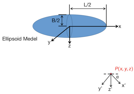
Figure 1.
Schematics of the uniformly Magnetized spheroid model of the vehicle.
Place the sensor at the measuring point P and the coordinate system of the measuring point is also shown in Figure 1, where the z’ axis is vertically downward while the angle between the x’ axis and the target heading, i.e., the x-axis, is . Assuming that the target moves in a straight line at a uniform speed along the x-direction, while the speed is v, and the sampling interval is . Supposed that the speed of the target does not change when the target passes for a short time. Then, the relationship between the j’s output of the sensor (i.e., the target’s radiated magnetic fields) is:
where , and for a magnetic target with a fixed direction of movement, is a fixed value.
Suppose the coordinate center position of the ship during the j sampling is , and the coordinates at the sampling is :
When the target passes the receiving point, the sensor samples m times to obtain m sets of the three-component data. Using these m sets of sampling data, the linear equations of the model can be established:
where F is the coefficient matrix about the target position. M is the magnetic field model parameter. H is the target magnetic field.
To summarize, the ship magnetic localization problem can be seen as the optimization problem of solving the following nonlinear unconstrained equation:
The objective function E is a nonlinear function of , which would lead to a typical nonlinear optimization problem.
2.2. Hybrid Localization Algorithm
In order to solve the above-mentioned nonlinear optimization problem, a hybrid localization algorithm can be used which combines ant colony algorithm and Levenberg–Marquardt algorithm, where both advantages of the global search optimization ability of ant colony algorithm and the local accurate search ability of Levenberg–Marquardt algorithm can be taken to achieve a better performance. For the combined localizaiton algorithm, the ant colony algorithm is used to obtain the initial rough solution, which would be transferred to the Levenberg–Marquardt algorithm to obtain the final optimal solution.
The Levenberg–Marquardt algorithm can be written as:
When increases, the algorithm is close to the steepest descent method of small learning speed:
where .
It can be easily seen that, when drops to 0, the algorithm becomes the Gauss–Newton method.
The ant colony algorithm follows the below operations in each iteration [19]: a group of ants move between adjacent states of the problem synchronously or asynchronously. They gradually construct a feasible solution to the problem by using the pheromone, the heuristic information associated in each state, and the state transition rule selects the direction of movement; when each ant constructs the solution, the pheromone can be updated locally; after all the ants have completed the construction of the solution, the pheromone is updated globally according to the obtained solution. The iterative process continues until a certain stopping condition is met. Common stopping conditions are the maximum running time or the maximum number of solutions allowed to be constructed.
The structure of the algorithm is shown in Algorithm 1. It should be pointed out that the ant colony algorithm is easy to stagnate in the later stage of the operation because of its inability of fine search in local areas; thus, the iteration number and the ant number should be appropriately shortened in order to improve the efficiency.
| Algorithm 1: Hybrid Localization Algorithm |
| Require: |
| Require: Ant Colony Algorithm: set |
| 1: loop |
| 2: for |
| 3: loop |
| 4: for |
| 5: update Equation (4), do |
| 6: end loop |
| 7: update |
| 8: end loop |
| 9: Find to minimize |
| Require: LM Algorithm: set , Maximum Iteration Number N, Minimum Error |
| 10: for , do |
| 11: loop |
| 12: update Equation (8) |
| 13: update |
| 14: until |
| 15: end loop |
2.3. Description of the Validation Experiment
To validate the proposed method, an experiment was conducted in a wide sea area far away from the channel in Sanya, where there is almost no influence from the other objects. The depth of the experimental sea is 26 m, while the experimental area is 2.6 km long and 1.1 km wide. The ship used in the experiment is Haihong No. 1, shown in Figure 2, which is 54 m long and 13.2 m wide.
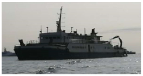
Figure 2.
Photo of the experimental ship.
The experimental equipment mainly includes a three-axis high-precision fluxgate sensor, a high-precision attitude sensor, a data acquisition storage module, and a power supply battery, as shown in Figure 3. The high-precision attitude sensor is used to convert the magnetic field data collected by the fluxgate to the geographic coordinate system when the ship passes, while the data acquisition storage module records the magnetic field data and attitude data in real time for the subsequent processing.
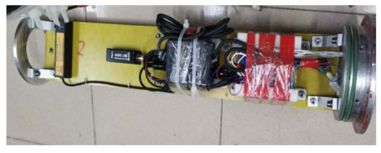
Figure 3.
Photo of the experimental equipment with one three-axis fluxgate magnetic sensor.
Since the geomagnetic field can be regarded as stable, the sinking equipment can work for a while to collect the geomagnetic field. Then, the target’s magnetic field can be obtained by subtracting the geomagnetic field from the recorded data when the ship passes. The schematic of the experiment is shown in Figure 4. From the figure, we can see that the ship would sail at a constant speed v along the planned lines, and the experiment would repeat at different distance abeam D: 0 m, 10 m, 20 m, 30 m, 40 m, and 50 m at the speed of 8 knots. The GPS system is used to record the required data to ensure that the trajectory of the ship meets the preset requirements and also is set as the standard for our algorithm. Light wind is acceptable to make sure the target can move as planned, and this would also assure that the sea depth would not change a lot because it can be used as a reference to evaluate the performance of the method, which would be discussed in Section 4.
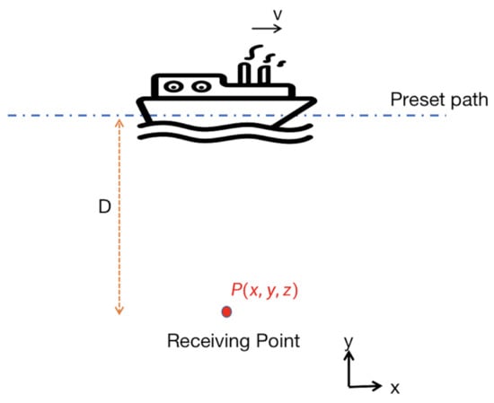
Figure 4.
The schematic of the experimental survey line (top view).
3. Results
Since the ship moves along the x-direction at a fixed speed shown in Figure 4 the position change in the x-direction should be an inclined straight line with the slope of the ship’s sailing speed on the time axis, and there is basically no change in the y and z directions. The localization result is shown in Figure 5, where the upper 3 are the received magnetic field and the lower 3 are the localization results. From the figure, it can be seen that the time node at which the localization results have been significantly improved appears at approximately 0 m in the x-direction when the ship is closest to the magnetic sensor to make the magnetic field signals the strongest. In the later stage of the algorithm, the localization distance in the y-direction converges to around 12.5 m, and the localization distance in the z-direction converges to around 25.2 m, which are in good agreement with the actual situation. However, in the initial period, when the ship is far from the sensor, the magnetic field signal is weak to make the noise-to-signal ratio non-neglectable, which has a greater impact on localization. As the ship gets closer to the magnetic sensor, the target magnetic field signal gradually increases, leading to the increase of the signal-to-noise ratio to make more magnetic field data effective, thus the localization result will gradually get better.
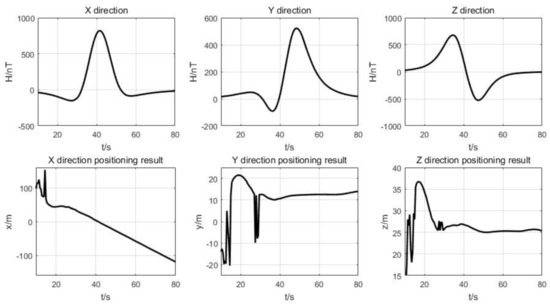
Figure 5.
Received signals and the output location when the distance abeam D is 10 m.
Different measuring lines with various distance abeam are also conducted to evaluate the proposed method. The calculation formula for the relative error between the real value and the algorithm calculation value is as follows:
where is the preset value and is the calculated value.
The localization results in the y-direction are shown in Table 1, and the localization results in the z-direction are shown in Table 2. Both results agree with the recorded data, but there are some some discrepancies in the y-direction. It is mainly due to the measurement errors of the GPS system. Additionally, it can be easily seen that the z-direction results agree well since the depth of the sea would remain at a constant value.

Table 1.
Localization results in the y-direction for different distance abeams.
Table 2.
Localization results in the z-direction for different distance abeams.
4. Discussion
The localization results of the ellipsoid model and the single dipole model at a distance abeam of 30 m are also compared, the results of which are shown in Figure 6. From the figure, it can be easily seen that the ellipsoid model would converge to the preset values when the magnetic dipole model still has a large deviation. Because the real value of the sea depth would not change a lot, the localization results of the z-direction from both source models are illustrated in Table 3. We can see that the spheroid source model is better than the magnetic one with the largest difference of 1.86 m to 12.01 m respectively. The corresponding relative errors from Equation (9) are and , which validates the proposed assumption that the spheroid source model is better than the magnetic dipole model at the near area localization.
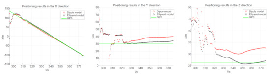
Figure 6.
Comparison of the spheroid model with the magnetic dipole model to the recorded GPS value when the distance abeam is 30 m. “GPS” represents the recorded GPS value. “Dipole model” represents the calculated results of the dipole model. “Ellipsoid” represents the calculated results of the ellipsoid model.
Table 3.
The comparison of Localization results in the z-direction between magnetic dipole model and ellipsoid model for different distance abeams (the sea depth is 26 m).
5. Conclusions
A novel magnetic localization method only using one measuring point data is introduced and studied in the paper, where a new hybrid method is investigated based on the full study on the uniformly magnetized spheroid model. An experiment has been conducted to validate the proposed method, and the comparison of recorded data with the calculated one shows the good performance of the proposed ellipsoid model with an average error around 6.67%. At the same time, the study shows that the prolate ellipsoid model can outperform the traditional dipole model, which would pave the road to the wide application of the ellipsoid model in localisation. Furthermore, more experiments with various vehicle types should be conducted to enrich the study.
Author Contributions
Conceptualization, K.Y. and B.L.; methodology, K.Y. and B.L.; software, D.L.; validation, D.L., K.Y. and B.L.; formal analysis, K.Y.; investigation, K.Y. and B.L.; resources, B.L.; data curation, D.L.; writing—original draft preparation, D.L. and K.Y.; writing—review and editing, K.Y.; visualization, D.L. and K.Y.; supervision, K.Y. and B.L.; project administration, K.Y.; funding acquisition, K.Y. and H.L. and K.D. All authors have read and agreed to the published version of the manuscript.
Funding
This research was funded by NFSC Grant No. 61901386 and by Long-term Funds of Science and Technology on Near-Surface Detection Laboratory Grant No. TCGZ2020C002.
Conflicts of Interest
The authors declare no conflict of interest.
References
- Tan, H.P.; Diamant, R.; Seah, W.K.; Waldmeyer, M. A survey of techniques and challenges in underwater localization. Ocean. Eng. 2011, 38, 1663–1676. [Google Scholar] [CrossRef]
- Liang, G.L.; Lin, W.; Wang, Y. Estimation of effective sound velocity in shallow channel and its application in underwater acoustic localization. Technical Acoustics. Tech. Acoust. 2012, 31, 42–47. [Google Scholar]
- Holmes, J.J. Exploitation of a Ship’s Magnetic Field Signatures. Synth. Lect. Comput. Electromagn. 2006, 1, 1–78. [Google Scholar] [CrossRef][Green Version]
- King, R.W.P. Lateral electromagnetic waves from a horizontal antenna for remote sensing in the ocean. IEEE Trans. Antennas Propag. 1989, 37, 1250–1255. [Google Scholar] [CrossRef]
- Sun, F.; Huang, Y.; Wu, L.-H. Underwater Continuous Localization Based on Magnetic Dipole Target Using Magnetic Gradient Tensor and Draft Depth. IEEE Geosci. Remote Sens. Lett. 2013, 11, 178–180. [Google Scholar]
- Tiron, R. Gulf Nation Poised to Lead Region in Production of Unmanned Aircraft. Scand. J. Rheumatol. 2005, 35, 44–47. [Google Scholar]
- Holmes, J.J. Reduction of a Ship’s Magnetic Field Signatures. Synth. Lect. Comput. Electromagn. 2006, 1, 1–78. [Google Scholar] [CrossRef][Green Version]
- Gao, X. Research on the Localization of Alternating Magnetic Dipole Source in Geomagnetic Environment. Ph.D. Thesis, Northwestern Polytechnical University, Xi’an, China, 2018. [Google Scholar]
- Ye, P.; Gong, S. Ship’s Physics Field; Ordnance Industry Press: Beijing, China, 1992. [Google Scholar]
- Gao, X.; Yan, S.; Li, B. Study of hybrid algorithm for localization of mobile magnetic target by a single fluxgate. J. Dalian Univ. Technol. 2016, 56, 292–298. [Google Scholar]
- Jinhong, W.; Bin, L.; Lianping, C.; Li, L. A Novel Detection Method for Underwater Moving Targets by Measuring Their ELF Emissions with Inductive Sensors. Sensors 2017, 17, 1734. [Google Scholar]
- Qu, X.; Yang, R.; Shan, Z. Analysis and comparison on magnetic field modeling method of submarine. Ship Sci. Technol. 2011, 33, 7–11. [Google Scholar]
- Milosevic, Z.; Fernandez, R.A.S.; Dominguez, S.; Rossi, C. Guidance for Autonomous Underwater Vehicles in Confined Semistructured Environments. Sensors 2020, 20, 7237. [Google Scholar] [CrossRef] [PubMed]
- Sands, T. Development of Deterministic Artificial Intelligence for Unmanned Underwater Vehicles (UUV). Mar. Sci. Eng. 2020, 8, 578. [Google Scholar] [CrossRef]
- Eldred, R.; Lussier, J.; Pollman, A. Design and Testing of a Spherical Autonomous Underwater Vehicle for Shipwreck Interior Exploration. Mar. Sci. Eng. 2021, 9, 320. [Google Scholar] [CrossRef]
- Holmes, J.J. Modeling a Ship’s Ferromagnetic Signatures. Synth. Lect. Comput. Electromagn. 2006, 1, 1–78. [Google Scholar] [CrossRef][Green Version]
- Li, H.; Li, Q.; Liu, J. Comparison between the Two Models of Warship’s Magnetic Field. J. Detect. Control. 2007, S1, 62–66. [Google Scholar]
- Bian, X.; Li, Q.; Li, H. Study on real-time Magnetic localization Methods of Warship. J. Detect. Control. 2006, 28, 3538. [Google Scholar]
- Vázquez, K.R. Ant Colony Optimization. Genet. Program. Evolvable Mach. 2005, 6, 459–460. [Google Scholar] [CrossRef]
Publisher’s Note: MDPI stays neutral with regard to jurisdictional claims in published maps and institutional affiliations. |
© 2021 by the authors. Licensee MDPI, Basel, Switzerland. This article is an open access article distributed under the terms and conditions of the Creative Commons Attribution (CC BY) license (http://creativecommons.org/licenses/by/4.0/).