Proposal of a Decoupled Structure of Fuzzy-PID Controllers Applied to the Position Control in a Planar CDPR

Abstract

The design of robot systems controlled by cables can be relatively difficult when it is approached from the mathematical model of the mechanism, considering that its approach involves non-linearities associated with different components, such as cables and pulleys. In this work, a simple and practical decoupled control structure proposal that requires practically no mathematical analysis was developed for the position control of a planar cable-driven parallel robot (CDPR). This structure was implemented using non-linear fuzzy PID and classic PID controllers, allowing performance comparisons to be established. For the development of this research, first the structure of the control system was proposed, based on an analysis of the cables involved in the movement of the end-effector (EE) of the robot when they act independently for each axis. Then a tuning of rules was carried out for fuzzy PID controllers, and Ziegler–Nichols tuning was applied to classic PID controllers. Finally, simulations were performed in MATLAB with the Simulink and Simscape tools. The results obtained allowed us to observe the effectiveness of the proposed structure, with noticeably better performance obtained from the fuzzy PID controllers.

1. Introduction

In recent years, research in the field of robotics has focused on the study of cable-driven parallel robots (CDPR), with the control stage being very important, and involving a significant choice in the structure of the robot. In this way, in [1], the control of a CDPR to simulate movements of a satellite, allowing experimentation with a vibration control caused by external disturbances and by autorotation is developed. Additionally, in [2], a coordinated dynamic control in the task space (CDCT) was proposed for a CDPR to guarantee high-precision control. By analyzing the contour error, a new timing error was introduced to represent the coordination relationship between axes, and an additional robust compensation using the defined timing error was designed. In [3], a robust torque control scheme for a CDPR based on a PD controller was designed with real-time mass estimation and path compensation for pick-and-place tasks with different masses. In [4], the use of a CDPR for 3D printing with concrete was reported. The proposed concept was used to test the possibility of constructing a house with high precision and a stable trajectory. In [5], a review of the state of the art of fully constrained cable-actuated parallel mechanisms and cable-suspended parallel mechanisms was presented, recalling the basic kinematic architecture and briefly exposing the associated static and kinematic models. For its part, in [6], a prototype CDPR was used to 3D print a wall made of glass powder for an artistic exhibition. The position of the robot was measured by 3 on-board lidars and its operation over 174 working hours was evaluated. Additionally, in [7], the application of a CDPR as a 3D printer was proposed, using a retractable end-effector to avoid the collision of the cables with the printed objects and to increase the working space, with a stiffness analysis of the disturbance present in the end-effector.

While the mathematical modeling of the mechanism is relatively complex due to the non-linearities of the components that make it up, such as cables and pulleys, empirical tuning controllers can be chosen, among them the fuzzy and classic PID. That is the case reported in [8], where a fuzzy control was used with an adaptive feedback method for non-linear systems, the controller helps the following error tend towards zero. In [9], a Sugeno-type controller was used for the independent design of the controller and the fuzzy observer. This was achieved through the development of a separation property which obtained satisfactory results from the non-linear systems. For its part, in [8], a fuzzy controller was coupled to highlight the characteristics of a PID controller, improving both the transient and steady-state responses [10]. Fuzzy controllers were also applied for speed and direction control in [11], where an investigation of fuzzy speed control was carried out for a frequency inverter connected to a permanent magnet (PM)-synchronous motor, where fuzzy logic was used based on the speed error. Other applications are in the area of mobile robots, as in [12], where fuzzy control rules were used to heuristically adjust the angles of the wheels and the data from an encoder used in the balance and drive of the mechanical wheel of a ball robot. Something similar was proposed in [13], where a fuzzy controller was used to control the speed and direction of an intelligent mobile robot that tracked and obtained the trajectory of a specific target. While in [14], a fuzzy adaptive PI controller for the non-linear control of the motion of a four-wheeled omnidirectional mobile robot was employed, the fuzzy adaptive algorithm adjusted the PI controller’s parameters, and the fuzzy inference rules were set using the tracking error and its derivative.

Several articles analyze ways to tune and apply a classic PID. In [15] the three main control effects were examined for the experimental or calculated values of the delay and the unit reaction rate of the process to be controlled. In [16], a controller based on a classical PID was designed and simulated to regulate the position and orientation of a six degrees-of-freedom (DOF) quadrotor. The control parameters were obtained according to the simulation results. In [17], some rules for the adjustment of the PID of a two-DOF robot manipulator were proposed. This adjustment procedure was extracted from the stability analysis using a Lyapunov function and the LaSalle invariance principle. Finally, in [18], the semi-global stability of robotic manipulators under classical PID control was demonstrated. Based on model compensation techniques, the non-linearities were grouped into a single function and are estimated using a reduced-order observer.

Prior to the control stage, a trajectory planner is required. In [19], the dynamic path planning (DPP) of a planar robot arm was described, non-heuristic algorithms to plan collision-free trajectories with information obtained from the environment by feedback. In the case shown in [20], a Catmull-Rom spline-based path planning scheme was proposed, which allowed a robot to move through several points with a method of speed limitation used at the beginning and end of each node, optimized through time scaling to keep speed and acceleration separated. Finally, in [21], a CDPR was used to simulate underwater conditions on a humanoid robot planning a dynamic polygonal 6-1-6 trajectory, to set the necessary speed and acceleration of the system tracking the humanoid robot.

For the most part, the research and design of control strategies in CDPRs involve the mathematical model, which demands effort in its modeling due to the non-linearities incorporated in the components of the mechanism. From the foregoing, it is important to have alternatives for controller structures that are easy and fast to tune and implement. With the aim of contributing to the field of CDPR control, a decoupled control structure proposal based on fuzzy PID and classic PID controllers was developed and studied, the results were analyzed and their performance was evaluated. The effectiveness of the fuzzy PID controller is demonstrated as having better tracking and less error compared to the classic PID. The main contribution of this research is to provide a decoupled structure for the position control of a CDPR requiring almost no mathematical analysis. The novelty consists in using a well-known design technique for controllers acting independently to control the position of the CDPR in each axis, which has not been previously reported in the literature.

The paper is structured as follows: in Section 2, the structure and equations of forces of the CDPR are presented, as well as the topology of the position control and trajectory planning. The tuning of the PID controller and the design of the fuzzy controller are also developed. In Section 3, the operation of PID and fuzzy PID controllers are simulated and the results are compared. In Section 4, a discussion on the obtained results is presented and, conclusions are established finally, in Section 5.

2. Materials and Methods

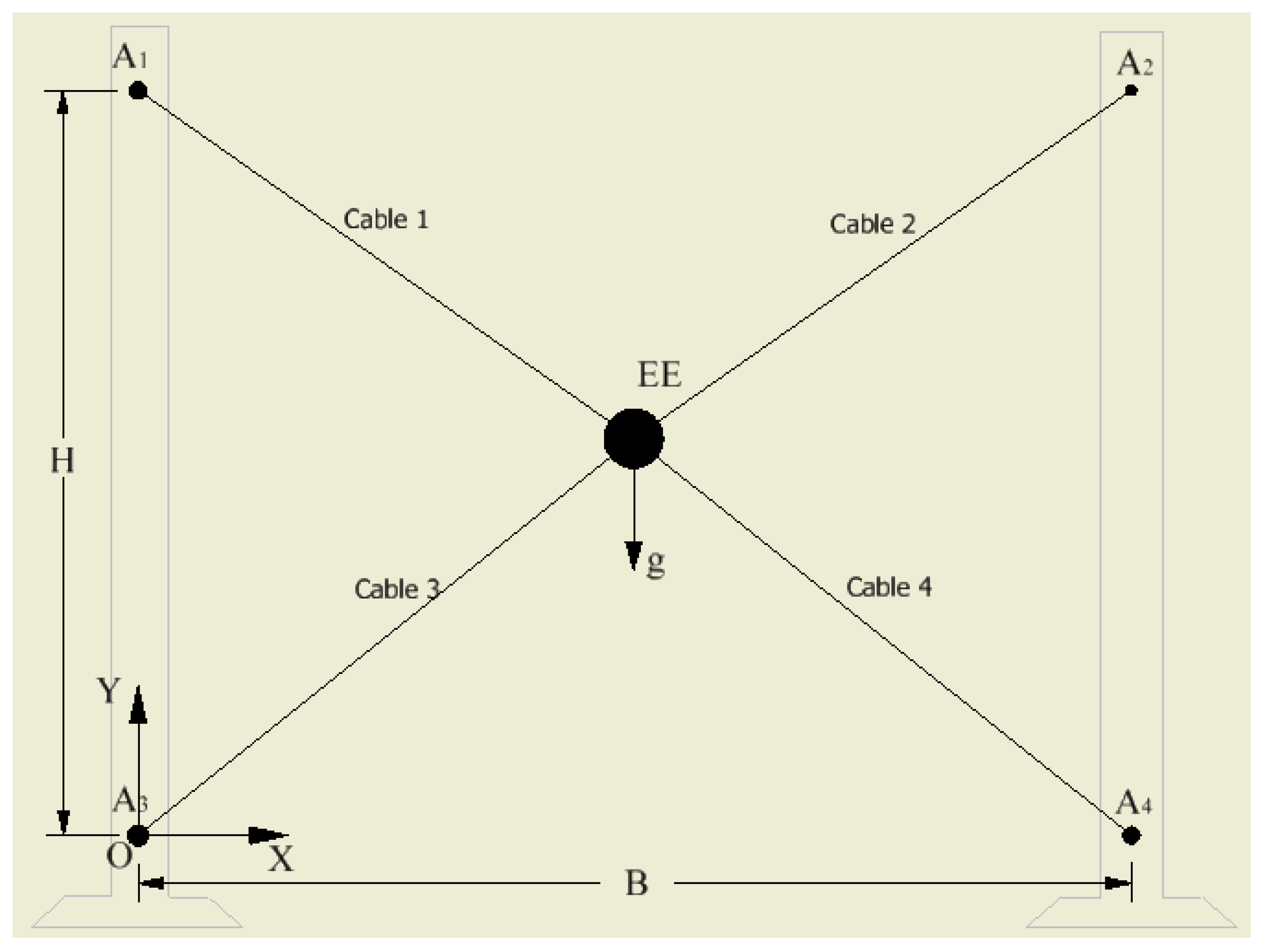
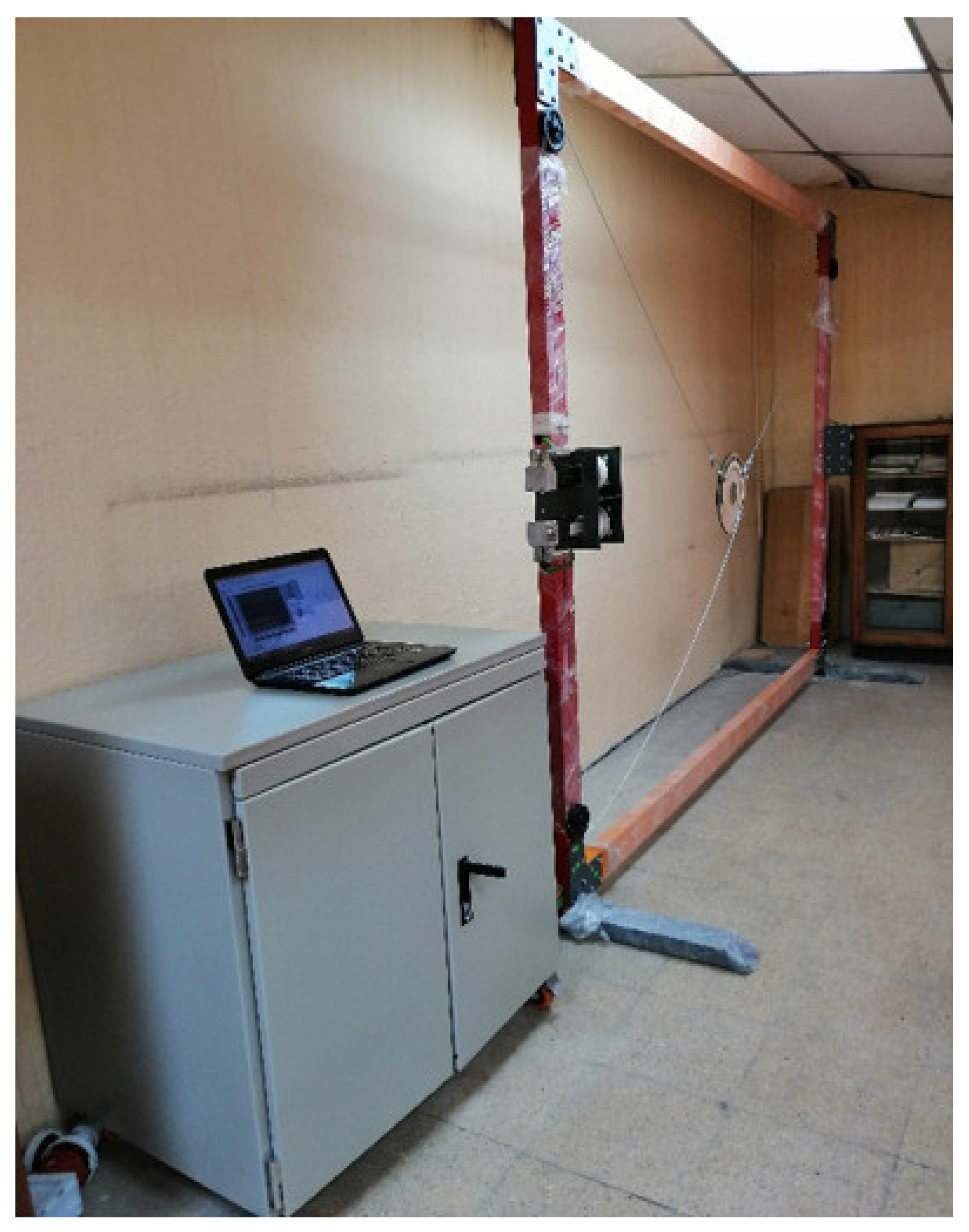
2.1. Structure of the Parallel Cable Mechanism

The planar CDPR mechanism shown in Figure 1 is made up of a fixed structure with two posts, and a mobile effector to which the cables are anchored allows for the application of force to generate movement in the vertical plane.

In Figure 1, A1, A2, A3, and A4 are the anchor points on the fixed structure, EE is the anchor point on the end-effector, B is the robot base, defined as the distance between the posts supporting the robot cables, and H is the robot height, defined as the height of the posts supporting the robot cables.

The robot workspace is delimited by the anchor points of the pulleys that guide the cable in the fixed structure. A hypothetical case of a mechanism with B = 3 m and H = 2.5 m, with an end-effector of 5 kg in weight and light nylon cables whose characteristics allow the robot to ignore catenary effects was considered [22].

The robot dynamic model is presented in Equation (1) through Equation (4) [23], which consider: the external forces at the EE, the weight of the EE, the friction damping forces of the environment where the robot works, and the forces developed in the robot cables.

$$f{d}_x-Bd·\dot{x_G}-{\displaystyle \sum }_{i=1}^4\left\{\left({\tau }_i-P_i\right)S_{ix}+Q_i{S}_{iy}\right\}=M{\ddot{x}}_G$$

(1)

$$f{d}_y+M\left(g·\mathrm{y}\right)-Bd·\dot{y_G}-{\displaystyle \sum }_{i=1}^4\left\{\left({\tau }_i-P_i\right)S_{iy}+Q_i{S}_{ix}\right\}=M{\ddot{y}}_G$$

(2)

where:

$$P_i={\rho }_m\left(L_i{g}^S-L_i{\ddot{L}}_i+\frac{1}{2}{\left(L_i{\dot{\alpha }}_i\right)}^2\right)$$

(3)

$$Q_i={\rho }_m\left(\frac{1}{2}{L}_i{g}^N-\frac{3}{4}{L}_i{\dot{L}}_i{\dot{\alpha }}_i-\frac{1}{3}{L}_i^2{\ddot{\alpha }}_i\right)$$

(4)

The different external forces and moments (wrenches) that affect the end-effector correspond to external forces ($fd$), gravitational forces ($M·g$), forces impressed on the effector due to its acceleration ($M·{\ddot{x}}_G,M·{\ddot{y}}_G$), and damping forces due to friction in the environment where the robot moves $\left(Bd·\dot{x_G},Bd·\dot{y_G}\right)$. The wires have constant density ${\rho }_m$, and are actuated by means of force ${\tau }_i$, ${\dot{L}}_i$ is recollection or extension speed, and ${\dot{\alpha }}_i$ is the angular speed of each wire. The speed of the cable’s center of mass in direction $S_i$ was considered. The robot model was developed in the MATLAB Simscape toolbox.

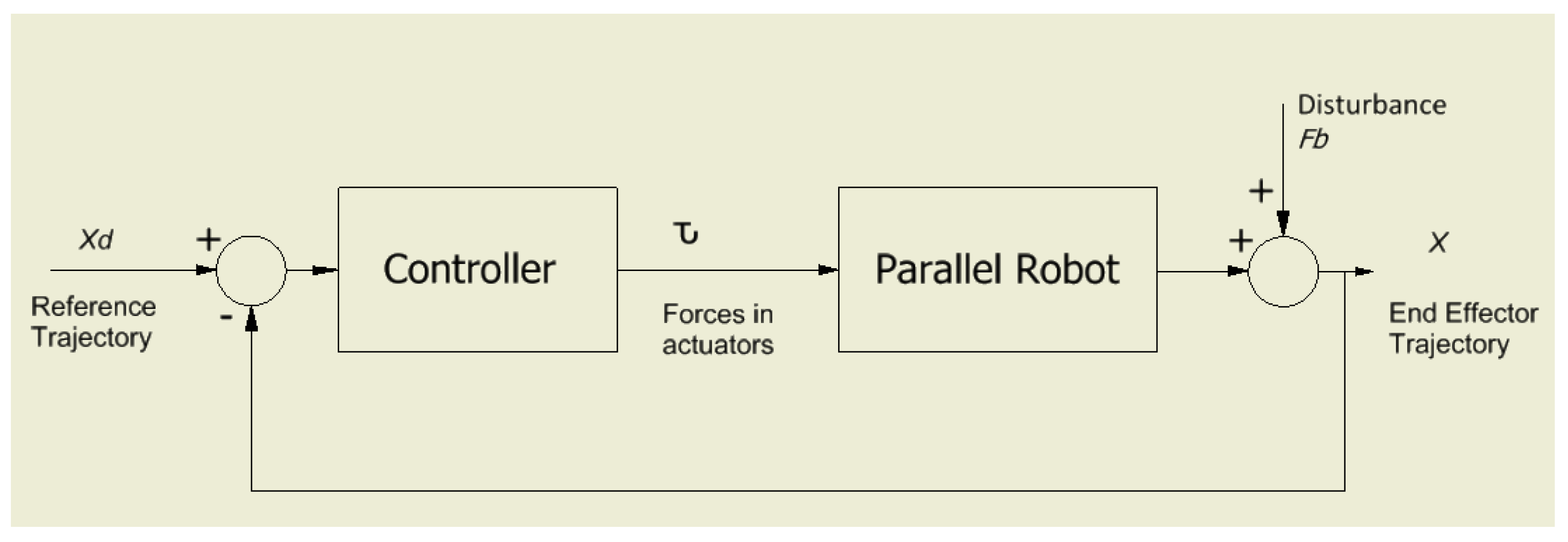
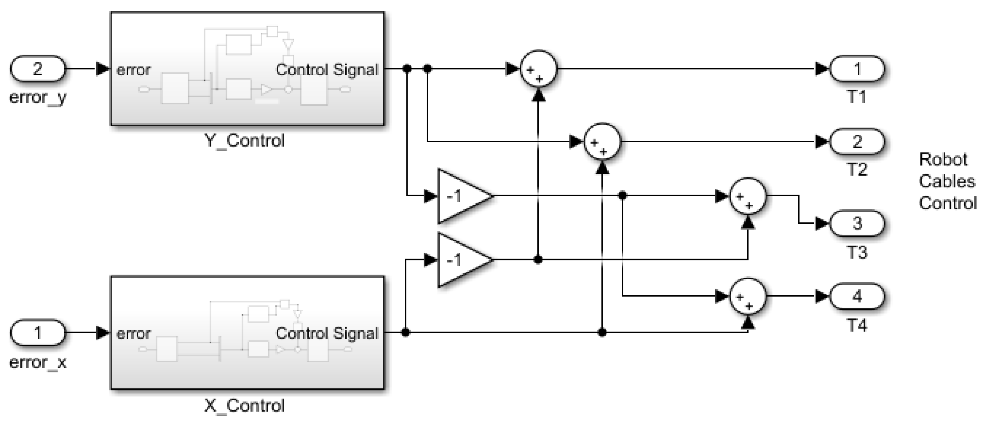
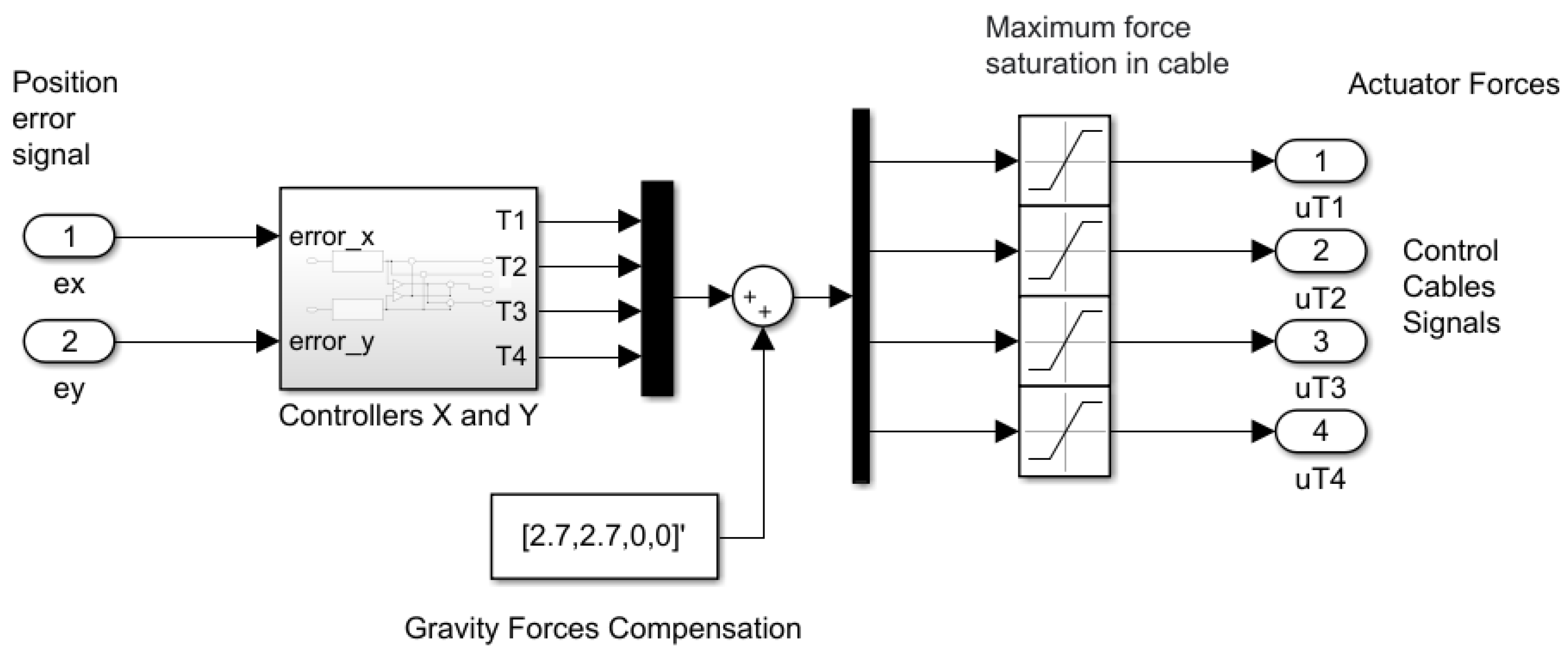
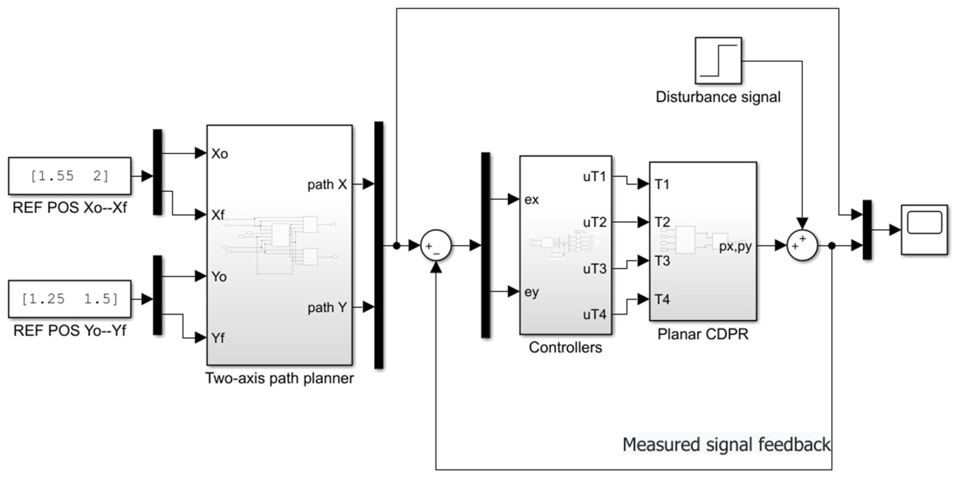
2.2. Motion Control Topology

Parallel robots are designed for various applications, among which are those where the end-effector does not exert contact or force with the environment, in which case a position control is required [24]. The position control of the robot can be approached in two ways, one referring to the joint space and the other to the task space. The choice of the control topology depends on the accessibility of the measurement of the signals and the demands of the robot application.

For position control in task space, the position of the end-effector is fed back directly. The control topology is shown in Figure 2, where the effect of a disturbance (representing a displacement in the position of the end-effector) is added for the purpose of evaluating the responses of the control system.

General control topologies used in robotics can be structured based on coupled or decoupled control schemes, as feasible [24].

For the case of the planar CDPR in Figure 1, a mixed controller structure was proposed for use in the task space under the following considerations:

• One controller performs the X-axis positioning control. For positive displacement, force is applied to cables 2 and 4, while for negative displacement, force is applied to cables 1 and 3.
• Another controller performs the Y-axis positioning control. For positive displacement, force is applied to cables 1 and 2, while for negative displacement, force is applied to cables 3 and 4.

The control structure for decoupled axis movement is shown in Figure 3, where the X-axis controller and the Y-axis controller are implemented as decoupled controllers with independent tuning.

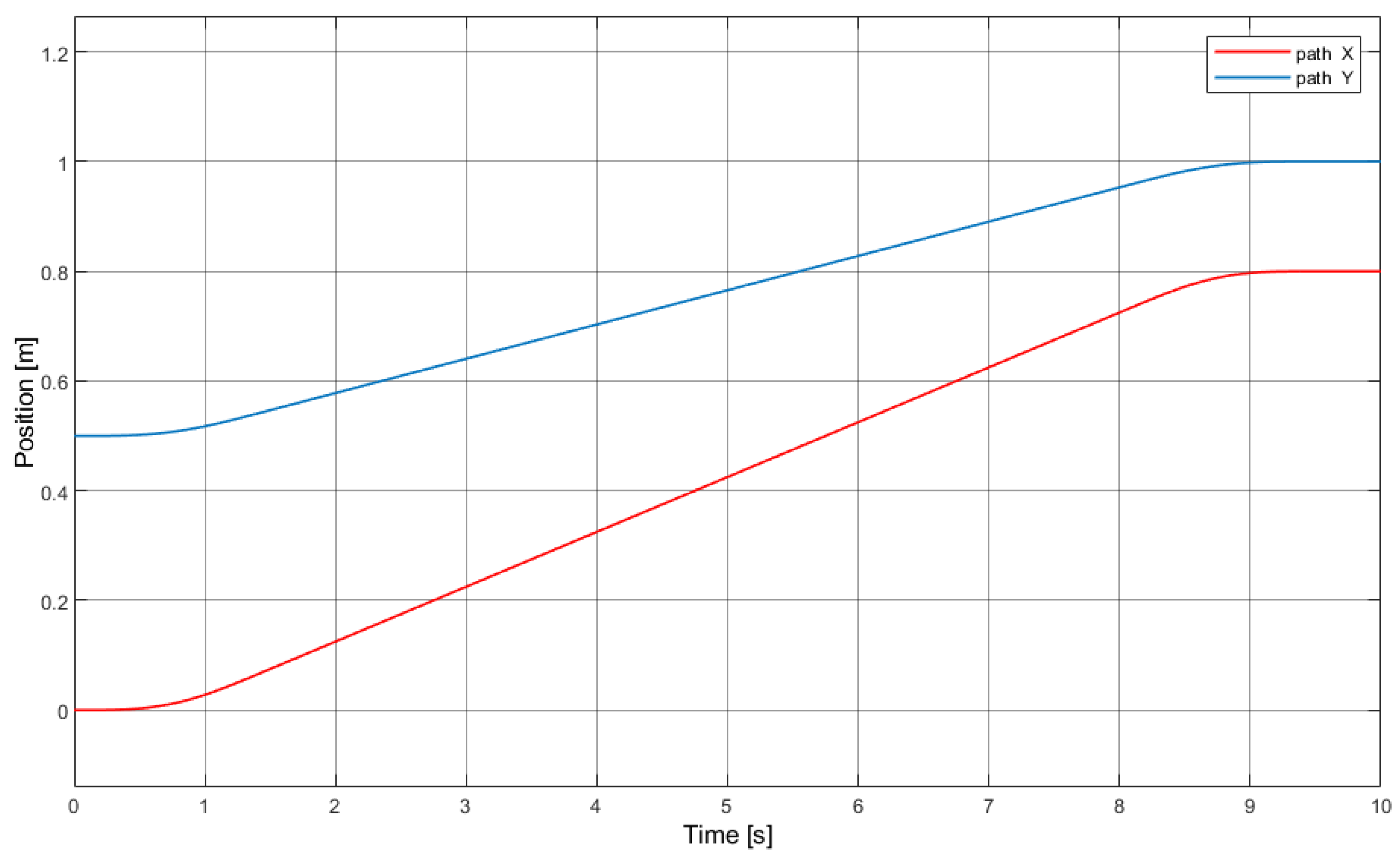
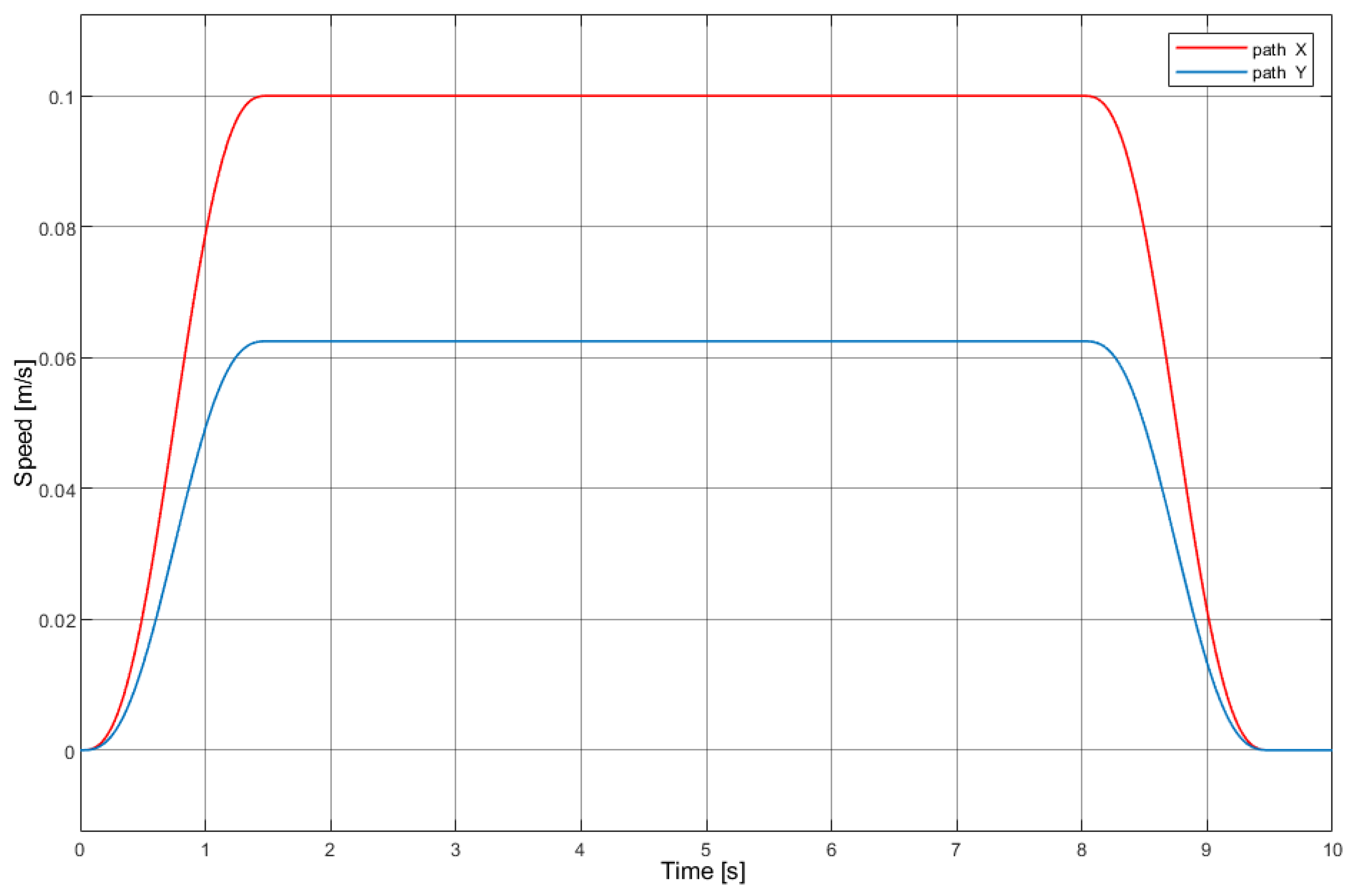
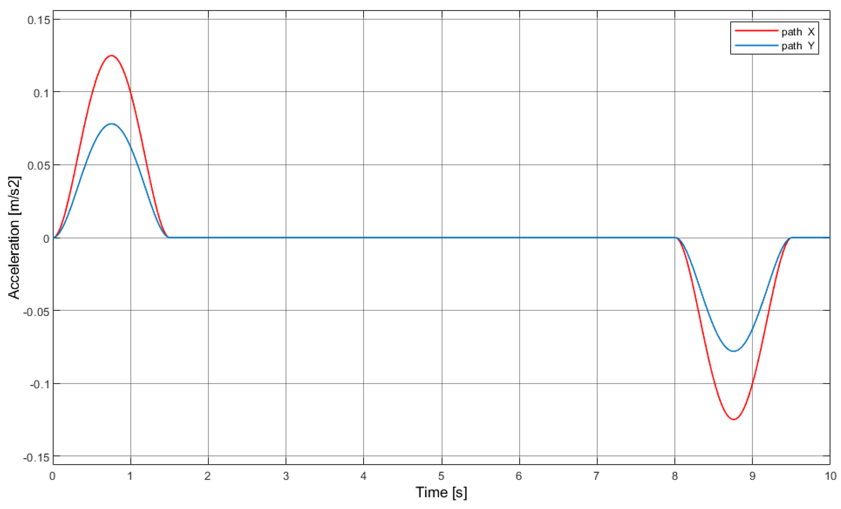
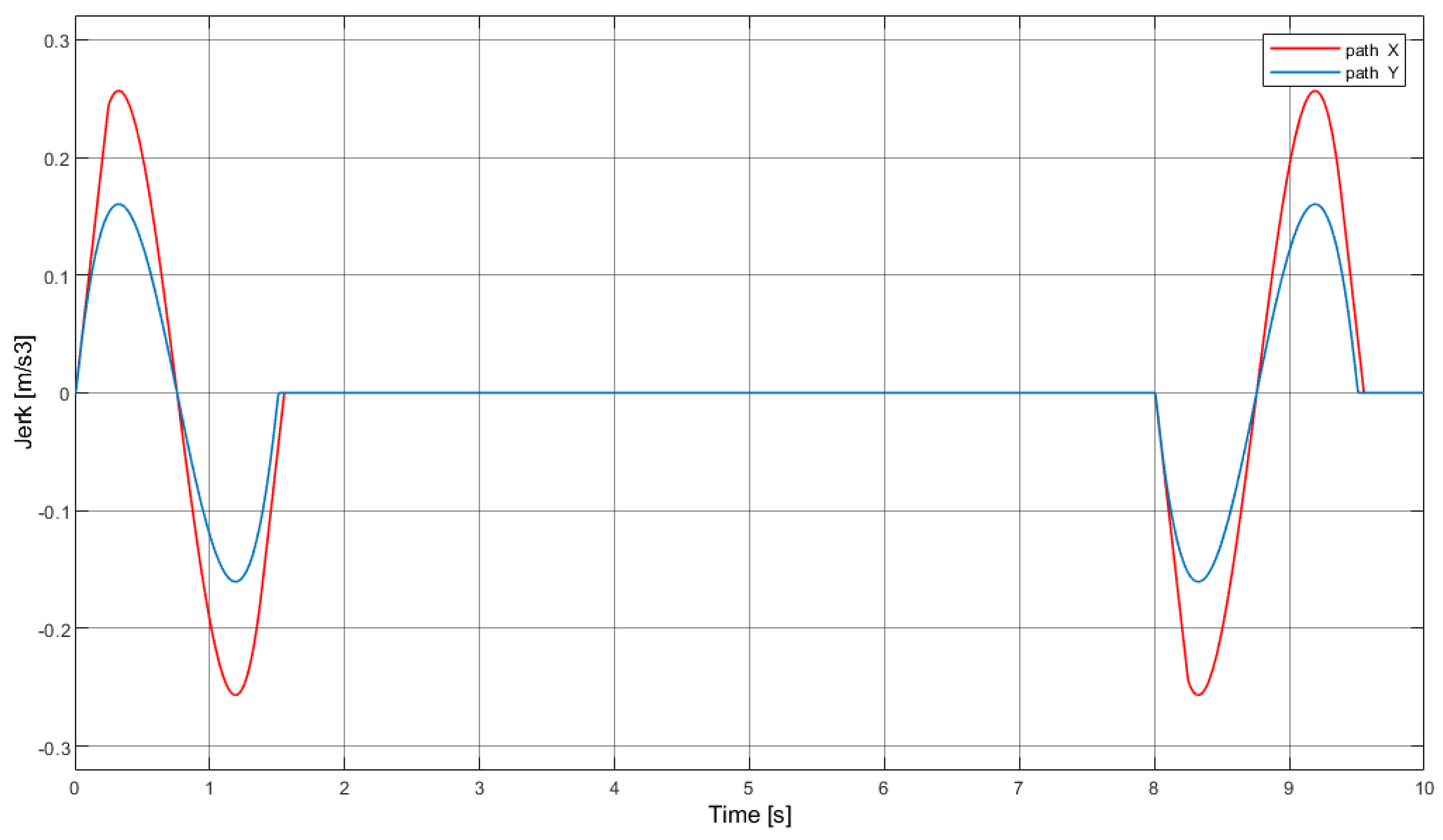
2.3. Trajectory Planning

The trajectory planning of a robot allows us to determine the continuous position paths that will guide the end-effector of the robot, either in the presence or absence of defined obstacles in its workspace. In this sense, trajectory planning seeks to determine continuous and smooth trajectories in position, speed, acceleration, and jerk for each active joint of the robot, guaranteeing their physical integrity [25].

To meet the expressed requirements of path continuity and smoothness, a 6-1-6 polynomial path can be adjusted [21]. This position path has a sixth-order polynomial in the acceleration and deceleration section, while the middle section guarantees constant speed with a first-order polynomial. The generic polynomial structure 6-1-6 is:

$$h_A\left(t\right)=\frac{v_{max}}{t_{ac}{}^5}{t}^6-\frac{3v_{max}}{t_{ac}{}^4}{t}^5+\frac{5v_{max}}{2t_{ac}{}^3}{t}^4+X_0$$

(5)

$$h_B\left(t\right)=v_{max}t+\frac{v_{max}{t}_{ac}}{2}+X_0$$

(6)

$$h_c\left(t\right)=-h_A\left(t\right)+v_{max}t+\left(tt-\frac{3v_{max}}{2}{t}_{ac}\right)v_{max}+2X_0$$

(7)

The values considered along each axis of the robot are:

• $h_A$, $h_B$, and $h_C$: positions reached during the sections of acceleration, constant speed, and deceleration, respectively.
• $v_{max}$: maximum speed that can be developed.
• $t_{ac}$: acceleration and deceleration time.
• $tt$: total time required to develop the whole trajectory.

In Figure 4, the graph of the trajectories 6-1-6 in the task space can be seen, which was used for the robot as positional references. In Figure 5, Figure 6 and Figure 7, the curves for speed, acceleration, and jerk are shown, which were derived from the position curve, showing that in all cases they were smooth paths that did not present discontinuities [21].

2.4. Controller Tuning

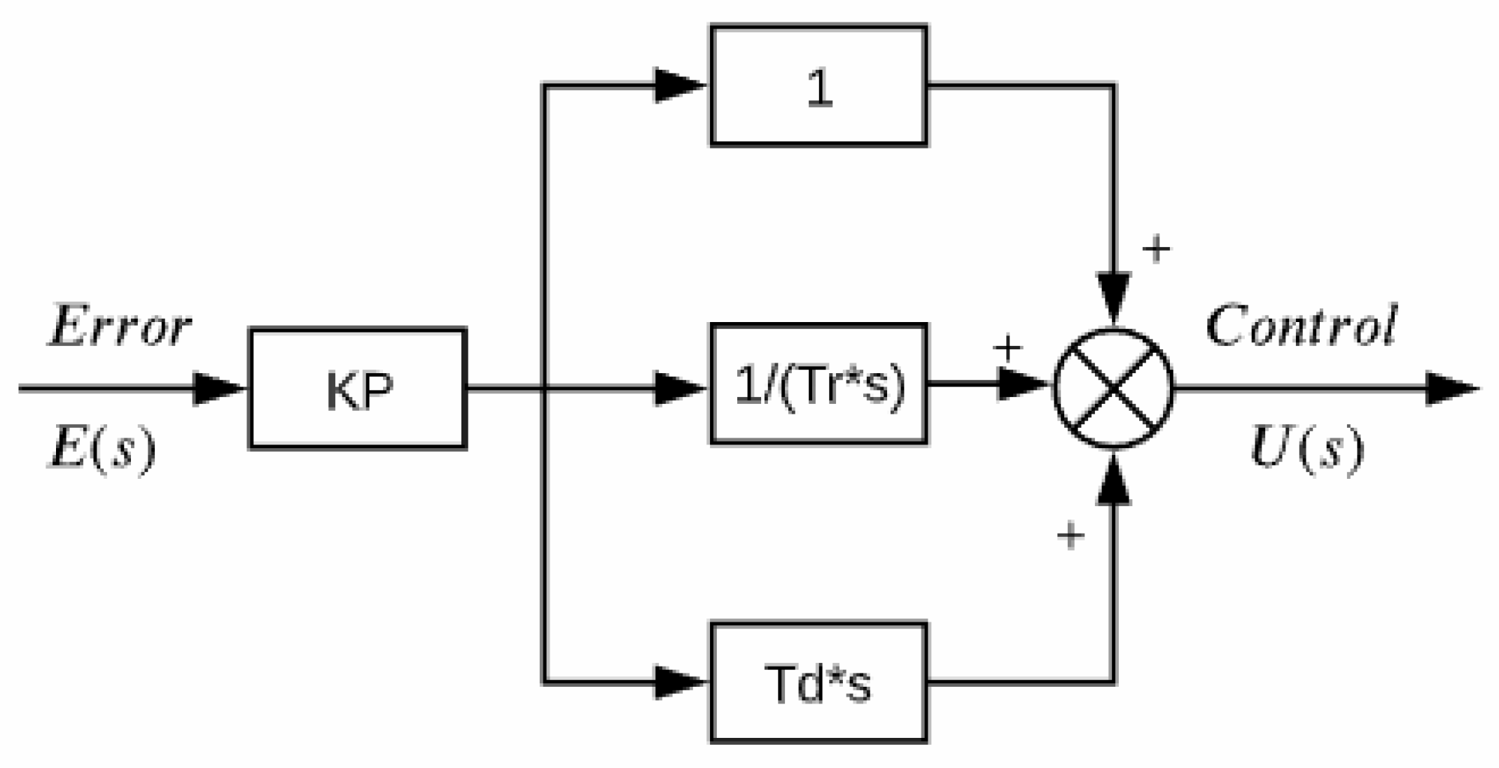
Based on the dynamic behavior of the system, various controller structures can be adopted for the implementation of the control block, among them PID controllers and fuzzy PID control, which were chosen for this work due to their advantages in tuning and robustness.

2.4.1. PID Control

One of the most used controllers in the industry is the proportional, integral, and derivative (PID) controller.

In Figure 8 the structure of a PID is shown, whose general equation is:

$$U\left(s\right)=\mathrm{KP}\left(1+\frac{1}{\mathrm{Tr}\ast \mathrm{s}}+\mathrm{Td}\ast \mathrm{s}\right)E\left(s\right)$$

(8)

where:

U(s): Control signal

KP: Proportional constant.

E(s): Error signal (difference between reference and controller response).

Tr: Adjustment constant for integral action.

Td: Adjustment constant for derivative action.

Based on the Ziegler–Nichols [13] tuning technique, the constants KP, Tr and Td are proposed as a function of the critical period (Pc) and the critical gain (Kc). For the controller structure shown in Equation (8), the PID constants are obtained from Equations (9)–(11):

KP = 0.6 × Kc

(9)

Tr = Pc/2

(10)

Td = Pc/8

(11)

Through the simulation, the critical force value was found in the upper cables, which allow for the balance of the robot in the center of the work plane, for which an approximate force of 2.7 N resulted. This value of the force will be considered as the operating point around which the control signal will act. The proposed control structure has a block that compensates for the forces of the effector’s weight, which in this case corresponds to forces of 2.7 N for each upper cable.

In order to generate an oscillation of the system, a force slightly greater than the force that stabilizes it is applied. In this case, a force of 3 N was applied to the upper cables, so that with the robot originally positioned in the center of the plane, oscillations were produced in the vertical axis, allowing the critical period (Pc) to be obtained for the calculation of the controller’s parameters. According to Figure 9, the period of oscillation was Pc = 4 s. In the first instance, a critical gain Kc = 1 was assumed, since it used forces very close to the forces that balance the robot in the center of the plane. This gain can be adjusted based on the response of the system.

The PID parameters shown in Equation (8), resulted in Kp = 0.6, Tr = 2, and Td = 0.5. These constants were configured in the two control blocks shown in the structure of Figure 3, which, including the gravitational forces compensation stage, remains as shown in Figure 10.

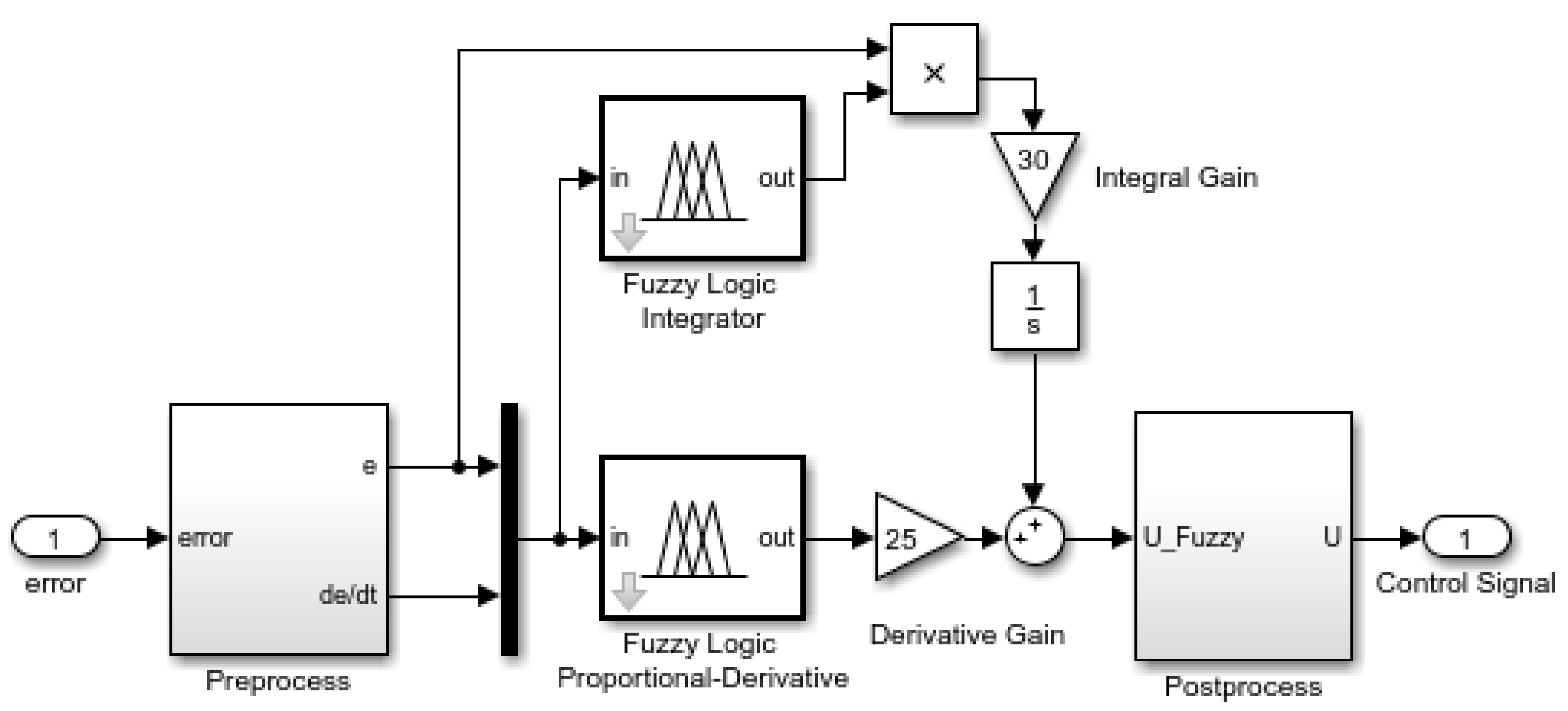
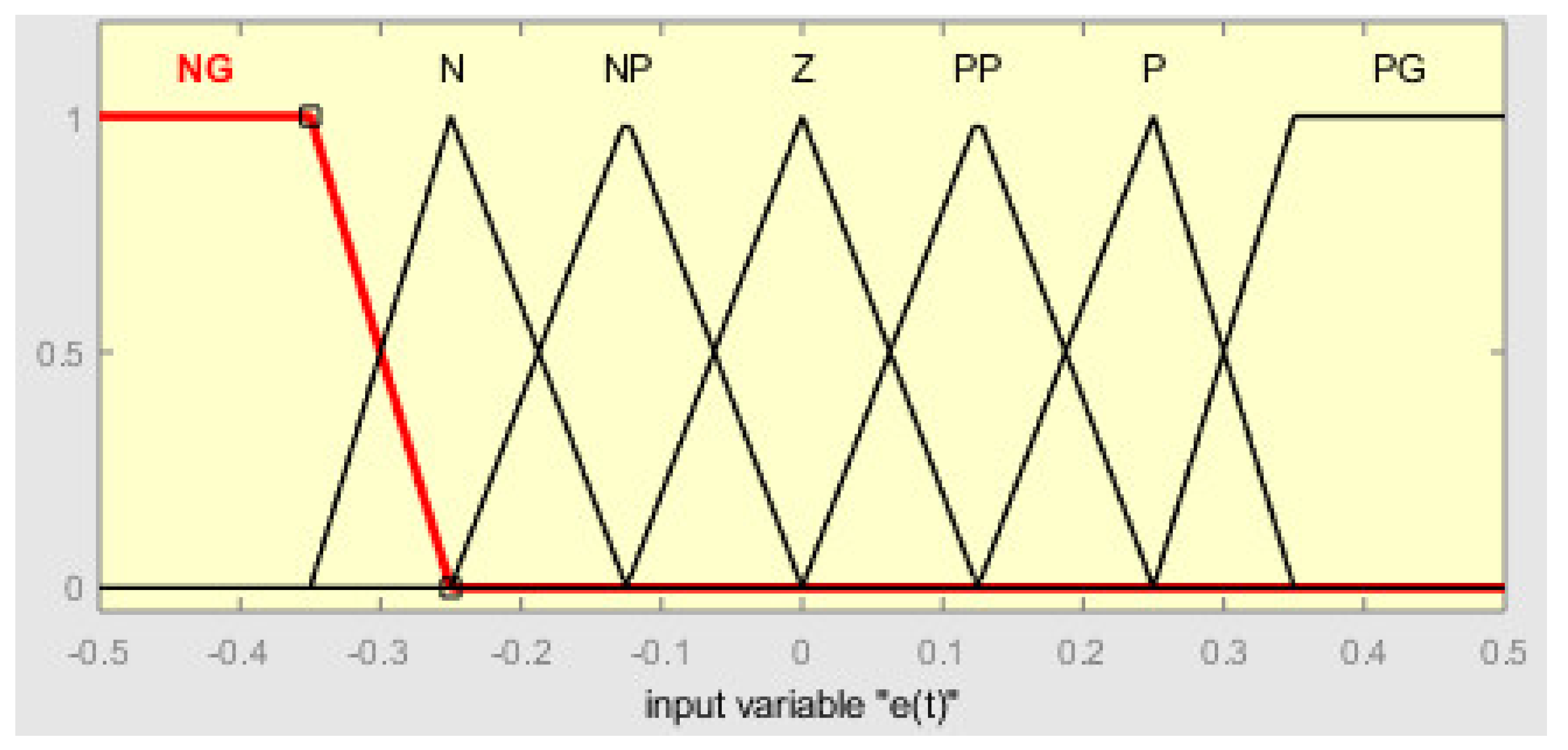
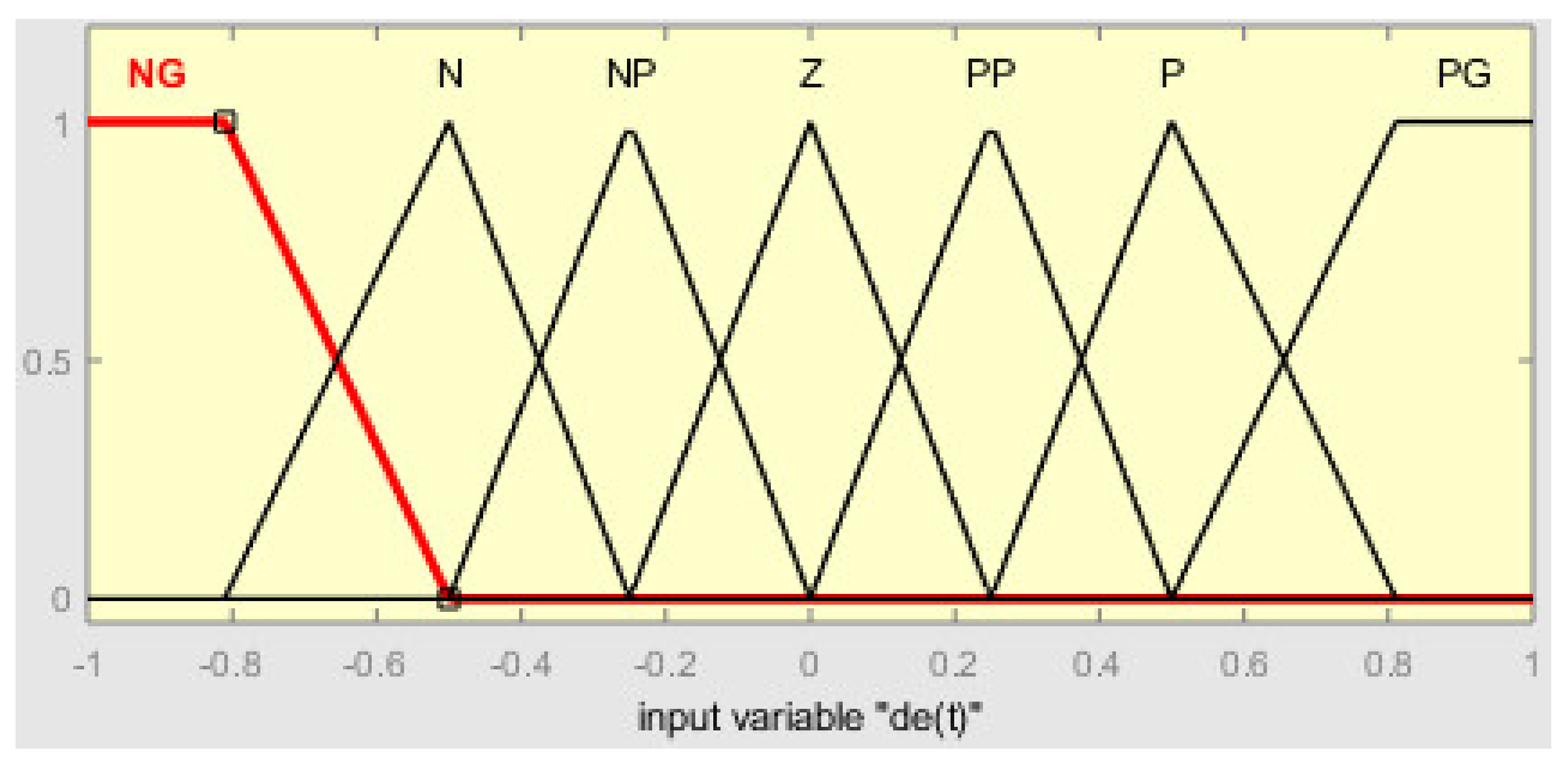
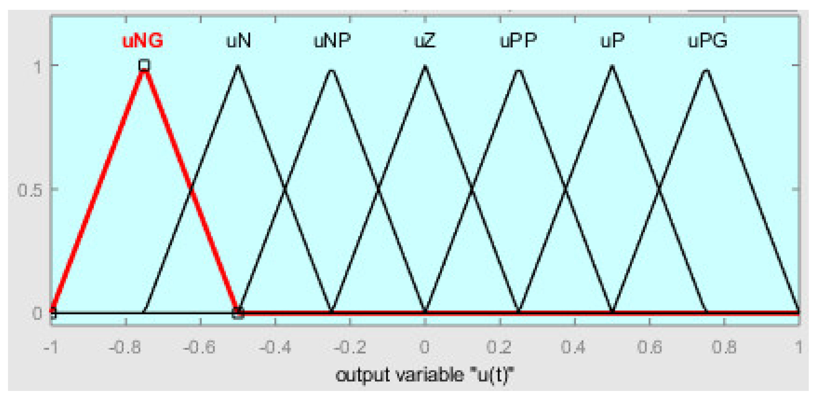
2.4.2. Fuzzy Control

The fuzzy controller is by nature a non-linear controller whose most relevant characteristics are:

∘

It does not require knowledge of the mathematical model of the plant to be controlled.

∘

The control output is generated by inference of the input signals based on the membership functions defined for each variable, establishing its form and respective universe of discourse.

∘

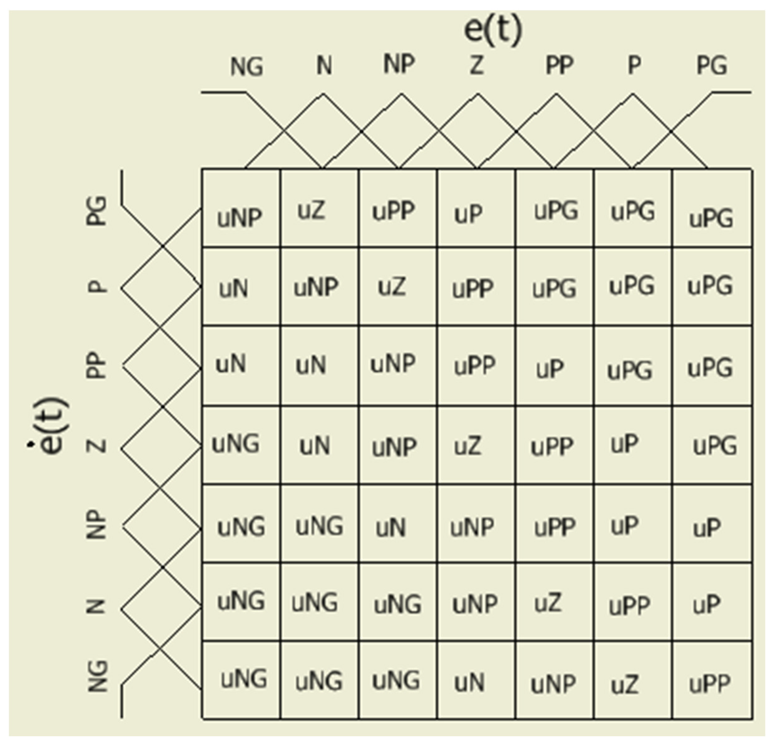
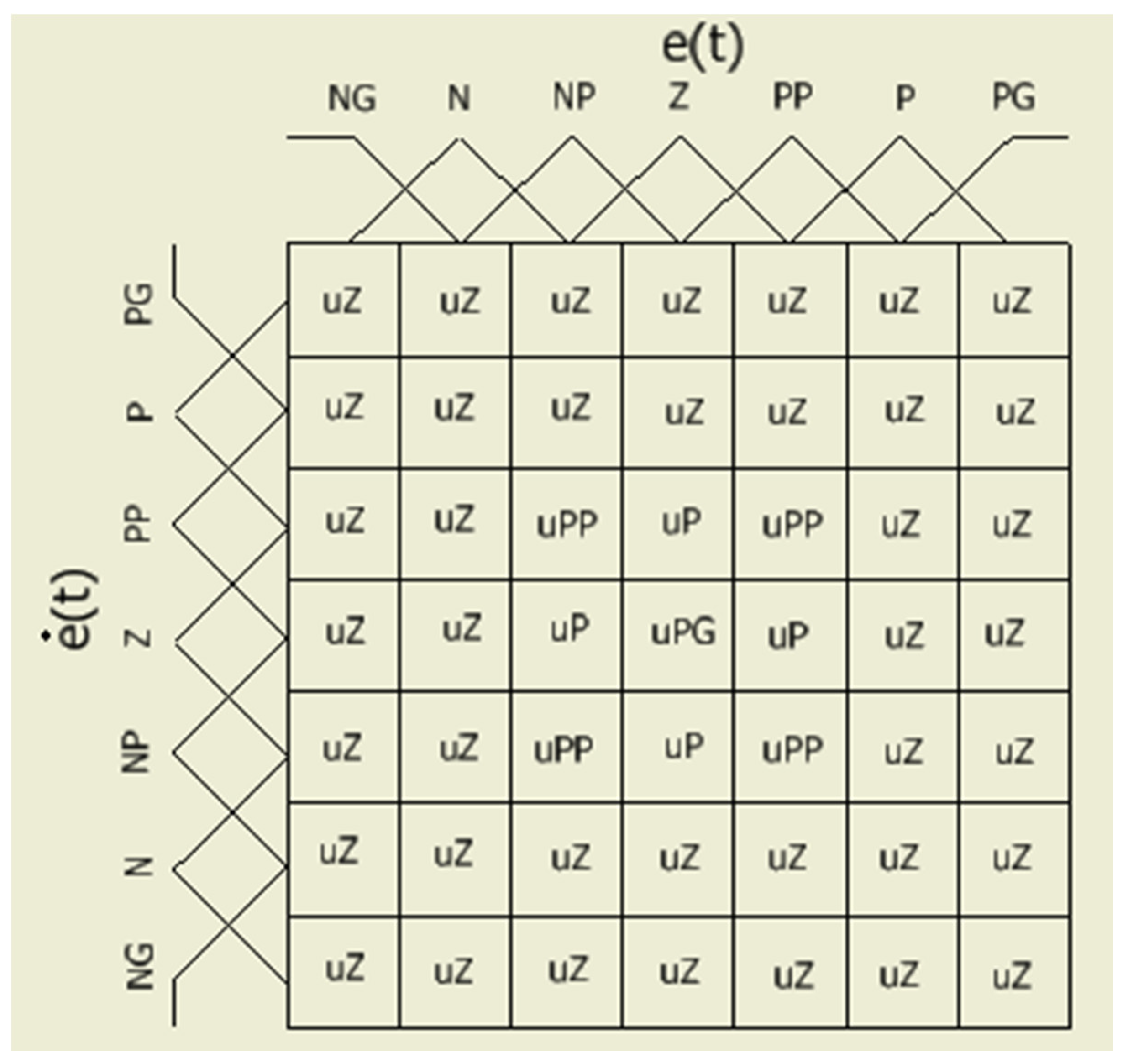
The inference is developed through a rules table of query and decision.

For fuzzy controller tuning, it is very important to define the universe of discourse of each membership function according to the knowledge of the system’s operation (operator experience).

A fuzzy logic controller can adopt the structure of a PID controller with the generation of output functions derived from PD action and an adaptation for the integrating signal, as can be seen in Figure 11.

An independent control structure was chosen for the proportional–derivative and the integral terms, which provided us the possibility of separately adjusting the incidence of each stage according to the response requirements that were presented in the fine-tuning process of the controller by modifying the gain value during each stage. This action replaces the effect of having to make multiple modifications in the universe of discourse of the variables.

For the control of a planar CDPR by means of a fuzzy PID controller, the error signals and their derivatives were considered as inputs to the controller. The selection of the rules and the number and form of the membership functions were based on expert knowledge acquired in the operation of a didactic planar CDPR belonging to Salesian Polytechnic University, as shown in Figure 12. The structure of the model shown in Figure 1, as well as its physical dimensions, were also based on this didactic CDPR. The inference process in the set of rules was of the Mamdani type [26].

The physical dimensions of the robot’s workspace described above were directly involved in the choice of the universe of discourse of the error variables. Additionally, with the intention of achieving a more effective action when the robot approached the desired position, it was decided to concentrate the membership functions in the universe of discourse between −0.5 m and 0.5 m, taking into account that if the error were greater it, would be captured by the lateral membership functions which have open trapezoidal characteristics. On the other hand, in the case of the universe of discourse for the signal of the derivative of the error, the maximum speed of movement of the robot was considered, which is 2 m/s in the end-effector. Therefore, using a similar criterion for the action of the membership functions that focused their action on when the robot approached the desired position, a universe of discourse ranging from −1 m/s to 1 m/s was defined.

Seven membership functions were considered for each input signal to the controller (error signal and derivative of the error), of which the intermediate five were triangular type and those at the ends were open-wing trapezoidal type, as shown in Figure 13 and Figure 14. These membership functions were distributed evenly throughout the universe of discourse and named: large negative (NG), negative (N), small negative (NP), zero (Z), small positive (PP), positive (P), and large positive (PG).

These seven membership functions were equidistant in distribution, with each corresponding to 14.2% of the universe of discourse. In the case of the error signal, each membership function was equivalent to approximately 14 cm, and in the case of the derivative of the error, it corresponded to 0.28 m/s. These ranges and the number of membership functions were considered acceptable as they generated control surfaces requiring a moderate amount of computation.

The control output was generated by the inference of seven triangular membership functions, as seen in Figure 15 [26,27]. These membership functions represent the characteristics of the control signal and were named: large negative control (uNG), negative control (uN), small negative control (uNP), zero control (uZ), small positive control (uPP), positive control (uP), and large positive control (uPG).

The choice of the triangular shape of the membership functions used for the inputs and output was intended to decrease the processing time, understanding that the generated control surfaces would not be physically smooth. It should be noted that the general context of the smooth motion of the robot was considered in the design of the trajectory planner.

The output signal of both the proportional–derivative stage and the integrating stage was derived from an inference process based on AND operations that had a total of 49 rules, whose details are shown in Figure 16 and Figure 17. Each rule was constructed based on expert knowledge of CDPR behavior, and some examples are explained:

• For the output of the proportional–derivative action when the error signal and the error derivative are close to zero, the rule can be stated as: IF e(t) is “Z” AND $\dot{e}\left(t\right)$ is “Z” THEN u(t) is “uZ.” The same situation for the output of the integrative action can be stated as: IF e(t) is “Z” AND $\dot{e}\left(t\right)$ is “Z” THEN u(t) is “uPG.” In this case, the idea is that the integrative action is in charge of outputting the required control signal that maintains the tracking error near zero.
• If a small positive error is now considered with a small negative error derivative, a small positive action would be required at the output of the proportional–derivative action and this rule can be stated as: IF e(t) is “PP” AND $\dot{e}\left(t\right)$ is “NP” THEN u(t) is “uPP.”
• If again, a small positive error is considered, but now a small positive error derivative is present, then the output of the proportional-derivative action must be reinforced, and this can be stated as: IF e(t) is “PP” AND $\dot{e}\left(t\right)$ is “PP” THEN u(t) is “uP.”

The defuzzification process of the Mamdani fuzzy inference system is based on the centroid calculation, where the defuzzified value x* for a fuzzy input is obtained by:

$$x^{*}=\frac{{{\displaystyle \int }}_a^{b}x\mu \left(x\right)dx}{{{\displaystyle \int }}_a^b\mu \left(x\right)dx}$$

(12)

where µ(x) is the fuzzified input, and [a,b] is the interval where the fuzzy set is defined [28].

Once the set of rules was implemented, the control surfaces obtained for each stage were observed, as shown in Figure 18 and Figure 19.

The structure and tuning of the fuzzy controller can be implemented in an equivalent way for the control of the X-axis and the Y-axis, according to the planar CDPR decoupled control system structure shown in Figure 3.

3. Results

The CDPR planar control system is shown in Figure 20, which includes a disturbance signal input that allows for the validation of the results of the controllers in the presence of any external signal that may deviate it from the objective position of the robot. The simulations were developed in MATLAB/Simulink using continuous-time mode, with fixed step size and an ode4 (Runge–Kutta) solver.

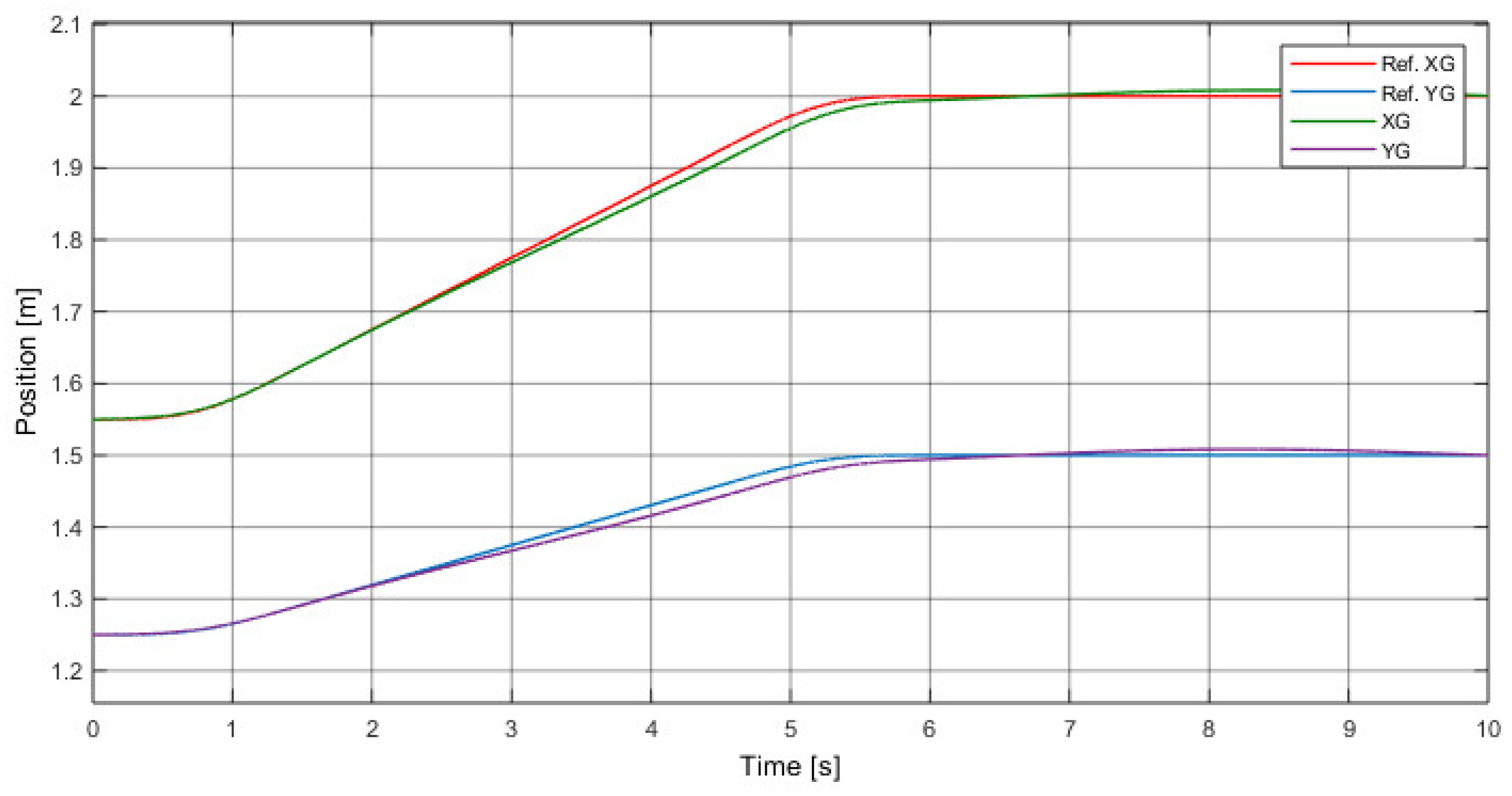
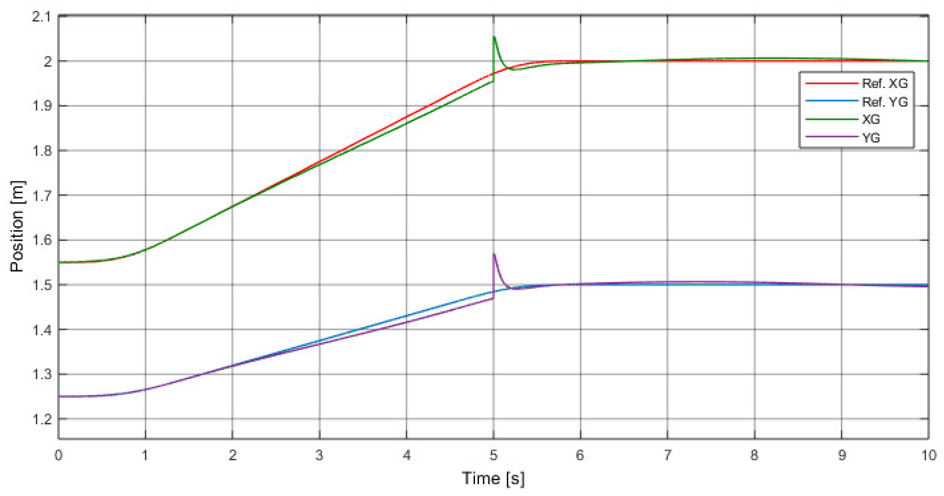
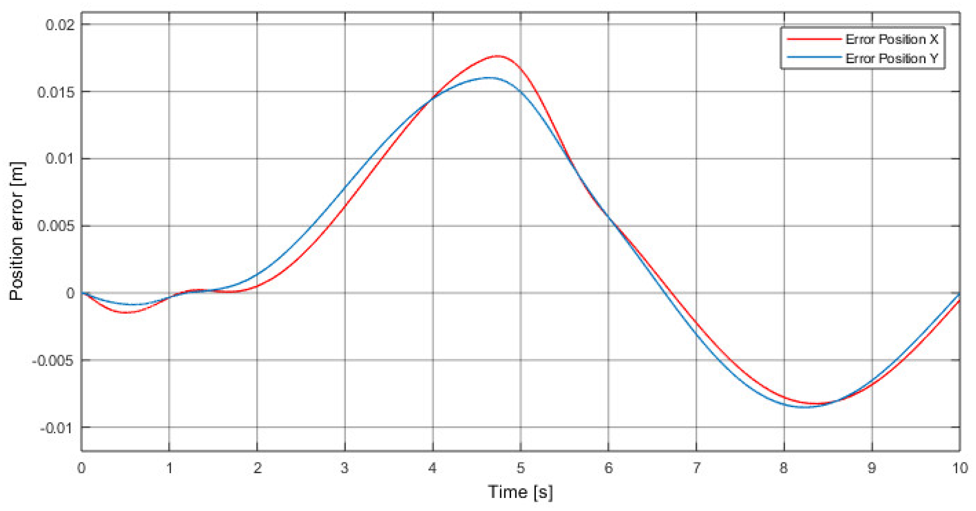
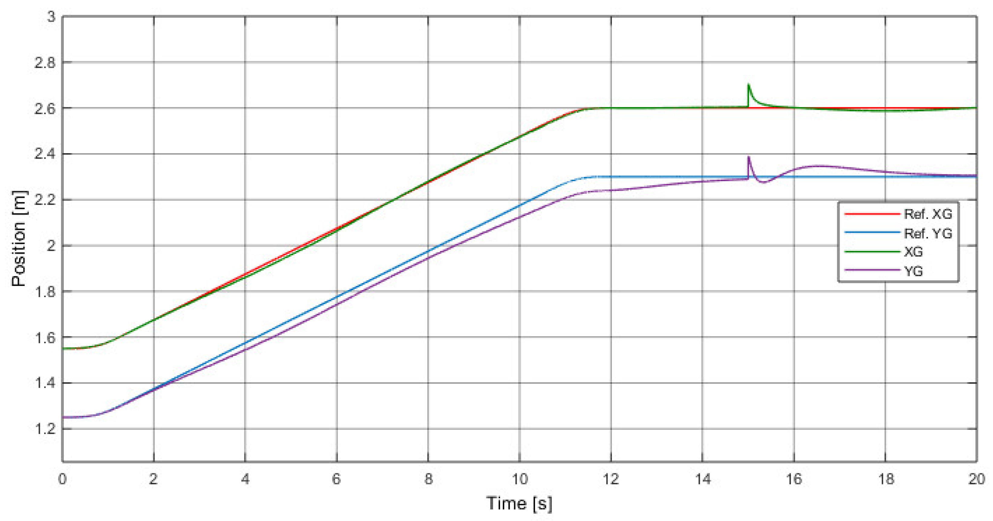
3.1. Simulation Results for a Control Structure Based on PID Controllers

The results of the simulations for the control structure of Figure 10 based on PID controllers are presented below.

The position in the X and Y axes of the end-effector of the robot is represented by XG and YG. The references generated by the trajectory planner are called Ref. XG and Ref. YG.

Figure 21 shows the robot’s positioning response in the absence of disturbance actions, while Figure 22 shows the results in the presence of 10 cm step disturbance actions in the position of each axis.

In Figure 21 and Figure 22, it can be seen that the robot followed the positional reference, establishing itself with relative precision, and was also capable of overcoming the disturbance present after 5 s of simulation.

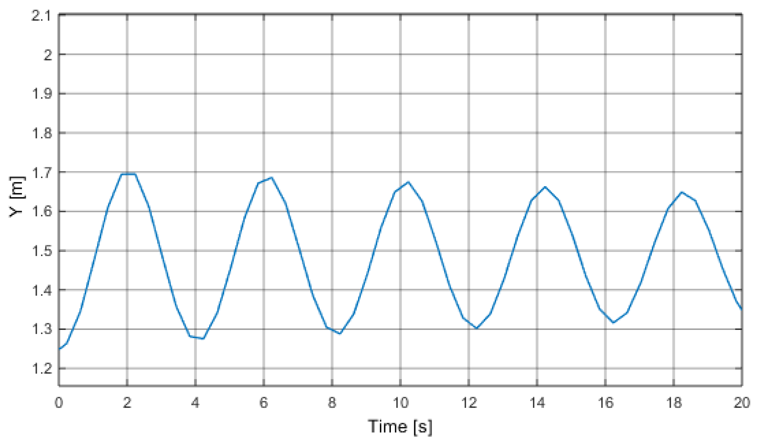
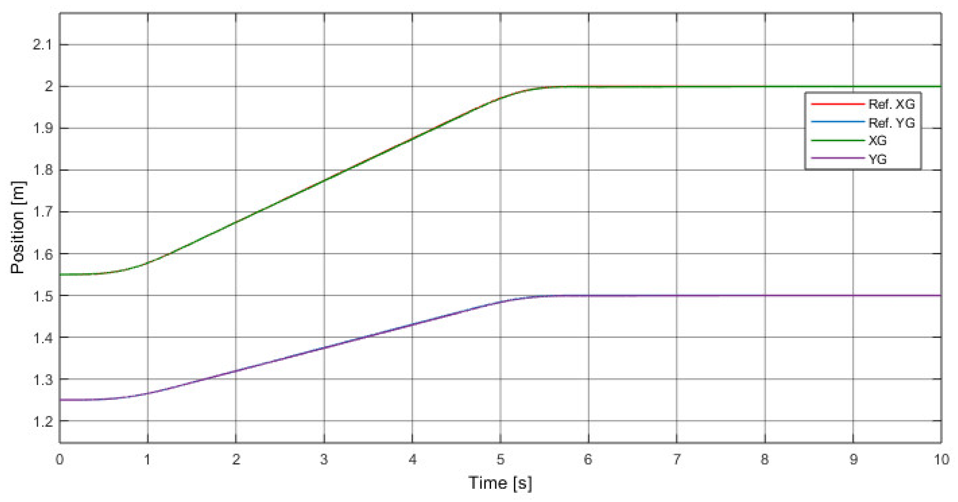
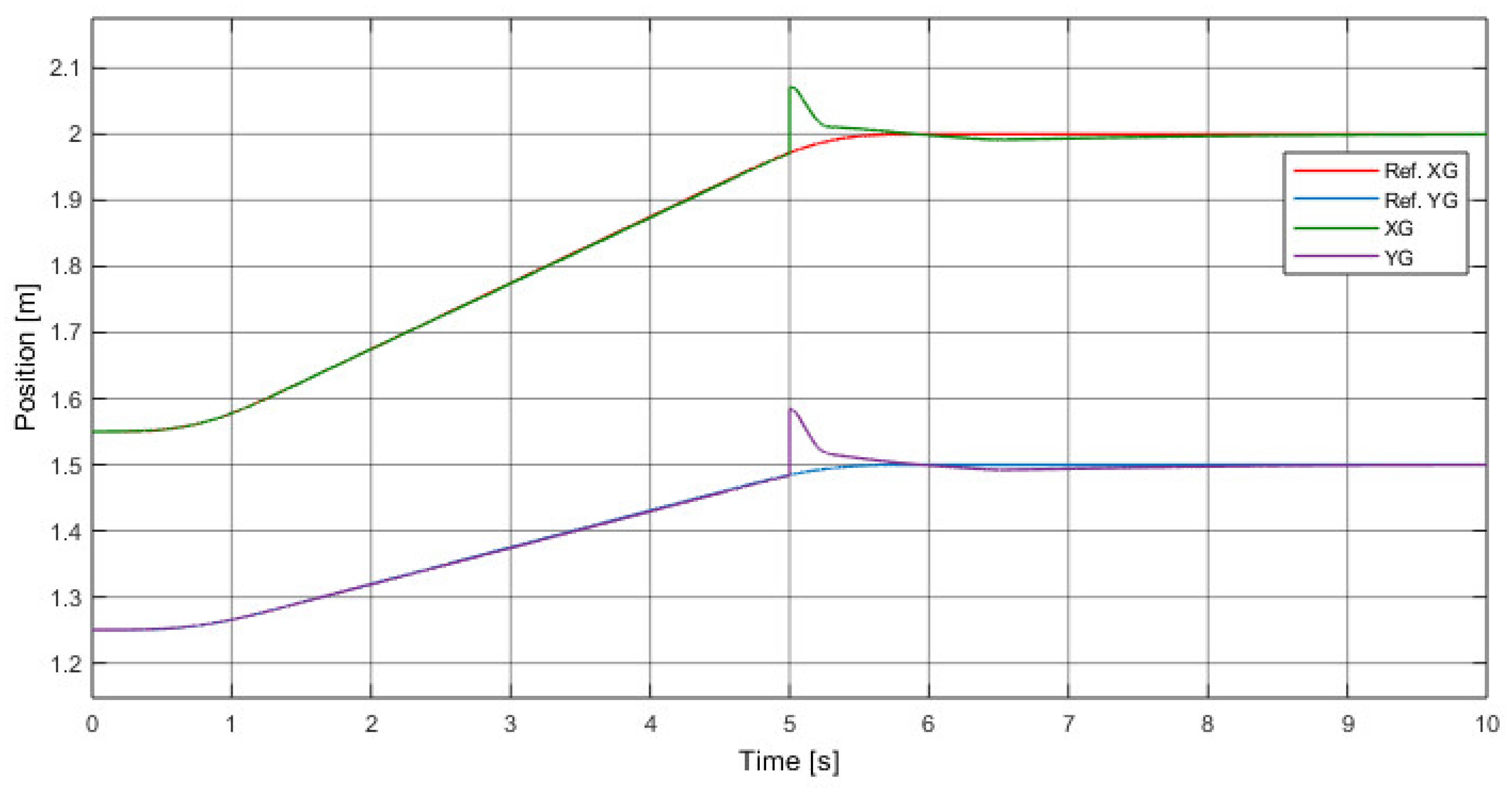
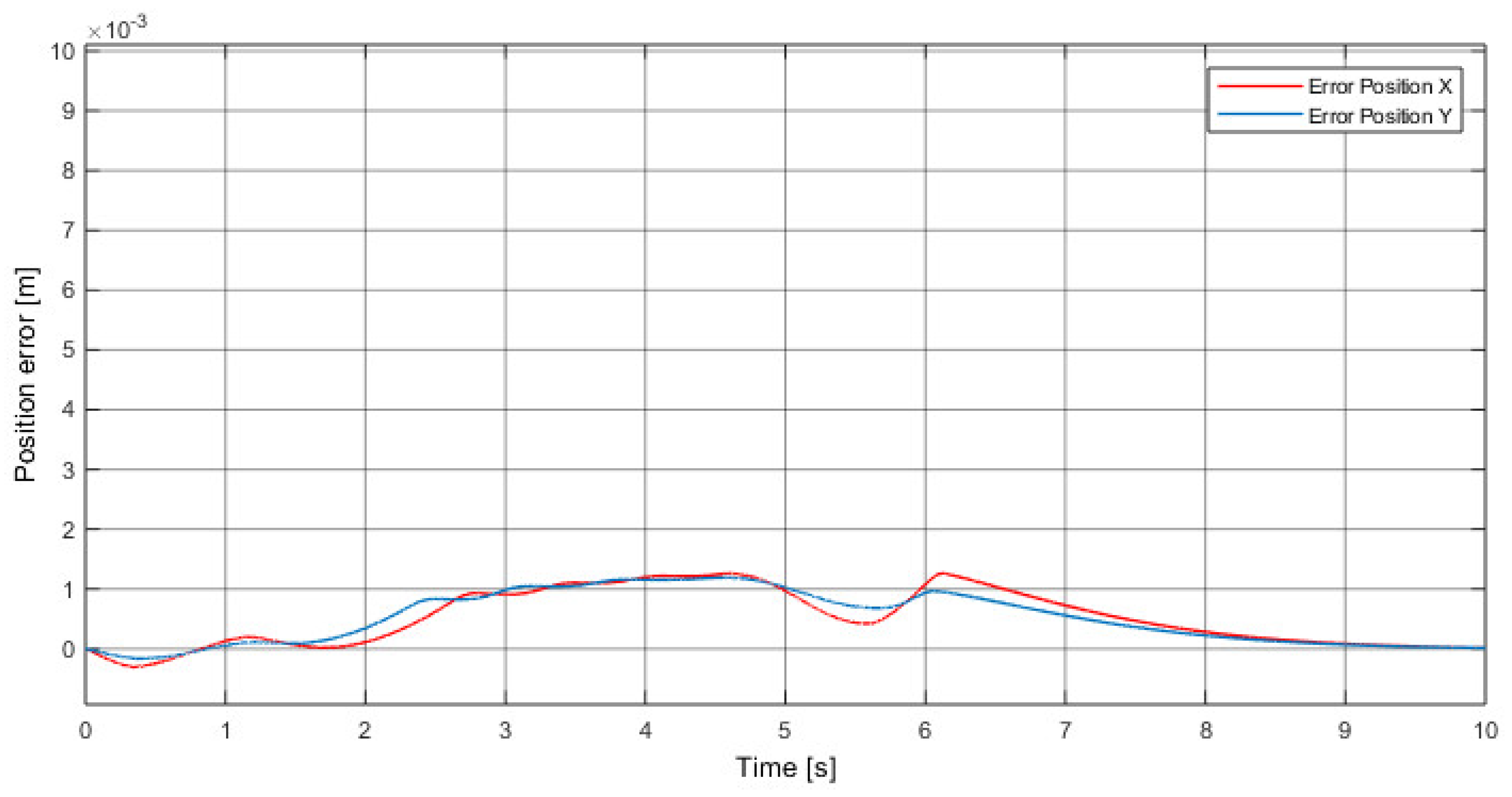
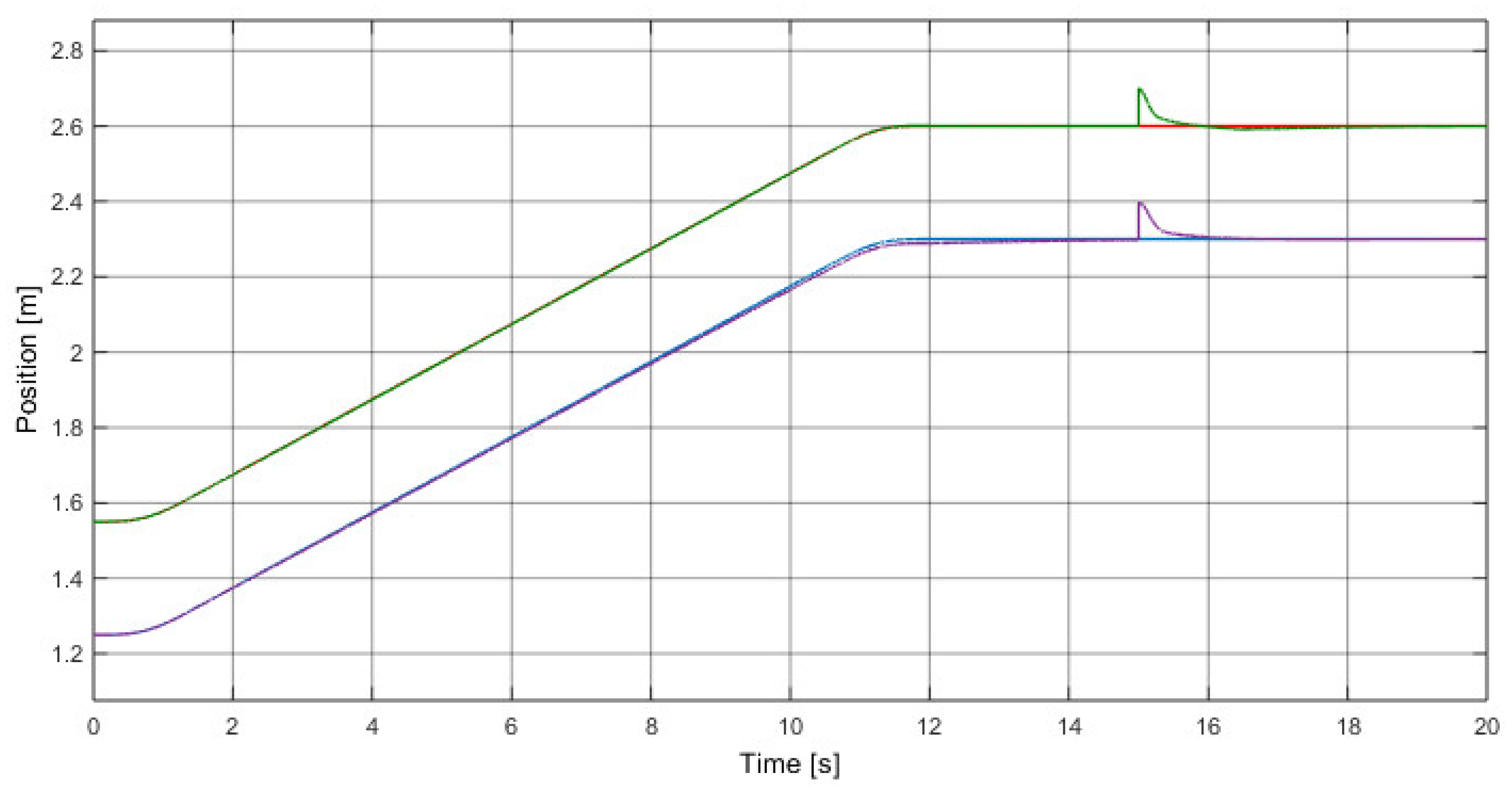
3.2. Simulation Results for Control Structure Based on Fuzzy-PID Controllers

The results of the simulations for the control structure of Figure 10 based on fuzzy PID controllers are presented below.

In Figure 23, the response of positioning and orientation of the robot can be observed in the absence of disturbance actions, while in Figure 24 the results are observed in the presence of 10 cm step disturbance actions in the position of each axis.

In a similar way to the case of control with a PID, it is observed in Figure 23 and Figure 24 that the robot followed the position reference, was established with better precision and was able to overcome the disturbance presented through 5 s of simulation. Although the disturbance rejection was no better than that of a classic PID, a lower tracking error was observed throughout the path. In order to compare the performances of both controllers, the cumulative quadratic error (CQE) between responses and their corresponding references was computed in MATLAB. For the test of the PID shown in Figure 21, the CQE was 0.41 for the response on the X-axis and 0.37 for the response on the Y-axis. The same index calculated for the response of the fuzzy PID shown in Figure 23 gave 0.0056 in the X-axis and 0.0058 in the Y-axis.

4. Discussion

According to the results, it was determined that the decoupled control structure proposed in this document, which considers the movements in the axes of the robot plane as independent, was effective when implemented with both classic and fuzzy PID controllers. During a combined movement on both axes, each controller was influenced by the signals generated because of the movement on the other axis. This influence is assumed as a disturbance that will be controlled by the controller. The effectiveness of the control depends on the distance between the end-effector and the center of the plane of movement, being lower as the end-effector moves away from the center.

The fuzzy PID controller had notably better performance compared to the classic PID, as shown previously with the calculated values of the CQE. These can be also observed in the error signals of the evolutions shown in Figure 21 and Figure 23, which are plotted in Figure 25 and Figure 26.

It is important to highlight that compensation for gravitational forces calculated in the center of the workspace was proposed. The non-linearity of the system restricted the performance of the controllers to an area close to this point of operation. Therefore, the workspace under the proposed control structure was affected. In this sense, a point more distant from the center of the robot [X, Y] = [2.6, 2.3] was explored, with the disturbing position signal acting after 15 s. Figure 27 and Figure 28 show the responses of the PID control system and the fuzzy PID, respectively, in which it can be seen that the PIDs did not present an adequate control action.

5. Conclusions

The results show that PID controllers with linear characteristics correctly control the non-linear mechanism under a decoupled structure for each axis of the end-effector. However, by having a defined operation point at the center of the robot, these controllers lose effectiveness at positioning the robot at extreme points of the work plane, reducing the effective working space of the robot.

It was observed that the fuzzy PID controllers, having non-linear characteristics, controlled the non-linear mechanism with greater accuracy, and presented smaller error signals than those of the control case based on classic PID controllers. Additionally, it was shown that fuzzy PID controllers presented an adequate level of performance in extreme positions of the robot, allowing us to effectively take advantage of a wider workspace with respect to the case of the PID controllers.

As was shown, when analyzing the behavior of the error signal developed by the control system for each case, the control system based on fuzzy PID presented better results in terms of the amplitude of the error and the stabilization time.

The decoupled control structure proposed for each axis of the planar CDPR has proven to be effective even when it was experimented upon using trajectories of simultaneous movement between the two axes.

Future work should include an experimental test of the proposed CDPR method shown in Figure 12. Also, future work should extend the application of this structure to the case of a spatial CDPR in which decoupled movements are assumed for the three axes.

References

1. Sun, H.; Tang, X.; Cui, Z.; Hou, S. Dynamic Response of Spatial Flexible Structures Subjected to Controllable Force Based on Cable-Driven Parallel Robots. IEEE/ASME Trans. Mechatron. 2020, 25, 2801–2811. [Google Scholar] [CrossRef]
2. Zhang, B.; Shang, W.; Cong, S.; Li, Z. Coordinated Dynamic Control in the Task Space for Redundantly Actuated Cable-Driven Parallel Robots. IEEE/ASME Trans. Mechatron. 2020. [Google Scholar] [CrossRef]
3. Picard, E.; Caro, S.; Franck, P.; Claveau, F. Control Solution for a Cable-Driven Parallel Robot with Highly Variable Payload. Mech. Robot. Conf. 2018, 5B, 26–29. [Google Scholar]
4. Tho, T.P.; Thinh, N.T. Using a Cable-Driven Parallel Robot with Applications in 3D Concrete Printing. Appl. Sci. 2021, 11, 563. [Google Scholar] [CrossRef]
5. Gosselin, C. Cable-driven parallel mechanisms: State of the art and perspectives. Mech. Eng. Rev. 2014, 1, DSM0004. [Google Scholar] [CrossRef] [Green Version]
6. Merlet, J.; Papegay, Y.; Gasc, N. The Prince’s tears, a large cable-driven parallel robot for an artistic exhibition. In Proceedings of the IEEE International Conference on Robotics and Automation, Paris, France, 31 May–31 August 2020; pp. 10378–10383. [Google Scholar]
7. Jung, J. Workspace and Stiffness Analysis of 3D Printing Cable-Driven Parallel Robot with a Retractable Beam-Type End-Effector. Robotics 2020, 9, 65. [Google Scholar] [CrossRef]
8. Chen, Y.; Shao, L.; Liu, S.; Zhang, Y.; Wang, H. Adaptative Fuzzy Control for a Class of Nonlinear Time-Delay Systems. In Proceedings of the IEEE Data Driven Control Learn. Syst. Conf. (DDCLS), Cairo, Egypt, 14–16 December 2020; pp. 1125–1130. [Google Scholar]
9. Ma, X.-J.; Sun, Z.-Q.; He, Y.-T. Analysis and design of fuzzy controller and fuzzy observer. IEEE Trans. Fuzzy Syst. 1998, 6, 41–51. [Google Scholar]
10. Erenoglu, I.; Eksin, I.; Yesil, E.; Guzelkaya, M. An Intelligent Hybrid Fuzzy PID Controller. In Proceedings of the 20th European Conference on Modelling and Simulation, Bonn, Germany, 28–31 May 2006; pp. 1–5. [Google Scholar] [CrossRef] [Green Version]
11. Dewantoro, G.; Kuo, Y. Robust speed-controlled permeant magnet synchronous motor drive using fuzzy logic controller. In Proceedings of the IEEE International Conference on Fuzzy Systems (FUZZ-IEEE), Taipei, Taiwan, 27–30 June 2011; pp. 884–888. [Google Scholar]
12. Yunong, Y.; Ha, H.M.; Kim, Y.K.; Lee, J. Balancing and driving Control of a ball robot using fuzzy control. In Proceedings of the International Conference on Ubiquitous Robots and Ambient Intelligence (URAI), Goyangi, Korea, 28–30 October 2015; pp. 492–494. [Google Scholar]
13. Zabbah, I.; Foolad, S.; Chaharaqran, B.; Mazlooman, R. Design and making the intelligence assistant robot and controlling it by the fuzzy procedure. In Proceedings of the International Conference on Electronics, Computer and Computation (ICECCO), Ankara, Turkey, 7–9 November 2013; pp. 168–171. [Google Scholar]
14. Sheikhalr, A.; Fakharian, A.; Adhami, A. Fuzzy adaptative control of omni-directional mobile robot. In Proceedings of the 13th Iranian Conference on Fuzzy Systems (IFSC), Qazvin, Iran, 27–29 August 2013; pp. 1–4. [Google Scholar]
15. Ziegler, J.G.; Nichols, N.B. Optimum settings for automatic controllers. Trans. ASME 1942, 64, 759–765. [Google Scholar] [CrossRef]
16. Li, J.; Li, Y. Dynamic analysis and PID control for a quadrotor. In Proceedings of the IEEE International Conference on Mechatronics and Automation, Beijing, China, 7–11 August 2011; pp. 573–578. [Google Scholar]
17. Kelly, R. A tuning procedure for stable PID control of robot manipulators. Robotica 1995, 13, 141–148. [Google Scholar] [CrossRef]
18. Cervantes, I.; Alvarez, J. On the PID tracking control of robot manipulators. Syst. Control Lett. 2001, 42, 37–46. [Google Scholar] [CrossRef]
19. Lumelsky, V. Effect of kinematics on motion planning for planar robot arms moving amidst unknown obstacles. IEEE J. Robot. Autom. 1987, 3, 207–223. [Google Scholar] [CrossRef]
20. Kim, J.; Jin, M.; Park, S.; Chung, S.; Hwang, M. Task Space Trajectory Planning for Robot Manipulators to Follow 3-D Curved Contours. Electronics 2020, 9, 1424. [Google Scholar] [CrossRef]
21. Barroso, A.; Saltaren, R.; Portilla, G.; Cely, J.; Carpio, M. Smooth Path Planner for Dynamic Simulators Based on Cable-Driven Parallel Robots. In Proceedings of the International Conference on Smart Systems and Technologies (SST), Osijek, Croatia, 10–12 December 2018; pp. 145–150. [Google Scholar]
22. Max, H. Cable Structures, 1st ed.; The MIT Press: Cambridge, MA, USA, 1981; pp. 2–255. [Google Scholar]
23. Taghirad, H. Parallel Robots: Mechanics and Control, 1st ed.; CRC Press: Boca Raton, FL, USA, 2013; pp. 1–533. [Google Scholar]
24. Merlet, J. Parallel Robots, 2nd ed.; Springer: Paris, France, 2006; pp. 4–320. [Google Scholar]
25. Macfarlane, S.; Elizabeth, A. Jerk-Bounded Manipulator Trajectory Planning: Design for Real-Time Applications. Trans. Robot. Autom. 2003, 19, 42–51. [Google Scholar] [CrossRef] [Green Version]
26. Kaur, A.; Kaur, A. Comparison of Mamdani-Type and Sugeno-Type Fuzzy Inference Systems for Air Conditioning System. Int. J. Soft Comput. Eng. (IJSCE) 2012, 2, 323–325. [Google Scholar]
27. Carpio, M.; Orozco, W.; Betancur, M. Design and Simulation of a Fuzzy Controller for Vertical Take off and Landing (VTOL) Systems. In Proceedings of the International Autumn Meeting on Power, Electronics and Computing (ROPEC), Ixtapa, Mexico, 9–16 November 2016. [Google Scholar]
28. Ponce, P. Artificial Intelligence with Applications to Engineering, 1st ed.; Alfaomega: Mexico City, Mexico, 2010; pp. 72–75. [Google Scholar]
Figure 1. Planar CDPR structure.
Electronics 10 00745 g001
Figure 2. Topology of position control in task space.
Electronics 10 00745 g002
Figure 3. Control structure for the positioning of a planar CDPR.
Electronics 10 00745 g003
Figure 4. Trajectory for position using 6-1-6 polynomials for the planar CDPR.
Electronics 10 00745 g004
Figure 5. Trajectory for speed using 6-1-6 polynomials for the planar CDPR.
Electronics 10 00745 g005
Figure 6. Trajectory for acceleration using 6-1-6 polynomials for the planar CDPR.
Electronics 10 00745 g006
Figure 7. Trajectory for jerk using 6-1-6 polynomials for the planar CDPR.
Electronics 10 00745 g007
Figure 8. General structure of a PID controller.
Electronics 10 00745 g008
Figure 9. Oscillation response of the robot in the presence of 3 N forces in the upper cables.
Electronics 10 00745 g009
Figure 10. Structure of a decoupled control system for a planar CDPR.
Electronics 10 00745 g010
Figure 11. Structure of a fuzzy PID controller.
Electronics 10 00745 g011
Figure 12. Planar CDPR assembled in the labs of Salesian Polytechnic University in Ecuador.
Electronics 10 00745 g012
Figure 13. Membership functions and universe of discourse of the error input signal.
Electronics 10 00745 g013
Figure 14. Membership functions and universe of discourse of the error derivative input signal.
Electronics 10 00745 g014
Figure 15. Membership functions and universe of discourse of the control output signal.
Electronics 10 00745 g015
Figure 16. Matrix of rules for the proportional–derivative action.
Electronics 10 00745 g016
Figure 17. Matrix of rules for the integrative action.
Electronics 10 00745 g017
Figure 18. Control surface of the proportional-derivative action.
Electronics 10 00745 g018
Figure 19. Control surface of the integrative action.
Electronics 10 00745 g019
Figure 20. Control system of a planar CDPR.
Electronics 10 00745 g020
Figure 21. Planar CDPR positioning response of a PID controller.
Electronics 10 00745 g021
Figure 22. Positioning response of the planar CDPR in the presence of disturbance of a PID controller.
Electronics 10 00745 g022
Figure 23. Planar CDPR positioning response of a fuzzy PID controller.
Electronics 10 00745 g023
Figure 24. Positioning response of the planar CDPR in the presence of disturbance of a fuzzy PID controller.
Electronics 10 00745 g024
Figure 25. Error signal developed during robot movement under the action of a PID controller.
Electronics 10 00745 g025
Figure 26. Error signal developed during robot movement under the action of a fuzzy PID controller.
Electronics 10 00745 g026
Figure 27. Positioning response of the planar CDPR (away from the center) with disturbance at 15 s of simulation, with a PID controller.
Electronics 10 00745 g027
Figure 28. Positioning response of the planar CDPR (away from the center) with disturbance at 15 s of simulation, with a fuzzy PID controller.
Electronics 10 00745 g028
Publisher’s Note: MDPI stays neutral with regard to jurisdictional claims in published maps and institutional affiliations.