Article

Network Intelligent Control and Traffic Optimization Based on SDN and Artificial Intelligence

1
School of Economics and Management, Beijing University of Posts and Telecommunications, Beijing 100087, China
2
China United Network Telecommunications Corporation, Beijing 100048, China
*
Author to whom correspondence should be addressed.
Electronics 2021, 10(6), 700; https://doi.org/10.3390/electronics10060700
Submission received: 3 February 2021 / Revised: 7 March 2021 / Accepted: 15 March 2021 / Published: 16 March 2021
(This article belongs to the Special Issue New Trends in SDN/NFV Architectures and Routing Solutions)

Abstract

:
For telecom operators, it is of great significance to employ artificial intelligence (AI) and big data technology in a software-defined network (SDN) in order to achieve intelligent network control, traffic management and optimization. This paper proposes a solution for intelligent work control and traffic optimization. This paper is mainly focused on SDN-based network traffic algorithm optimization and experimental verification. In this paper, we design a network control mechanism for network intelligent control as well as solutions for traffic optimization based on SDN and artificial intelligence. We analyze operators’ network requirements (e.g., the carrying of the 5th generation mobile network (5G) service, multi-protocol label switching virtual private networks optimization, cloudification of services and the IP backbone network). Then, we propose an intelligent network control architecture based on SDN and artificial intelligence. The proposed architecture consists of three modules, including a network status collection/perception module, an AI intelligent analysis module and an SDN controller module. Moreover, this paper also analyzes the objects of traffic optimization as well as routing calculation algorithms (e.g., the greedy algorithm, the top-k-shortest paths (KSP) algorithm) and routing optimization algorithms (e.g., particle swarm optimization, simulated annealing and genetic algorithms). In addition, we also put forward three optimization algorithms for the operator’s network, namely, network congestion control and prevention algorithms, resource preemption algorithms and balance of the entire network traffic algorithms. Then, we propose optimization algorithms for the above three objectives of operator network optimization, respectively. Finally, we conduct large-scale experiments to verify the effectiveness of the control mechanism and algorithms. The experimental results demonstrate that the use of SDN and artificial intelligence in operator networks can realize network intelligent control and traffic optimization more intelligently.

1. Introduction

Network intelligent control has always been the goal pursued by operators. However, the optimization of the entire network traffic is a difficult problem, and it is also an urgent problem to be solved. Network intelligent control can improve network competitiveness. In addition, it can also improve network resource utilization and save costs [1,2]. Before the advent of SDN (software-defined networking), the network was distributed, whilst most of the existing methods could not achieve optimization of the entire network traffic, especially large operator networks. The main problems were as follows: (1) network planning and deployment were complicated, network paths were calculated in a distributed manner without a global perspective, and network traffic was poorly visualized; (2) the bandwidth utilization rate was low; it is difficult to achieve the optimal bandwidth utilization rate, and hence it is difficult for the network to respond to changes in network traffic in real time; (3) operation and maintenance is complex [3,4,5].
The basic idea of SDN is to separate the control plane of the network from the forwarding plane [6,7]. The logically centralized control plane can flexibly schedule network resources; in addition, the flexible interface can support the opening of network capabilities and the programming of the network control [8,9]. SDN can control packet forwarding flexibly, while SDN can also enable network control and strategies to be conveniently loaded on the forwarding device. This empowers the network to be more intelligent and flexible. SDN technology provides new ideas for operators’ network equipment reconfiguration and networking architecture [10,11] (e.g., separation of control and forwarding, virtualization, capability opening, dynamic reconfiguration, centralized management and control), which solve the problem of poor network reliability, low and unbalanced resource utilization rate, high operation and maintenance costs and other issues [12,13,14].
Artificial intelligence (AI) mainly plays the role of a “predictor” in network control and traffic optimization. AI algorithms empower data predictions to be more accurate, and AI algorithms make the network have cognitive capabilities and intelligent output capabilities. [15] Compared with traditional networks, networks with AI technology will not rely too much on human experience, and AI will assist network control and optimization through accurate data analysis and continuously optimized algorithms, thereby improving network resource utilization [16,17,18].
Traffic optimization and scheduling requires in-depth perception and precise control of services, users and network conditions, as well as unified management and analysis of network resources to form overall traffic optimization and scheduling strategies [19]. Traffic optimization and scheduling strategies mainly include the realization of the unified allocation and management of address resources, localized intelligent caching, traffic guidance and transmission, and coordinated allocation and the adjustment of IP layer link resources [20].
Through the detailed network information collected by the SDN controller, AI technology can actively predict the traffic carried by the link based on historical massive traffic data, and then AI can dynamically adjust traffic according to the link status (e.g., bandwidth, usage rate, reliability, cost, etc.) [21,22]. Therefore, network intelligent control and traffic optimization can be realized based on SDN and AI, and paths of different priority service traffic can be scheduled real-timely; in this way, it is possible to avoid local congestion and improve network quality and network utilization of the entire network.
In recent years, some scholars have introduced artificial intelligence algorithms into network path algorithms. Network path algorithms, which are based on neural networks, genetic algorithms (GA) and particle swarm optimization (PSO), have been designed. However, existing algorithms only consider one or several Quality of Service (QoS) path parameters, ignoring network resource consumption and allocation. These algorithms cannot effectively utilize and rationally allocate network resources, and both genetic algorithms and particle swarm optimization algorithms have their own shortcomings. They cannot meet the requirements of future networks for traffic optimization.
This paper proposes a solution for intelligent work control and traffic optimization. This paper is mainly focused on SDN-based network traffic algorithm optimization and experimental verification. The rest of this paper is organized as follows. Section 2 analyzes the scenarios and requirements of network intelligent control and traffic optimization. Section 3 proposes an architecture of intelligent work control. Section 4 provides a method and solution of traffic optimization. Section 5 gives the experimental validation results of the traffic optimization. Section 6 gives conclusions of the whole paper.

2. Scenarios and Requirements

2.1. The Carrying of 5G Services

The features of 5G technology (e.g., large bandwidth, low latency and massive connection) put forward higher requirements for mobile bearer networks. The 5G network needs to be able to perceive changes in service traffic trends, predict traffic, notify operation and maintenance personnel in advance to deal with them and prevent future service growth from causing local congestion and service damage [23]. These require the introduction of SDN and artificial intelligence technology which can intelligently predict traffic trends in the current network and optimize the traffic to make sure that traffic congestion will not affect the 5G service experience.
When the traffic of network link exceeds the set threshold, the traffic on the link needs to be optimized and adjusted in time to other spare links. If the traffic does not have detour conditions, it is necessary to limit the low-priority service traffic at the ingress to reduce the congested link bandwidth and always guarantee the service level agreement (SLA) quality of 5G high-priority services [24].

2.2. MPLS Network

With the development of various types of converged services, the network is required to provide a unified bearer of fixed network services and mobile network services, such as home broadband, government and enterprise dedicated lines and mobile base stations. Additionally, the entire network merges the metropolitan area network, the backbone network and the access network into one Multi-Protocol Label Switching (MPLS) domain. The entire network carries multiple services based on a unified IP/MPLS technology, which means that one network is allowed to carry all services. In this scenario, the network is required to realize flexible scheduling and the optimization of different flows according to service requirements and user priorities so as to improve network utilization efficiency and guarantee the experience of various services.

2.3. Cloudification of Services and IP Backbone Network

In recent years, the cloudification of services has brought greater convenience to users and content providers, but it has also brought difficulties to the prediction of service traffic models. This leads to a large deviation between actual network utilization and network planning based on traffic forecasts. The IP backbone network adopts the distributed routing control plane, and the routing rules of the traffic forwarding path are fixed, but the flow direction and size of the traffic change dynamically at all times which leads to the uneven distribution of traffic in the network. Although the operation and maintenance department can divert traffic through adjusting IGP metric and BGP routing policies, this manual method brings a lot of pressure on operation and maintenance, and it is difficult to accurately analyze and configure optimization strategies in real time according to rapid changes in traffic. The IP backbone network can add a centralized control layer and intelligent application layer to make it more intelligent and efficient. The applications collect, learn and analyze network data and generate strategies, thereby using strategies to continuously optimize the service traffic and network resources.

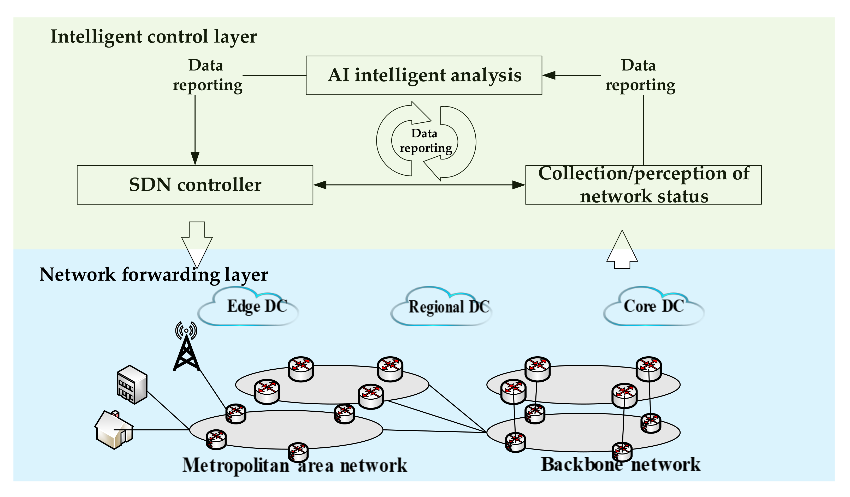
3. Architecture of Intelligent Network Control

By introducing SDN and artificial intelligence technology, the control layer can collect data, analyze the data, generate strategies and issue strategies to form a closed loop of intelligent control. The controller with artificial intelligence function can troubleshoot 90% of network failures and security risks. The architecture of intelligent network control is shown in Figure 1, which mainly includes three parts: the network status collection/perception module, the AI intelligent analysis module and the SDN controller module.

3.1. Collection/Perception of Network Status Module

The collection/perception of the network status module is responsible for collecting network traffic, perceiving network quality and uniformly storing the collected original network data, which can be subscribed by the SDN controller and AI intelligent analysis module. The methods of information collection/perception include: (1) collect link/tunnel traffic information through Telemetry/Snmp/Netconf, (2) collect service flow information through Netflow, (3) collect link/tunnel quality information through TWAMP (Two-Way Active Measurement Protocol).

3.2. AI Intelligent Analysis Module

The AI intelligent analysis module is mainly responsible for obtaining the data processed by the network status collection/perception module, performing intelligent analysis and generating intelligent strategies and issuing SDN controllers for execution. The AI intelligent analysis module has the following capabilities: (1) data adaptation, flexible docking of various data sources; (2) supporting various AI operators such as machine learning, deep learning and reinforcement learning; (3) providing visual AI modeling and pipeline orchestration; (4) the ability to generate intelligent strategies.

3.3. SDN Controller Module

The SDN controller obtains the strategy generated by the AI intelligent analysis module and then calculates the adjustment object and adjustment strategy of the network optimization according to the intelligent network optimization algorithm. The SDN controller sends the calculation result to the network device so as to achieve the purpose of intelligent network control.

4. Research Methods and Solutions

In this paper, we study the traffic optimization case, explore the research method and verify it. It is a challenge to implement the whole network traffic optimization by using SDN controllers based on artificial intelligence. The large-scale adjustment of traffic has a great impact on the network and how to implement it requires research. The problem of entire network traffic optimization is difficult to solve only by traditional methods and traditional routing algorithms. We need to introduce SDN and various AI algorithms represented by machine learning, such as particle swarm optimization, genetic algorithms and simulated annealing algorithms. We designed a network congestion control and prevention algorithm, a resource preemption algorithm and balance of the entire network traffic algorithm based on traditional routing calculation algorithms and AI algorithms. We applied the designed algorithm, artificial intelligence technology and SDN technology to the network to achieve intelligent network control and traffic optimization. The research of this paper is mainly focused on SDN-based network traffic algorithm optimization and experimental verification.

4.1. Object of Flow Optimization

The main objects of traffic optimization are links and tunnels. When the link/tunnel bandwidth utilization exceeds the threshold, the link/tunnel quality drops below the threshold or the tunnel traffic bursts and traffic optimization can be triggered. We can choose the following adjustment objects to adjust:
(1) Link: When there are links congestion in the network, we can optimize the congested links. The optimization methods include (a) increasing the bandwidth of congested links, (b) increasing the transmission links of the congested link, (c) optimizing the tunnel carried by the congested links and changing the transmission paths of the tunnels. We can sort according to the real-time bandwidth of each tunnel carried by the congested link and choose to adjust the top N tunnels for adjustment. In the adjustment process, we must consider the factors such as tunnel priority and tunnel exclusion comprehensively.
(2) Tunnel: When there is tunnel congestion in the network, the adjustment object is the congested tunnel. The optimization methods include (a) increasing the configured tunnel bandwidth and (b) increasing the transmission path of the tunnel, e.g., label switched path (LSP).

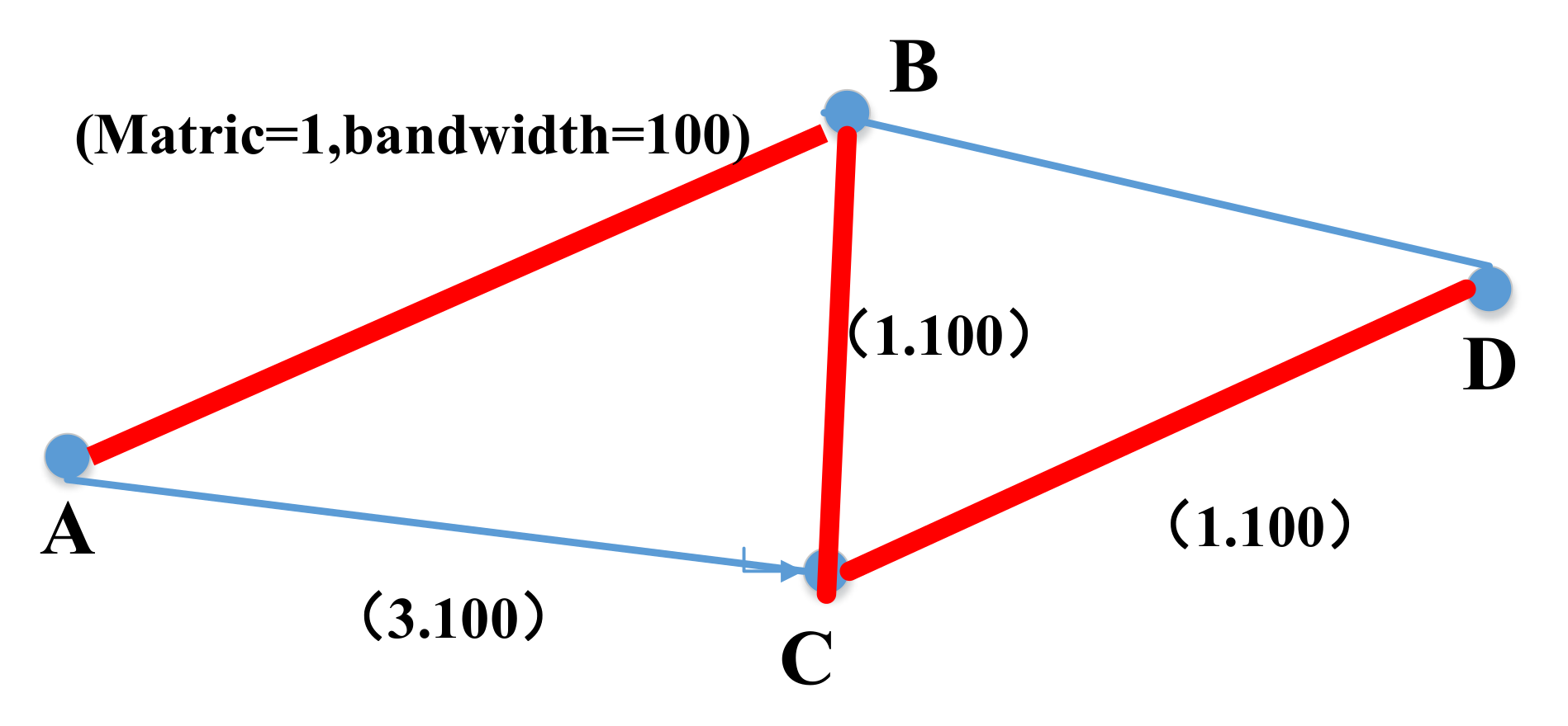
4.2. Routing Calculation Algorithm

4.2.1. GREEDY Algorithm

A greedy algorithm follows the problem-solving heuristic of making the locally optimal choice at each stage [25]. In many problems, a greedy strategy does not usually produce an optimal solution, but nonetheless a greedy heuristic may yield locally optimal solutions that approximate a globally optimal solution in a reasonable amount of time [26].
At present, the greedy algorithm is mainly used for single route calculation. The main calculation strategies include shortest path, minimum delay, maximum bandwidth, load balancing, etc. The typical algorithm of the greedy algorithm is Dijkstra’s algorithm. Dijkstra's algorithm is a path with the smallest weight and the smallest path from a vertex in a topological graph to another vertex, called the shortest path, as shown in the topology in the Figure 2 below.
The attributes on the side represent metric and bandwidth, respectively. Then the calculated optimal path of point A -> D is A -> B -> C -> D, cost = 3.

4.2.2. KSP Algorithm

The k-shortest paths (KSP) algorithm is mainly used to calculate the K optimal path [27]. Its core algorithm is still Dijkstra's algorithm. KSP algorithm realizes K optimal path finding by deleting algorithm. The core of the deletion algorithm is to find the next alternative shortest path by deleting an arc on the shortest path already in the directed graph and looking for an alternative arc. The deletion algorithm is actually implemented by adding additional nodes and corresponding arcs in the directed graph, as shown in the topology in the Figure 3 below.
The attributes on the side represent metric and bandwidth, respectively. Then the calculated two paths when K = 2 at point A -> D is A -> B -> C -> D, cost = 3; A -> C -> D, cost = 4.

4.3. Path Optimization Algorithm

Machine learning is widely used in various application scenarios of network control and optimization, such as network traffic analysis, traffic prediction, abnormal analysis, network simulation and fault diagnosis. Path optimization algorithms mainly include particle swarm algorithms, genetic algorithms, simulated annealing algorithms and other algorithms.

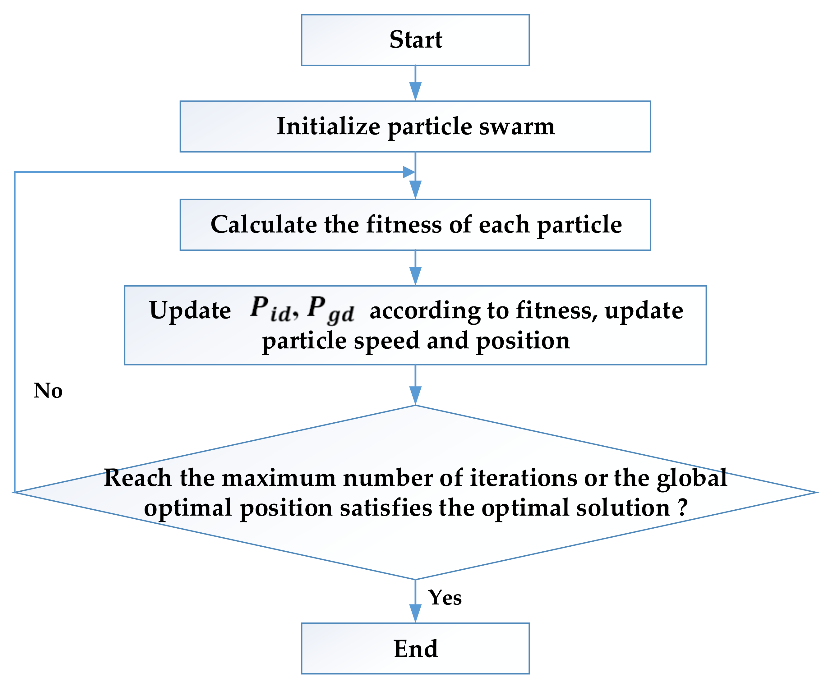
4.3.1. Particle Swarm Optimization

Particle swarm optimization (PSO) was introduced by Kennedy and Eberhart (1995). PSO is a population-based stochastic approach for solving continuous and discrete optimization problems [28].
In particle swarm optimization, particles move in the search space of an optimization problem. The position of a particle represents a candidate solution to the optimization problem at hand [29,30]. Each particle searches for better positions in the search space by changing its velocity according to rules originally inspired by behavioral models of bird flocking. PSO belongs to the class of swarm intelligence techniques that are used to solve optimization problems.
The particles can be dynamically adjusted according to the best historical position of the particles and the best overall historical position. Particles have only two attributes: speed and position. Speed represents the speed of movement, and position represents the direction of movement [31]. The optimal solution searched by each particle is called the individual extremum, and the optimal individual extremum in the particle swarm is regarded as the current global optimal solution. The algorithm continuously iterates, continuously updates the speed and position and finally obtains the optimal solution that satisfies the termination condition [32,33]. The algorithm flow is in Figure 4 as follows:
1. Initialization. We set the maximum number of iterations, the number of independent variables of the objective function, the maximum velocity of the particle and the position information for the entire search space. We initialize the velocity and position randomly on the velocity interval and the search space and set the particle swarm size to M. Each particle randomly initializes a flying speed.
2. Individual extreme value and global optimal solution. Define the fitness function, the individual extreme value is the optimal solution found for each particle, and a global value is found from these optimal solutions, which is called the global optimal solution. The global optimal solution is compared with the historical global optimal solution and updated.
3. Update speed and position formula. The speed and position is computed as follows:
V i d = ω V i d + C 1 r a n d o m 0 , 1 P i d X i d + C 2 r a n d o m 0 , 1 P g d X i d
X i + 1   d = X i d + V i + 1     d      
Among them, ω becomes the inertia factor and its value is non-negative. When it is larger, the global optimization ability is strong, and the local optimization ability is weak. When it is smaller, the global optimization ability is weak, and the local optimization ability is strong. By adjusting the size of ω, the global optimization performance and the local optimization performance can be adjusted. C 1   and   C 2 are called acceleration constants; the former is the individual learning factor of each particle, and the latter is the social learning factor of each particle. A better solution can be obtained when C 1 and   C 2 are constants. We generally takes   C 1   = C 2 0 , 4 , we set C 1   =   C 2   = 2. Random (0,1) represents a random number on the interval [0,1],   P i d represents the d-th dimension of the individual extreme value of the i-th variable, and P g d represents the d-th dimension of the global optimal solution.
4. Termination conditions. (a) Reach the set number of iterations. (b) The difference between the algebras meets the minimum limit.

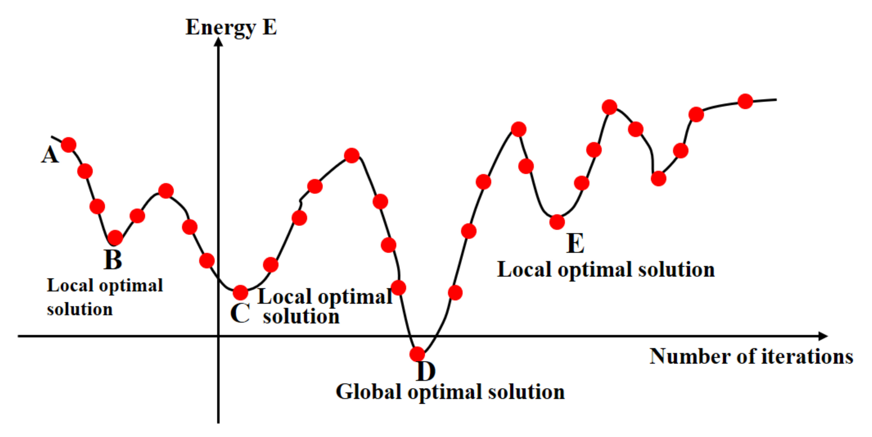
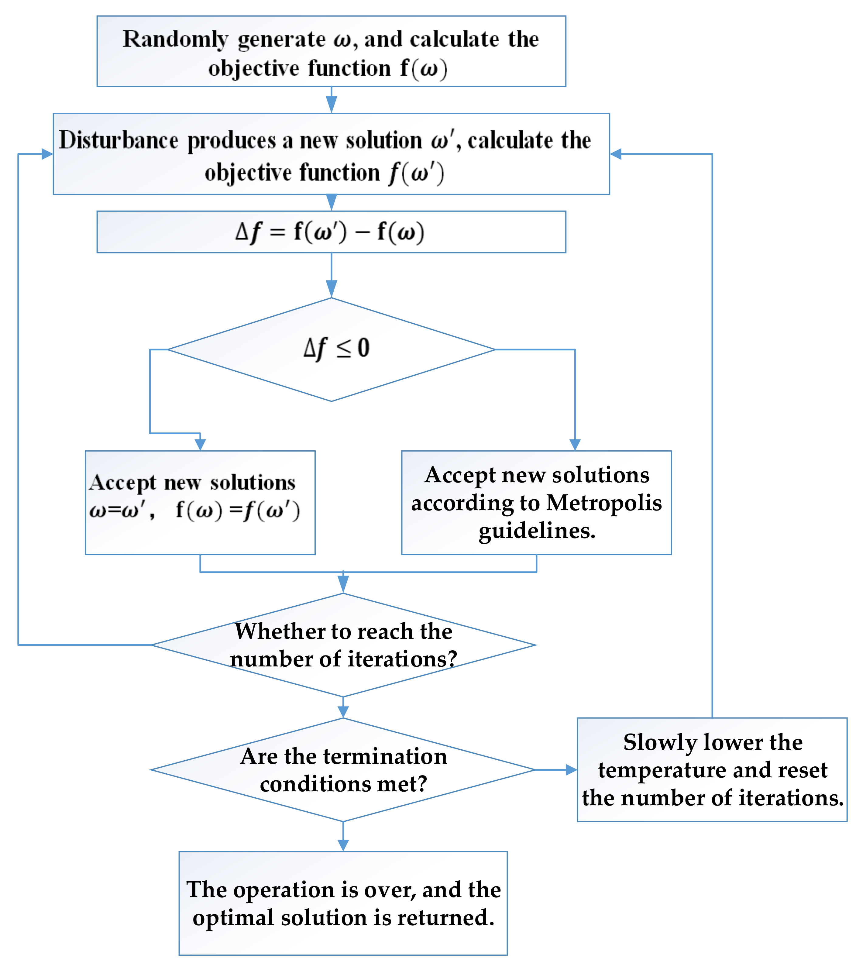
4.3.2. Simulated Annealing

In order to solve the local optimal solution problem, Kirkpatrick et al. proposed the simulated annealing algorithm (SA) in 1983. [34] The simulated annealing algorithm can effectively solve the local optimal solution problem. The simulated annealing algorithm consists of two parts, the metropolis algorithm and the annealing process. The metropolis algorithm is how to make it jump out of the local optimal solution, which is the basis of annealing. Metropolis proposes an importance sampling method, that is, to accept new states with probability instead of using completely certain rules, which is called the Metropolis criterion [35]. This is shown visually in Figure 5 as below:
Assuming that the energy state of the object is at A and iteratively updated to B, B is the local optimal solution. At this time, it is found that when the object is updated to B, the energy of the object is lower than in the A state, which means that it is close to the optimal solution so the state will definitely transfer. After the energy state reaches B, it is found that the energy in the next step has risen. Here, it will jump out of this state with a certain probability. This probability is related to the current state and energy. If it finally jumps out from state B and reaches state C, it will continue to jump out with a certain probability until it reaches state D before it stabilizes [36].
Assuming that the previous state is x(n), the system changes to x(n + 1) according to a certain index. Correspondingly, the energy of the system changes from E(n) to E(n + 1). The acceptance probability P of the system from x(n) to x(n + 1) is defined as (3):
P = 1 ,     E n + 1 < E n e E n + 1 E n T ,     E n + 1 E n  
From the above formula, we can see that if the energy decreases, then this transfer is accepted (P = 1); if the energy increases, it means that the system deviates farther from the global optimal value. At this time, the algorithm will not abandon it immediately, but perform probabilistic operations: first, generate a uniformly distributed random number x in the interval [0,1], if x < P, then this transfer is accepted, otherwise it is rejected and enters the next step. Among them, P is determined by the amount of energy change and T, so the value is dynamic. In the above formula, the adjustable parameter is T. If T is too large, it will anneal too fast, and the iteration will end when the local optimal value is reached. If the value is small, the calculation time will increase. In practical applications, the annealing temperature table is used, and a larger value of T is used in the initial stage of annealing. As the annealing progresses, T is gradually reduced [37]. The specific process is in Figure 6 as follows:
1. The initial temperature T (0) should be selected high enough so that all transition states are accepted.
2. Annealing rate. The simplest way to decline is exponential decline, as shown in Equation (4):
T n + 1 = λ T n ,   n   =   1 , 2 , 3 , 4 ,
where λ is a positive number less than 1 and generally takes a value between 0.8 and 0.99. The convergence speed of exponential decline are relatively slow, and other decline methods are shown in Equations (5) and (6):
T n = T 0 log 1 + t
T n = T 0 1 + t
3. Termination temperature. If there is a new state that can be updated after several iterations or a threshold set by the user is reached, the annealing is complete.

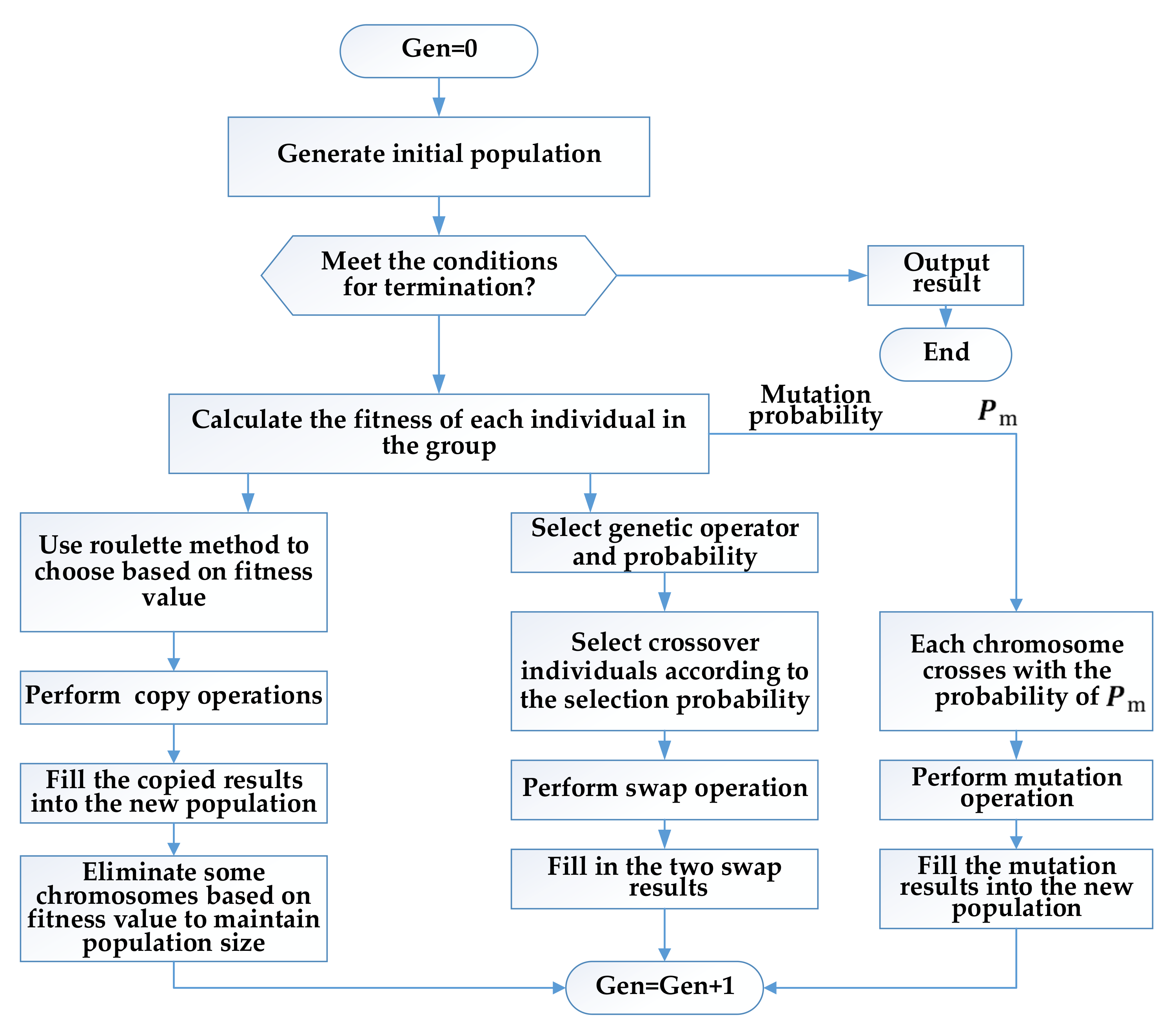
4.3.3. Genetic Algorithm

The Genetic Algorithm (GA) is a heuristic search algorithm that is inspired by Darwin's theory of evolution and draws on the process of biological evolution [38]. Simply put, gene crossover and gene mutation will occur during reproduction; individuals with low fitness will be phased out, and individuals with high fitness will increase their proportion in the population [39]. After N generations of natural selection, the preserved individuals are all highly adaptable, and it is likely to include the individual with the highest adaptability in history [40]. The important concepts of genetic algorithms are given below.
Gene: It is the smallest unit of genetic algorithms. When we write code, it can be a binary bit, such as a real number or a character.
Chromosome: It is the main carrier of genetic material and represents a solution to be solved. A chromosome corresponds to an individual and is composed of multiple genes. It is the basic operating unit of genetic algorithms.
Population: It is composed of a certain number of chromosomes and constitutes the solution space of the problem to be solved, which is the search space of the genetic algorithm.
Fitness: It is a quantitative concept proposed based on the evolutionary principle of "survival of the fittest" in biological evolution theory. It expresses the pros and cons of the solution corresponding to an individual and is often expressed by a fitness function.
Choose: Calculate the fitness value of each individual and use a certain method to select a certain number of good solutions from the previous generation to be inherited by the next generation.
Crossover: Partial genes of two chromosomes are exchanged to produce a new generation of individuals. This process embodies the idea of information crossover and is the most important genetic operation in genetic algorithms.
Mutation: Change the gene value in an individual according to the size of the mutation factor to produce a new generation of individuals.
The algorithm flow of genetic algorithms is in Figure 7, as follows:
1. Randomly generate a population as the first generation solution of the problem.
2. Find a suitable coding scheme to code individuals in the population; one can choose common coding schemes such as floating-point number coding or binary coding.
3. Take the function value of the multimodal function as the fitness of the individual and calculate the fitness of each individual in the population. We choose a function which is expressed as the following:
F = i = 1 N F i c i k N
where N is the number of used operation rooms (OR) in the solution, F i   is the sum of all the surgeries to be perform in bin i , c i   is the capacity of the i-th-OR and k is a constant (k > 1).
4. According to the level of fitness, choose the two parents to participate in the reproduction. The principle of selection is that the higher the fitness, the more likely it is to be selected.
5. Perform genetic operations on the selected two parents; that is, copy the genes of the two parents and use crossover, mutation and other operators to produce offspring.
6. According to certain criteria, judge whether to continue to execute the algorithm or to find the individual with the highest fitness among all offspring to return as the solution and end the program. The theoretical optimum determines which would be the minimal quantity of ORs needed to schedule a set of activities. This value is expressed by (8):
x t , i = 1 + x t c i ,   i + 1             if   t = 0 0                                           if   t 0
where
t is the summation of the duration of all activities to schedule;
i is a control parameter, and c i   is the capacity.

4.4. Network Congestion Control and Prevention Algorithm

When we optimize the network traffic, we must consider the minimum number of services adjustments in the network, the balance of link bandwidth utilization and the balance between services adjustments and link bandwidth utilization.
Traffic optimization is performed on the actual traffic in the current time period, with the purpose of reducing the bandwidth utilization of congested links. We use the congested link as the exclusion node constraint and calculate the relatively short path based on the Dijkstra’s algorithm to bypass the congested path and at the same time use the genetic algorithm to optimize. The specific process is as follows:
(a) According to the congestion threshold, we look for congested links and adjustable services on congested links.
(b) For congested services, we take the initial congested link as a best-effort exclusion node and calculate N adjustable paths based on the Dijkstra's algorithm.
(c) We perform several random combinations on the calculated path and ensure that the planning bandwidth does not exceed the limit and then use it as the initial population of the genetic algorithm. Then, the genetic iteration is according to the following three conditions:
  • The number of service adjustments is the least. The genetic algorithm population always chooses the standard solution that has less disturbance with the offspring's inheritance and cross mutation. After several iterations, we chose the solution with the least disturbance to return and deploy.
  • The link utilization rate is the most balanced after adjustment. The genetic algorithm population always chooses a solution with lower link utilization rate for offspring genetic and cross mutation. After several iterations, choose the solution with the lower maximum utilization rate to return and deploy.
  • After adjustment, the link utilization is the most balanced, and the number of adjusted services is the least. The genetic algorithm population always selects the solution with the smallest maximum utilization and less disturbance for offspring inheritance and cross mutation. Then, the solution with the smaller maximum utilization and smaller disturbance is selected as the return deployment plan.

4.5. Resource Preemption Algorithm

In the process of opening new tunnel services or optimizing tunnels, service deployment problems may arise. When we open new tunnel services and calculate service requests in the existing network, the path calculation will fail due to insufficient remaining bandwidth of the network. When we are optimizing congested services, the link will still be congested after optimization; that is, the effect of optimization is not obvious. In view of these two common situations, we designed an algorithm for resource preemption based on request priority. This algorithm allows high-priority requests to preempt the path of low-priority requests and tries to meet the deployment of high-priority requests. The algorithm steps are as follows:
(a) According to the priority threshold, we filter the high-priority requests that need to be preempted and sort these high-priority requests one by one from high to low.
(b) For a single high-priority request, we find a set of links with insufficient bandwidth or congestion in its path and establish a mapping relationship between the links in the set and the low-priority requests involved.
(c) According to the preemption requirements, we divide the following three situations to preempt:
  • The number of disturbed services is the least during preemption. We select the low-priority request to be dismantled, optimize it with a heuristic algorithm and set the minimum number of dismantlement request services as the optimization goal. We iterate the algorithm until the algorithm converges and finally return the collection of low priority requests to be dismantled.
  • Preempt low-priority services. We select the low-priority requests to be removed, optimize them with heuristic algorithms and set the minimum sum of low-priority requests to be removed as the optimization goal. We iterate the algorithm until the algorithm converges and finally return the collection of low priority requests for removal.
  • The balance between the number of preempted services and the priority of preempted services. We select the low-priority request to be removed, optimize it with a heuristic algorithm and assign different weight coefficients to the number and priority of the removed service. Then, we take the smallest sum as the optimization goal. We iterate the algorithm until the algorithm converges and finally return the collection of low priority requests to be removed.

4.6. Balance of the Entire Network Traffic Algorithm

When the deployment of services in the network is inappropriate, it will result in a large bandwidth occupation, a large product of bandwidth and delay or a large product of bandwidth and cost. In response to these problems, we have designed an algorithm that can optimize the bandwidth usage of the entire network, the bandwidth and delay of the entire network and the bandwidth and cost of the entire network. When all requests are successfully deployed in the current network, we use this algorithm to optimize the network to achieve reducing the bandwidth occupancy value, reducing the sum of the bandwidth and the delay product, and improving the network performance. The performance of the optimized network will be improved compared with that before optimization. The algorithm combines the characteristics of the greedy algorithm and heuristic algorithm. The steps are as follows:
(a) Find and filter the services that can be adjusted. For the services that have been deployed in the current network, we filter the services that can be adjusted according to the priority threshold except for services that require path protection and cannot be adjusted, and then follow the priority and the bandwidth size to sort the services.
(b) According to the goal of network optimization, we divide the following three situations to optimize the algorithm.
  • Occupies the smallest bandwidth. We adopt the open corporate strategy and program framework (Open-CSPF) in the calculation of the service path, set the weight reader as the hop reader, and the path calculation for each service is carried out according to the principle of the smallest hop. We perform path calculations for the services in step (a) one by one and deploy them into the network to obtain a better solution. On the basis of this solution, we introduce a heuristic algorithm, multiply the bandwidth of the network by the number of hops and sum them. The sum is used to measure the performance of the solution. We look for a better solution until the algorithm converges and return to the final solution.
  • Minimal cost: We adopt the Open-CSPF in the calculation of the service path, set the weight reader as the cost reader, and the path calculation for each service is performed according to the principle of minimum cost. We calculate the paths of the services in step (a) one by one and deploy them into the network to obtain a better solution. On the basis of this solution, we introduce a heuristic algorithm to multiply the network bandwidth by the cost and sum it up; the sum is used to measure the performance of the solution. We look for a better solution until the algorithm converges and return the final solution.
  • Minimal delay: We adopt the Open-CSPF in the calculation of the services path, set the weight reader as the delay reader, and the path calculation for each service is performed according to the principle of minimum delay. We calculate the paths of the services in step (a) one by one and deploy them into the network to obtain a better solution. On the basis of this solution, we introduce a heuristic algorithm to multiply the network bandwidth by the delay and sum; the sum is used to measure the performance of the solution. We look for a better solution until the algorithm converges and return to the final solution.
In order to optimize the bandwidth load balance of the entire network in the offline state, we adopt the greedy algorithm and genetic algorithm. The process is as follows:
(a) Keep the request and path information before we optimize and store it in the initial fill.
(b) Select the requests to be optimized and then sort the requests to be optimized according to the priority and bandwidth value to ensure that the services paths with high priority and large bandwidth are calculated first.
(c) Based on the single-path BwLB algorithm, we pre-allocate an optional path for each request and use it as the initial population of the genetic algorithm.
(d) We adopt genetic algorithms to perform crossover, mutation and selection operations on the initial population, continuously generate new chromosomes and keep better chromosomes to continue crossover and mutation. We continue to iterate until the end of the algorithm and select the best chromosome from the final population as a feasible solution for the batch path.
(e) If the bandwidth utilization of the optimal chromosome is not better than the result before optimization, the return path optimization fails. If it is better than the result before optimization, the optimization success is returned.

5. Experimental Validation

5.1. Traffic Optimization Case Analysis

We give the network topology as shown in Figure 8:
The information of the initial network is as shown in Table 1:
Attributes of service request are as shown in Table 2:
Based on the above information, we give three optimization scenarios: (a) maximum utilization of network resources, (b) congestion control and prevention, (c) resource load sharing.

5.1.1. Maximum Utilization of Network Resources

The status of service deployment before service optimization is shown in Table 3 below.
The features of service deployment before service optimization are as follows: (a) the utilization rate of Link A -> C is 60%, (b) the utilization rate of links A -> B and B -> C are all zero, (c) the link load is unbalanced.
We use algorithms that maximize the utilization of network resources for network optimization. The optimized service deployment status is shown in Table 4 below.
The features of service deployment after services optimization are as follows: (a) the bandwidth utilization rate of link A -> C is the largest, which is 33.3%; (b) the utilization rate of link A -> B and B -> C is 26.7%; (c) the link load is balanced.

5.1.2. Congestion Control and Prevention

We assume the following network conditions: (a) services have been deployed in the network; (b) the corresponding services attributes and deployment methods are shown in Figure 8 and Table 4, respectively; (c) at this time, there is a new service 4 request that needs to be deployed into the network: the size is 120 M, the starting point is S1, and the end point is E1.
The network status now is as follows: (a) whether the service 4 passes through path 1 or path 2, it will cause link congestion; (b) the transmission path of one or several of the first three services needs to be adjusted; (c) ensure that service 4 can be successfully deployed into the network; (d) make the entire network in a balanced state.
We use congestion control and prevention algorithms for optimization. The results of path optimization are shown in Table 5 below:
The comparison of the path optimization from Table 4 to Table 5 is as follows: (a) the transmission path of service 2 and 3 has changed; (b) the deployment of service 4 is guaranteed; (c) the bandwidth utilization of each link is 60%, 60% and 80%, which is the best balance that the network can achieve.

5.1.3. Resource Load Sharing

We assume the following network conditions: (a) three services have been deployed in the network; (b) the corresponding service attributes and deployment methods are shown in Figure 8 and Table 4, respectively; (c) there is a new service 4 request that needs to be deployed into the network. The bandwidth of this service is 150 M, the starting point is S1, and the end point is E1.
We can find the following situations in the existing network status: (a) service 4 cannot be successfully deployed even if the above-mentioned "congestion control and prevention" technology is used; (b) we can consider the manner of resource load sharing and use the remaining fragmented resources to carry more services; that is, service 4 will be split and transmitted.
We use resource load sharing algorithms for optimization. The results of path optimization are shown in Table 6 below:
The network status after path optimization is as follows: (a) service 4 is split into service 5 and service 6 for transmission; (b) the bandwidth of service 5 and service 6 are 80 M and 70 M, respectively; (c) the bandwidth utilization of each link of the network is the same.

5.2. Traffic Optimization Verification

We use a mesh topology network of 500 nodes to verify the capabilities of the algorithm. We first randomly generate points A and Z and establish 1000 test tunnels between points A and Z. The optimization strategies adopt global load balancing strategies, load balancing and disturbance control strategies. The test server is configured as WIN7 CPU8, 6G Memory; the strategies’ convergence speed is seconds.
We conducted ten sets of tests, each of which randomly generated 1000 tunnels. We set the link utilization threshold to be 50%. The adjustment strategies adopted load balancing. The goal of algorithm optimization was to try to reduce the maximum link utilization. From the Table 7 below, we can see that the link utilization rate can finally be reduced below the target threshold, but the number of adjusted services and the disturbance rate is large. We still reused the ten sets of requests, set the utilization threshold to 50% and changed the adjustment strategies to load balancing and disturbance control. The algorithm optimization goal is to control disturbances and reduce the maximum utilization as much as possible. As shown in Table 8 below, it can be seen that the utilization rate can be reduced, and the disturbance becomes relatively small; the final utilization rate is a little higher than that shown in Table 7.

6. Conclusions

In this paper, we designed a network control mechanism for network intelligent control and solutions for traffic optimization based on SDN and artificial intelligence. We propose an intelligent network control architecture based on SDN and artificial intelligence. Additionally, this paper also analyzes the objectives of traffic optimization as well as routing calculation algorithms and routing optimization algorithms. In addition, we also put forward three optimization algorithms for the operator’s network. Finally, we conduct experiments to verify the effectiveness of the control mechanism and algorithms. The experimental results show that the use of SDN and artificial intelligence in operator networks can realize network intelligent control and traffic optimization more intelligently.
In this paper, the system is only evaluated on synthetic data so it is difficult to know whether it would perform well in an actual situation. Hence, in future we will try to apply network intelligent control and traffic optimization based on SDN and artificial intelligence solutions to operators' actual networks in order to solve real data problems in future work; at the same time, more network intelligent control application scenarios will be studied.
By introducing artificial intelligence technology into the operators’ network, the SDN controller can provide a more flexible, accurate and dynamic traffic scheduling method. Based on different traffic characteristics, it can dynamically schedule different flows to different paths, which significantly improves the use of network resources, effectively reducing the load of network equipment and enhancing network scalability and flexibility. In all, since optimization for this type of autonomous control will no doubt be more common in the future, the proposed method provides an effective solution for solving the network traffic optimization problem of operators.

Author Contributions

Conceptualization, A.G., C.Y.; methodology and validation, A.G.; discussion and final editing, A.G.; writing—review and editing, A.G., C.Y. All authors have read and agreed to the published version of the manuscript.

Funding

This research received no external funding

Data Availability Statement

All data included in this study are available upon request by contact with the corresponding author.

Conflicts of Interest

The authors declare no conflict of interest.

References

  1. Valadarsky, A.; Schapira, M.; Shahaf, D.; Tamar, A. Learning to Route. In Proceedings of the 16th ACM Workshop on Hot Topics in Networks (HotNets-XVI), Palo Alto, CA, USA, 30 November–1 December 2017; ACM: New York, NY, USA, 2017; pp. 185–191. [Google Scholar]
  2. Bai, H. A Survey on Artificial Intelligence for Network Routing Problems; University of New Mexico: Albuquerque, NM, USA, 2007. [Google Scholar]
  3. Fortz, B.; Rexford, J.; Thorup, M. Traffic engineering with traditional IP routing protocols. Comm. Mag. 2002, 40, 118–124. [Google Scholar] [CrossRef] [Green Version]
  4. Kandula, S.; Katabi, D.; Davie, B.; Charny, A. Walking the tightrope. ACM SIGCOMM Comput. Commun. Rev. 2005, 35, 253–264. [Google Scholar] [CrossRef]
  5. Kumar, P.; Yuan, Y.; Yu, C.; Foster, N.; Kleinberg, R.D.; Soulé, R. Kulfi: Robust Traffic Engineering Using Semi-Oblivious Routing. Available online: https://arxiv.org/pdf/1603.01203.pdf (accessed on 3 March 2016).
  6. Yousaf, F.Z.; Bredel, M.; Schaller, S.; Schneider, F. NFV and SDN—Key technology enablers for 5G networks. IEEE J. Sel. Areas Commun. 2017, 35, 2468–2478. [Google Scholar] [CrossRef] [Green Version]
  7. Wang, S.Y. Comparison of SDN OpenFlow network simulator and emulators: EstiNet vs. Mininet. In Proceedings of the IEEE Symposium on Computers and Communications, Funchal, Portugal, 23–26 June 2014; pp. 1–6. [Google Scholar]
  8. Mostafaei, H.; Lospoto, G.; di Lallo, R.; Rimondini, M.; di Battista, G. A framework for multi-provider virtual private networks in software-defined federated networks. Int. J. Netw. Manag. 2020, 30, e2116. [Google Scholar] [CrossRef]
  9. Gouveia, R.; Aparício, J.; Soares, J.; Parreira, B.; Sargento, S.; Carapinha, J. SDN framework for connectivity services. In Proceedings of the IEEE International Conference on Communications, Sydney, Australia, 10–14 June 2014; pp. 3058–3063. [Google Scholar]
  10. Benzekki, K.; El Fergougui, A.; Elbelrhiti Elalaoui, A. Software-defined networking (SDN): A survey. Secur. Commun. Netw. 2016, 9, 5803–5833. [Google Scholar] [CrossRef]
  11. Khan, S.; Gani, A.; Wahab, A.W.A.; Guizani, M.; Khan, M.K. Topology discovery in software defined networks: Threats, taxonomy, and state-of-the-art. IEEE Commun. Surv. Tutor. 2017, 19, 303–324. [Google Scholar] [CrossRef]
  12. SDN White Paper. Available online: https://www.opennetworking.org/download-after/sdn-transport-api-interoperability-demonstration-executive-overview-technical-white-paper-download/ (accessed on 28 November 2019).
  13. Open Networking Foundation (ONF). Available online: https://www.opennetworking.org/ (accessed on 28 November 2019).
  14. Feamster, N.; Rexford, J.; Zegura, E. The road to SDN. ACM SIGCOMM Comput. Commun. Rev. 2014, 44, 87–98. [Google Scholar] [CrossRef]
  15. Oloduowo, A.; Babalola, A.H.; Daniel, A.K. Solving Network Routing Problem Using Artificial Intelligent Techniques. Br. J. Math. Comput. Sci. 2016, 17, 1–9. [Google Scholar] [CrossRef]
  16. Fadlullah, Z.M.; Tang, F.; Mao, B.; Kato, N.; Akashi, O.; Inoue, T.; Mizutani, K. State-of-the-art deep learning: Evolving machine intelligence toward tomorrow’s intelligent network traffic control systems. IEEE Commun. Surv. Tutor. 2017, 19, 2432–2455. [Google Scholar] [CrossRef]
  17. Qadir, J. Artificial intelligence based cognitive routing for cognitive radio networks. Artif. Intell. Rev. 2016, 45, 25–96. [Google Scholar] [CrossRef] [Green Version]
  18. Wu, Y.-J.; Hwang, P.-C.; Hwang, W.-S.; Cheng, M.-H. Artificial Intelligence Enabled Routing in Software Defined Networking. Appl. Sci. 2020, 10, 6564. [Google Scholar] [CrossRef]
  19. Mata, J.; de Miguel, I.; Durán, R.J.; Merayo, N.; Singh, S.K.; Jukan, A.; Chamania, M. Artificial intelligence (AI) methods in optical networks: A comprehensive survey. Opt. Switch. Netw. 2018, 28, 43–57. [Google Scholar] [CrossRef]
  20. Mao, B.; Fadlullah, Z.M.; Tang, F.; Kato, N.; Akashi, O.; Inoue, T.; Mizutani, K. Routing or computing? The paradigm shifts towards intelligent computer network packet transmission based on deep learning. IEEE Trans. Comput. 2017, 66, 1946–1960. [Google Scholar] [CrossRef]
  21. Al-Fares, M.; Radhakrishnan, S.; Raghavan, B.; Huang, N.; Vahdat, A. Hedera: Dynamic Flow Scheduling for Data Center Networks. In Proceedings of the 7th USENIX Conference on Networked Systems Design and Implementation, San Jose, CA, USA, 28–30 April 2010. [Google Scholar]
  22. Barbancho, J.; León, C.; Molina, F.J.; Barbancho, A. Using artificial intelligence in routing schemes for wireless networks. Comput. Commun. 2007, 30, 2802–2811. [Google Scholar] [CrossRef]
  23. Panno, D.; Riolo, S. An enhanced joint scheduling scheme for GBR and non-GBR services in 5G RAN. Wirel. Netw. 2020, 26, 3033–3052. [Google Scholar] [CrossRef]
  24. Ye, Y.; Fang, H.; Nie, D. Optimization and application of 5G bearer network backhaul bandwidth estimation model. Telecommun. Sci. 2020, 36, 138–143. [Google Scholar]
  25. Black, P.E. Dictionary of Algorithms and Data Structures; U.S. National Institute of Standards and Technology (NIST): Gaithersburg, MD, USA, 2012. [Google Scholar]
  26. Bang-Jensen, J.; Gutin, G.; Yeo, A. When the greedy algorithm fails. Discret. Optim. 2004, 1, 121–127. [Google Scholar] [CrossRef] [Green Version]
  27. Yen, J.Y. An algorithm for finding shortest routes from all source nodes to a given destination in general networks. Q. Appl. Math. 1970, 27, 526–530. [Google Scholar] [CrossRef] [Green Version]
  28. Zungeru, A.M.; Ang, L.; Seng, K.P. Classical and swarm intelligence based routing protocols for wireless sensor networks: A survey and comparison. J. Netw. Comput. Appl. 2012, 35, 1508–1536. [Google Scholar] [CrossRef]
  29. Willmott, S.; Faltings, B.; Frei, C.; Calisti, M. Organization and Coordination for On-Line Routing in Communications Networks. In Software Agents for Future Communication Systems; Hayzelden, A.L.G., Bigham, J., Eds.; Springer: Berlin/Heidelberg, Germany, 1999. [Google Scholar]
  30. Dorigo, M. Particle swarm optimization. Scholarpedia 2008, 3, 1486. [Google Scholar] [CrossRef]
  31. Clerc, M. Particle Swarm Optimization; ISTE: London, UK, 2006. [Google Scholar]
  32. Clerc, M.; Kennedy, J. The particle swarm-explosion, stability and convergence in a multidimensional complex space. IEEE Trans. Evol. Comput. 2002, 6, 58–73. [Google Scholar] [CrossRef] [Green Version]
  33. Engelbrecht, A.P. Fundamentals of Computational Swarm Intelligence; John Wiley & Sons: Chichester, UK, 2005. [Google Scholar]
  34. Henderson, D.; Jacobson, S.H.; Johnson, A.W. The Theory and Practice of Simulated Annealing. In Handbook of Metaheuristics; International Series in Operations Research & Management, Science; Glover, F., Kochenberger, G.A., Eds.; Springer: Boston, MA, USA, 2003; Volume 57. [Google Scholar]
  35. Laarhoven, P.; Aarts, E. Simulated Annealing: Theory and Applications; Springer: Dordrecht, The Netherlands, 1987. [Google Scholar]
  36. Ledesma, S.; Ruiz, J.; Garcia, G. Simulated Annealing Evolution, Simulated Annealing—Advances, Applications and Hybridizations, Marcos de Sales Guerra Tsuzuki; IntechOpen: London, UK, 2012; Available online: https://www.intechopen.com/books/simulated-annealing-advances-applications-and-hybridizations/simulated-annealing-evolution (accessed on 29 August 2012).
  37. Askarzadeh, A.; Coelho, L.d.S.; Klein, C.E.; Mariani, V.C. A population-based simulated annealing algorithm for global optimization. In Proceedings of the 2016 IEEE International Conference on Systems, Man, and Cybernetics (SMC), Budapest, Hungary, 9–12 October 2016; pp. 4626–4633. [Google Scholar]
  38. Jennings, P.C.; Lysgaard, S.; Hummelshøj, J.S.; Vegge, T.; Bligaard, T. Genetic algorithms for computational materials discovery accelerated by machine learning. Npj Comput. Mater. 2019, 5, 46. [Google Scholar] [CrossRef]
  39. Katoch, S.; Chauhan, S.S.; Kumar, V. A review on genetic algorithm: Past, present, and future. Multimedia Tools Appl. 2021, 80, 8091–8126. [Google Scholar] [CrossRef] [PubMed]
  40. Ohn, H. Holland: Genetic algorithms. Scholarpedia 2012, 7, 1482. [Google Scholar]
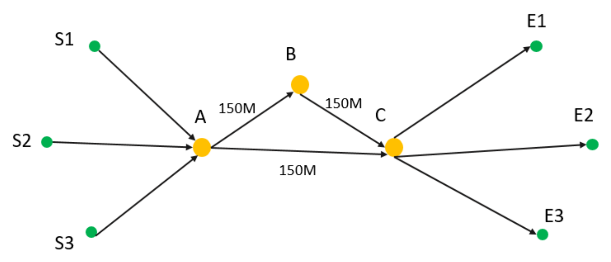
Figure 1. Architecture of intelligent network control.
Electronics 10 00700 g001
Figure 2. Dijkstra’s algorithm diagram.
Electronics 10 00700 g002
Figure 3. KSP algorithm diagram.
Electronics 10 00700 g003
Figure 4. Particle swarm algorithm process.
Electronics 10 00700 g004
Figure 5. Schematic diagram of the annealing algorithm.
Electronics 10 00700 g005
Figure 6. Process of simulated annealing.
Electronics 10 00700 g006
Figure 7. Algorithm flow of genetic algorithms.
Electronics 10 00700 g007
Figure 8. Network topology.
Electronics 10 00700 g008
Table 1. Initial information of network.
Path 1S1 -> A -> B -> C -> E1
Path 2S1 -> A -> C -> E1
Path 3S2 -> A -> B -> C -> E2
Path 4S2 -> A -> C -> E2
Path 5S3 -> A -> B -> C -> E3
Path 6S3 -> A -> C -> E3
Table 2. Attributes of service request.
ServiceStart PointEnd PointSize
Service 1S1E140 M
Service 2S2E230 M
Service 3S3E320 M
Table 3. Status of service deployment before optimization.
Scheme Path 1Path 2Path 3Path 4Path 5Path 6Maximum Link
Utilization
Service 1 60%
Service 2
Service 3
Table 4. Status of service deployment after optimization.
ServicePath 1Path 2Path 3Path 4Path 5Path 6Maximum Link
Utilization
Service 1 33.3%
Service 2
Service 3
Table 5. Service status after path optimization.
ServicePath 1Path 2Path 3Path 4Path 5Path 6Maximum Link
Utilization
Service 1 80%
Service 2
Service 3
Service 4
Table 6. Service status after path optimization.
ServicePath 1Path 2Path 3Path 4Path 5Path 6Maximum Link
Utilization
Service 1 80%
Service 2
Service 3
Service 5
Service 6
Table 7. Verification of traffic optimization based on load balancing strategies.
Testing ScenariosCongestion ThresholdOriginal Highest Link UtilizationNumber of Congested LinksNumber of Congested ServicesConvergence Time
(Less Than)
Disturbance is Not Considered: Reduce Link Utilization,
Regardless of the Number of Services
Maximum Link
Utilization
after
Optimization
Number of Adjusted
Services
Number of Adjusted LinksRemaining Congested LinksNumber of Remaining Congested Services
case 150%56.32%643110 s41.11%374908800
case 255%77.66%1463410 s53.59%59212,05500
case 350%72.49%1454710 s42.92%44412,65800
case 450%78.65%1355510 s44.91%46312,64000
case 550%75.63%1466710 s48.14%50412,85900
case 650%77.43%1358610 s44.39%46212,61900
case 750%62.41%934210 s42.57%340947100
case 850%76.18%1654110 s44.76%42112,04300
case 950%91.76%1047210 s49.61%44011,80900
case 1050%72.66%1860610 s45.14%48412,42100
Table 8. Verification of traffic optimization based on load balancing and disturbance control strategies.
Testing
Scenarios
Congestion ThresholdOriginal Highest Link UtilizationNumber of Congested LinksNumber of Congested ServicesConvergence Time
(Less Than)
Consider Disturbance: Reduce Link Utilization and Fewer Service Adjustments
Maximum Link
Utilization
after
Optimization
Number of Adjusted
Services
Number of Adjusted LinksRemaining Congested LinksNumber of Remaining Congested Services
case 150%56.32%643110 s44.70%123359400
case 255%77.66%1463410 s52.07%245493200
case 350%72.49%1454710 s46.09%219580400
case 450%78.65%1355510 s47.92%187510900
case 550%75.63%1466710 s49.30%273624100
case 650%77.43%1358610 s45.43%231593100
case 750%62.41%934210 s44.41%110308000
case 850%76.18%1654110 s45.80%227600200
case 955%91.76%1047210 s55.00%187501300
case 1050%72.66%1860610 s48.42%214584900
Publisher’s Note: MDPI stays neutral with regard to jurisdictional claims in published maps and institutional affiliations.

