
A Hybrid Supervised Machine Learning Classifier System for Breast Cancer Prognosis Using Feature Selection and Data Imbalance Handling Approaches


 ,
,  ,
,  , ,
, ,  and
and
Abstract
1. Introduction
2. Materials and Methods
2.1. Dataset and Tools
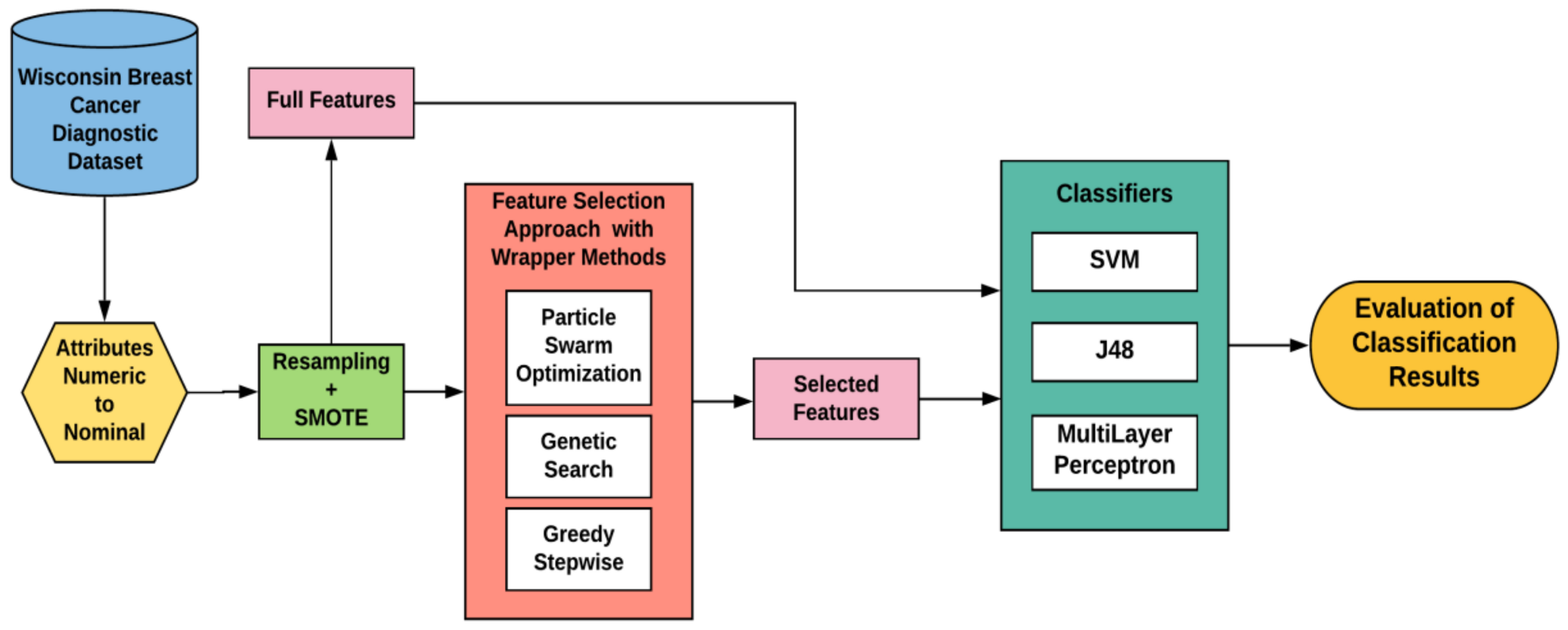
2.2. Methodology for the Proposed System
2.2.1. Data Pre-Processing
2.2.2. Data Imbalance Handling
2.2.3. Feature Selection Algorithms
Particle Swarm Optimization
Genetic Search
Greedy Stepwise
2.2.4. Machine Learning Classifiers
Support Vector Machine
J48
Multilayer Perceptron
2.2.5. Performance Evaluation Metrics
Classification Accuracy
Sensitivity
Specificity
Matthew’s Correlation Coefficient
Kappa Statistics
- P0: Probability of agreement.
- Pe: Probability of random agreement
3. Results
4. Discussion
5. Conclusions
Author Contributions
Funding
Conflicts of Interest
References
- Wu, J.; Mamidi, T.K.K.; Zhang, L.; Hicks, C. Unraveling the Genomic-Epigenomic Interaction Landscape in Triple Negative and Non-Triple Negative Breast Cancer. Cancers 2020, 12, 1559. [Google Scholar] [CrossRef] [PubMed]
- Siegel, R.L.; Miller, K.D.; Jemal, A. Cancer statistics, 2019. CA. Cancer J. Clin. 2019, 69, 7–34. [Google Scholar] [CrossRef] [PubMed]
- Gupta, G.; Dang, R.; Gupta, S. Clinical presentations of carcinoma breast in rural population of North India: A prospective observational study. Int. Surg. J. 2019, 6, 1622–1635. [Google Scholar] [CrossRef]
- Kalarivayil, R.; Desai, P.N. Emerging technologies and innovation policies in India: How disparities in cancer research might be furthering health inequities? J. Asian Public Policy 2020, 13, 192–207. [Google Scholar] [CrossRef]
- Raina, V.; Deo, S.; Shukla, N.; Mohanti, B.; Gogia, A. Triple-negative breast cancer: An institutional analysis. Indian J. Cancer 2014, 51, 163–178. [Google Scholar] [CrossRef]
- Roy, S.; Kumar, R.; Mittal, V.; Gupta, D. Classification models for Invasive Ductal Carcinoma Progression, based on gene expression data-trained supervised machine learning. Sci. Rep. 2020, 10, 4113–4126. [Google Scholar] [CrossRef]
- Saba, T. Recent advancement in cancer detection using machine learning: Systematic survey of decades, comparisons and challenges. J. Infect. Public Health 2020, 13, 1274–1289. [Google Scholar] [CrossRef] [PubMed]
- Chakravarthy, S.R.S.; Rajaguru, H. Detection and classification of microcalcification from digital mammograms with firefly algorithm, extreme learning machine and non-linear regression models: A comparison. Int. J. Imaging Syst. Technol. 2020, 30, 126–146. [Google Scholar] [CrossRef]
- Eedi, H.; Kolla, M. Machine Learning aproaches for healthcare data analysis. J. Crit. Rev. 2020, 7, 312–326. [Google Scholar] [CrossRef]
- Saoud, H.; Ghadi, A.; Ghailani, M.; Boudhir, A.A. Application of data mining classification algorithms for breast cancer diagnosis. ACM Int. Conf. Proc. Ser. 2018, 20, 34–46. [Google Scholar] [CrossRef]
- Saoud, H.; Ghadi, A.; Ghailani, M. Proposed approach for breast cancer diagnosis using machine learning. ACM Int. Conf. Proc. Ser. 2019, 21, 1–5. [Google Scholar] [CrossRef]
- Domingo, M.J.; Gerardo, B.D.; Medina, R.P. Fuzzy decision tree for breast cancer prediction. ACM Int. Conf. Proc. Ser. 2019, 12, 316–328. [Google Scholar] [CrossRef]
- Sahu, B.; Panigrahi, A. Efficient Role of Machine Learning Classifiers in the Prediction and Detection of Breast Cancer. SSRN Electron. J. 2020, 10, 1–9. [Google Scholar] [CrossRef]
- Al-Shargabi, B.; Al-Shami, F. An experimental study for breast cancer prediction algorithms. ACM Int. Conf. Proc. Ser. 2019, 21, 3–8. [Google Scholar] [CrossRef]
- Zhang, J.; Chen, L.; Abid, F. Prediction of Breast Cancer from Imbalance Respect Using Cluster-Based Undersampling Method. J. Healthc. Eng. 2019, 2019. [Google Scholar] [CrossRef]
- Prabadevi, B.; Deepa, K.L.B.N.; Vinod, V. Analysis of Machine Learning Algorithms on Cancer Dataset. In Proceedings of the 2020 International Conference on Emerging Trends in Information Technology and Engineering (ic-ETITE), Vellore, India, 24–25 February 2020; pp. 1–10. [Google Scholar] [CrossRef]
- Fotouhi, S.; Asadi, S.; Kattan, M.W. A comprehensive data level analysis for cancer diagnosis on imbalanced data. J. Biomed. Inform. 2019, 90, 103089. [Google Scholar] [CrossRef] [PubMed]
- Haq, A.U.; Li, J.P.; Memon, M.H.; Nazir, S.; Sun, R.; Garciá-Magarinõ, I. A hybrid intelligent system framework for the prediction of heart disease using machine learning algorithms. Mob. Inf. Syst. 2018, 2018. [Google Scholar] [CrossRef]
- Farid, A.A.; Selim, G.I.; Khater, H.A. A Composite Hybrid Feature Selection Learning-Based Optimization of Genetic Algorithm for Breast Cancer Detection. Preprints 2020, 25, 1–21. [Google Scholar] [CrossRef]
- Sahu, B.; Panigrahi, A.; Mohanty, S.; Sobhan, S. A hybrid Cancer Classification Based on SVM Optimized by PSO and Reverse Firefly Algorithm. Int. J. Control Autom. 2020, 13, 506–517. [Google Scholar]
- Sahu, B.; Mohanty, S.N.; Rout, S.K. EAI Endorsed Transactions on Scalable Information System s A H ybrid Approach for Breast Cancer Classification and Diagnosis. EAI Endorsed Trans. Scalable Inf. Syst. 2019, 21, 1–8. [Google Scholar] [CrossRef]
- Kewat, A.; Srivastava, P.N.; Kumhar, D. Performance Evaluation of Wrapper-Based Feature Selection Techniques for Medical Datasets. Algorithms Intell. Syst. 2020, 32, 619–633. [Google Scholar] [CrossRef]
- Tabrizchi, H.; Tabrizchi, M. Breast cancer diagnosis using a multi-verse optimizer-based gradient boosting decision tree. SN Appl. Sci. 2020, 2, 1–19. [Google Scholar] [CrossRef]
- Solanki, Y.S.; Chakrabarti, P. Analysis of Breast Cancer Prognosis Using Supervised Machine Learning Classifiers. Int. J. Adv. Sci. Technol. 2020, 29, 10262–10269. [Google Scholar]
- Yu, Y.; Adu, K.; Tashi, N.; Anokye, P.; Wang, X.; Ayidzoe, M.A. RMAF: Relu-Memristor-Like Activation Function for Deep Learning. IEEE Access 2020, 8, 72727–72741. [Google Scholar] [CrossRef]
- Lahoura, V.; Singh, H.; Aggarwal, A.; Sharma, B.; Mohammed, M.; Damaševičius, R.; Kadry, S.; Cengiz, K. Cloud Computing-Based Framework for Breast Cancer Diagnosis Using Extreme Learning Machine. Diagnostics 2021, 11, 241. [Google Scholar] [CrossRef] [PubMed]
- Ferreira, M.F.; Camacho, R.; Teixeira, L.F. Using autoencoders as a weight initialization method on deep neural networks for disease detection. BMC Med. Inform. Decis. Mak. 2020, 20, 1–18. [Google Scholar] [CrossRef]
- William, H.; Wolberg, W.; Street, N.; Olvi, L. Mangasarian. In UCI Machine Learning Repository; School of Information and Computer Science, University of California: Irvine, CA, USA, 1995; Available online: https://archive.ics.uci.edu/ml/datasets/Breast+Cancer+Wisconsin+(Diagnostic) (accessed on 10 February 2021).
- Salappa, A.; Doumpos, M.; Zopounidis, C. Feature selection algorithms in classification problems: An experimental evaluation. Optim. Methods Softw. 2007, 22, 199–212. [Google Scholar] [CrossRef]
- Darzi, M.; AsgharLiaei, A.; Hosseini, M.; Asghari, H. Feature selection for breast cancer diagnosis: A case-based wrapper approach. World Acad. Sci. Eng. Technol. 2011, 53, 1142–1145. [Google Scholar]
- Kwak, N.; Choi, C.-H. Input feature selection for classification problems. IEEE Trans. Neural Netw. 2002, 13, 143–159. [Google Scholar] [CrossRef] [PubMed]
- Ozcan, E.; Mohan, C.K. Analysis of a Simple Particle Swarm Optimization System. Intell. Eng. Syst. Artif. Neural Netw. 1998, 8, 253–258. [Google Scholar]
- Poli, R.; Kennedy, J.; Blackwell, T. Particle swarm optimization. Swarm Intell. 2007, 1, 33–57. [Google Scholar] [CrossRef]
- Lanzi, P. Fast feature selection with genetic algorithms: A filter approach. In Proceedings of the 1997 IEEE International Conference on Evolutionary Computation (ICEC ’97), Indianapolis, IN, USA, 13–16 April 1997; pp. 537–540. [Google Scholar]
- Punch, W.F.; Goodman, E.D.; Enbody, R.J. Further Research on Feature Selection and Classification Using Genetic Algorithms; Springer: Berlin/Heidelberg, Germany, 1993. [Google Scholar]
- Vafaie, H.; Imam, I.F. Feature Selection Methods: Genetic Algorithms vs. Greedy-like Search. In Proceedings of the 3rd International Conference on Fuzzy and Intelligent Control Systems, Louisville, KY, USA, 18–21 December 1994. [Google Scholar]
- Dag, H.; Sayin, K.E.; Yenidogan, I.; Albayrak, S.; Acar, C. Comparison of feature selection algorithms for medical data. In Proceedings of the 2012 International Symposium on Innovations in Intelligent Systems and Applications, Trabzon, Turkey, 2–4 July 2012. [Google Scholar] [CrossRef]
- Kotsiantis, S.B. Supervised Machine Learning: A Review of Classification Techniques. Informatica 2007, 31, 249–268. [Google Scholar]
- Viera, A.J.; Viera, J.M.G.A.J.; Garrett, J.M. Understandings inter-observer agreement: The kappa statistic. Fam. Med. 2005, 37, 360–363. [Google Scholar] [PubMed]


| S.No. | Feature Name |
|---|---|
| 1 | ID Number |
| 2 | Diagnosis (M = Malignant, B = Benign) |
| (3–32) Ten real-valued features for each cell nucleus | |
| A | Radius (mean of distances from the center to points on the perimeter) |
| B | Texture (standard deviation of gray-scale values) |
| C | Perimeter |
| D | Area |
| E | Smoothness (local variation in radius lengths) |
| F | Compactness (perimeter^2 / area − 1.0) |
| G | Concavity (severity of concave portions of the contour) |
| H | Concave points (number of concave portions of the contour) |
| I | Symmetry |
| J | Fractal dimension (“coastline approximation” − 1) |
| Classifiers | SVM | J48 | MultiLayer Perceptron |
|---|---|---|---|
| Correctly Classified Instances (Total 852) | 835 | 568 | 840 |
| Accuracy (%) | 98.00 | 66.67 | 98.59 |
| MCC | 0.955 | N.A | 0.969 |
| Sensitivity (%) | 98.761 | 66.667 | 99.467 |
| Specificity (%) | 96.51 | N.A | 96.89 |
| AUC | 0.979 | 0.494 | 0.997 |
| PRC Area | 0.971 | 0.553 | 0.997 |
| Kappa statistic | 0.9552 | 0.000 | 0.9685 |
| Mean absolute error | 0.020 | 0.444 | 0.0165 |
| Root mean squared error | 0.1413 | 0.474 | 0.1184 |
| Relative absolute error (%) | 4.49 | 99.97 | 3.71 |
| Root relative squared error (%) | 29.96 | 100.00 | 25.11 |
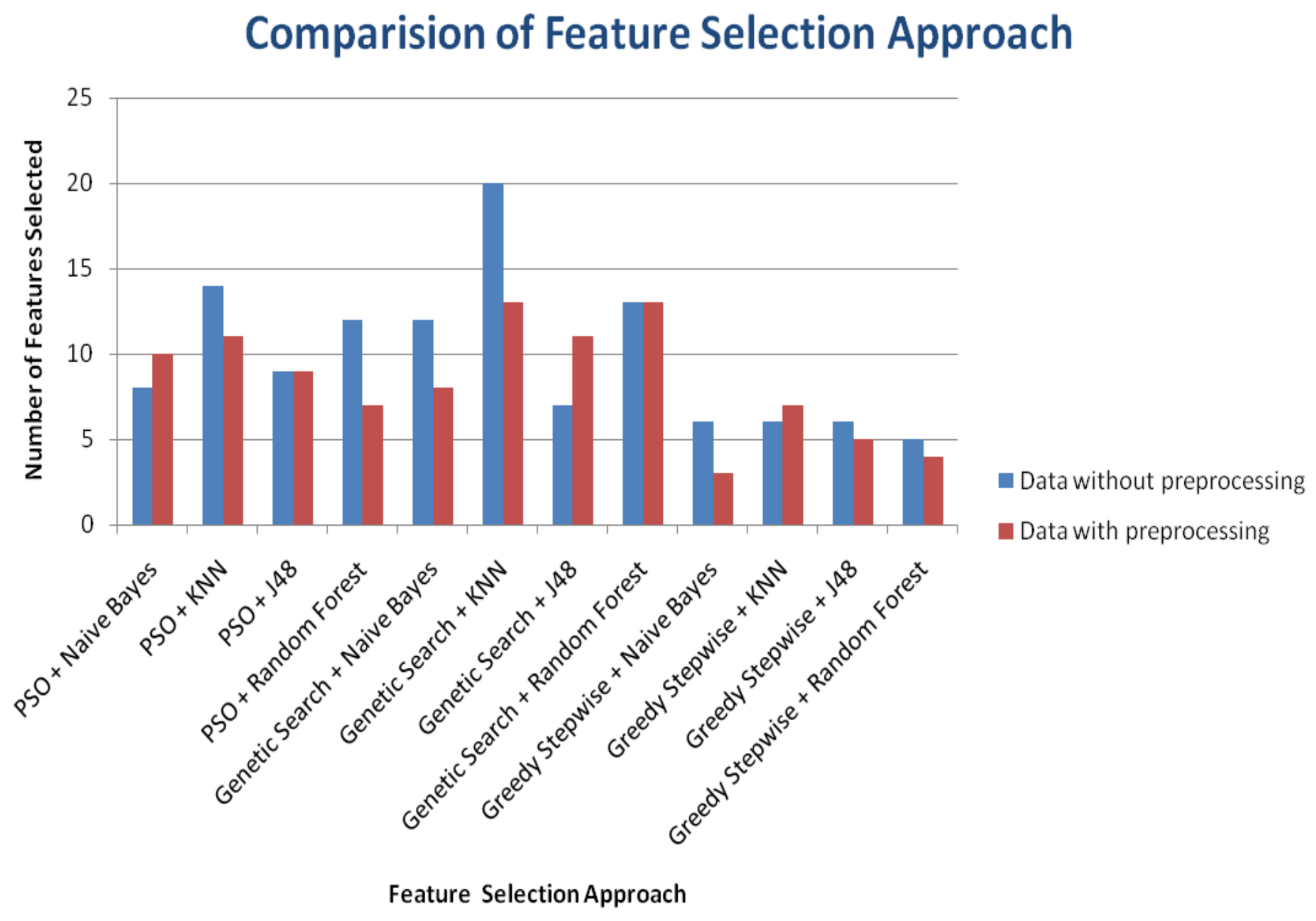
| Classifiers | Wrapper Based Feature Selection Approach | Number of FeaturesSelected | Accuracy(%) | Time to Build the Model (Seconds) | |||
|---|---|---|---|---|---|---|---|
| WoDP | WDP | WoDP | WDP | WoDP | WDP | ||
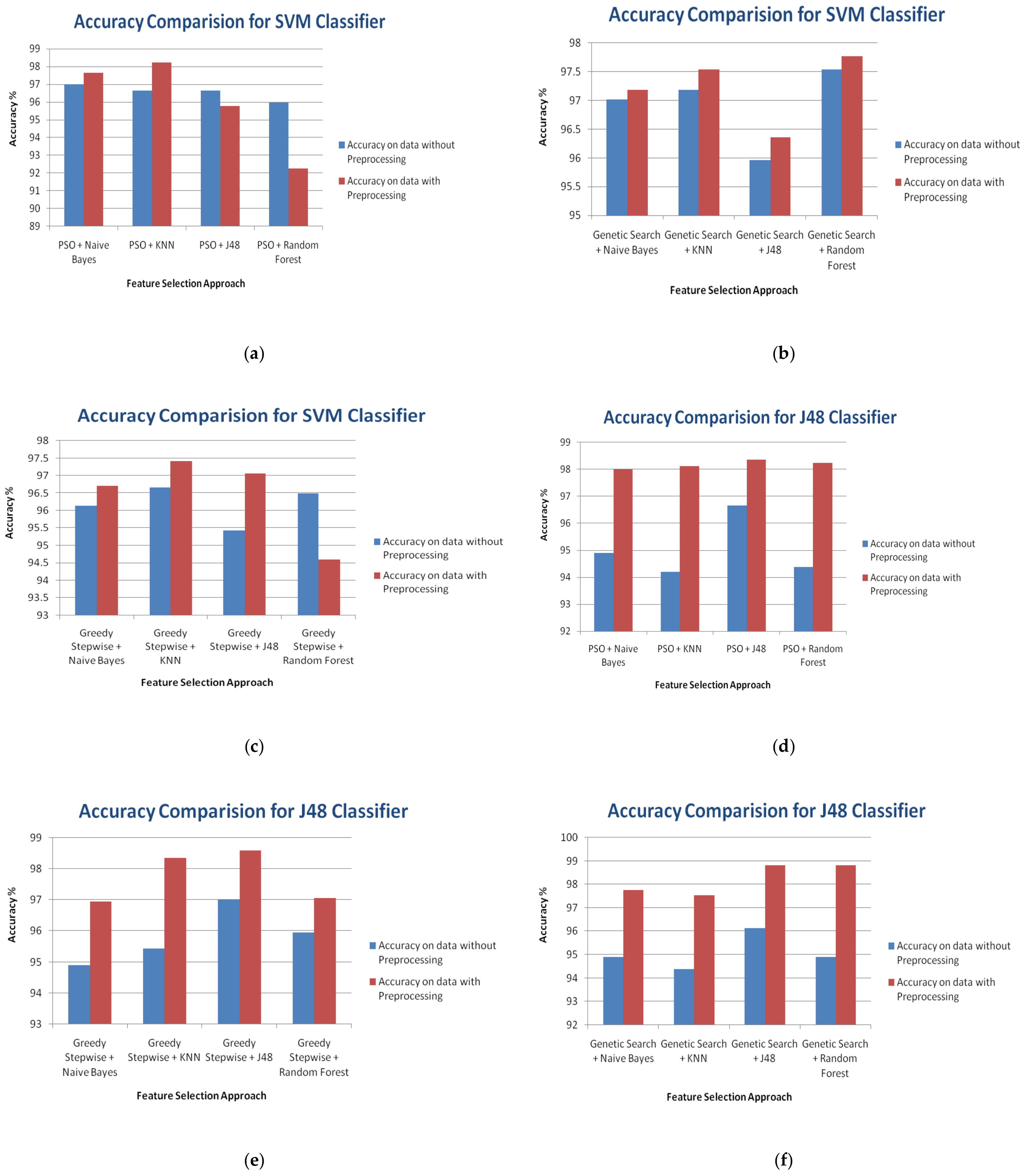
| SVM | PSO + Naive Bayes | 8 | 10 | 97.0123 | 97.6526 | 0.16 s | 0.53 s |
| PSO + KNN | 14 | 11 | 96.6608 | 98.2394 | 0.08 s | 0.03 s | |
| PSO + J48 | 9 | 9 | 96.6608 | 95.7746 | 0.02 s | 0.04 s | |
| PSO + RandomForest | 12 | 7 | 95.9578 | 92.2535 | 0.01 s | 0.02 s | |
| J48 | PSO + Naive Bayes | 8 | 10 | 94.9033 | 98.0047 | 0.03 s | 0.03 s |
| PSO + KNN | 14 | 11 | 94.2004 | 98.1221 | 0.01 s | 0.02 s | |
| PSO + J48 | 9 | 9 | 96.6608 | 98.3568 | 0.01 s | 0.02 s | |
| PSO + RandomForest | 12 | 7 | 94.3761 | 98.2394 | 0.01 s | 0.03 s | |
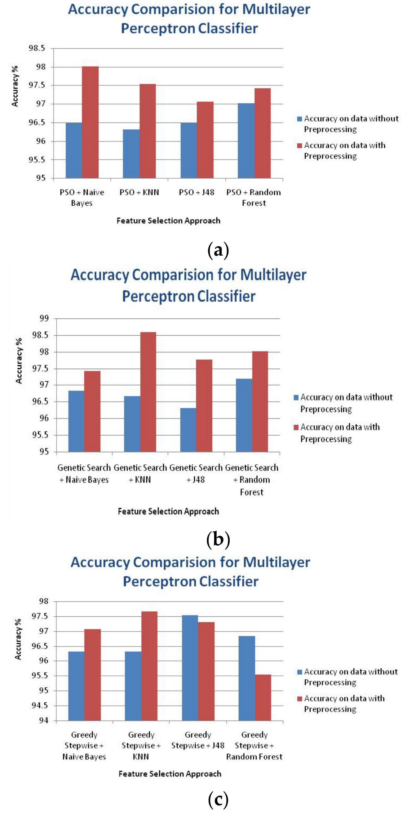
| Multi-Layer Perceptron | PSO + Naive Bayes | 8 | 10 | 96.4851 | 98.0047 | 0.65 s | 0.95 s |
| PSO + KNN | 14 | 11 | 96.3093 | 97.5352 | 1.00 s | 0.98 s | |
| PSO + J48 | 9 | 9 | 96.4851 | 97.0657 | 0.52 s | 0.74 s | |
| PSO + Random Forest | 12 | 7 | 97.0123 | 97.4178 | 0.79 s | 0.60 s | |
| Classifiers | Wrapper Based Feature Selection Approach | Number of Features Selected | Accuracy (%) | Time to Build the Model (Seconds) | |||
|---|---|---|---|---|---|---|---|
| WoDP | WDP | WoDP | WDP | WoDP | WDP | ||
| SVM | PSO + Naive Bayes | 12 | 8 | 97.0123 | 97.1831 | 0.02 s | 0.02 s |
| PSO + KNN | 20 | 13 | 97.188 | 97.5352 | 0.03 s | 0.02 s | |
| PSO + J48 | 7 | 11 | 95.9578 | 96.3615 | 0.02 s | 0.02 s | |
| PSO + Random Forest | 13 | 13 | 97.5395 | 97.7700 | 0.01 s | 0.02 s | |
| J48 | PSO + Naive Bayes | 12 | 8 | 94.9033 | 97.7700 | 0.01 s | 0.01 s |
| PSO + KNN | 20 | 13 | 94.3761 | 97.5352 | 0.02 s | 0.02 s | |
| PSO + J48 | 7 | 11 | 96.1336 | 98.8263 | 0.01 s | 0.01 s | |
| PSO + Random Forest | 13 | 13 | 94.9033 | 98.8263 | 0.01 s | 0.02 s | |
| Multi-Layer Perceptron | PSO + Naive Bayes | 12 | 8 | 96.8366 | 97.4178 | 0.79 s | 0.72 s |
| PSO + KNN | 20 | 13 | 96.6608 | 98.5915 | 1.63 s | 1.23 s | |
| PSO + J48 | 7 | 11 | 96.3093 | 97.7700 | 0.39 s | 1.05 s | |
| PSO + Random Forest | 13 | 13 | 97.188 | 98.0047 | 0.83 s | 1.23 s | |
| Classifiers | Wrapper Based Feature Selection Approach | Number of Features Selected | Accuracy (%) | Time to Build the Model (Seconds) | |||
|---|---|---|---|---|---|---|---|
| WoDP | WDP | WoDP | WDP | WoDP | WDP | ||
| SVM | PSO + Naive Bayes | 6 | 3 | 96.1336 | 96.7136 | 0.01 s | 0.01 s |
| PSO + KNN | 6 | 7 | 96.6608 | 97.4178 | 0.01 s | 0.03 s | |
| PSO + J48 | 6 | 5 | 95.4306 | 97.0657 | 0.02 s | 0.03 s | |
| PSO + Random Forest | 5 | 4 | 96.4851 | 94.6009 | 0.02 s | 0.02 s | |
| J48 | PSO + Naive Bayes | 6 | 3 | 94.9033 | 96.9484 | 0.01 s | 0.05 s |
| PSO + KNN | 6 | 7 | 95.4306 | 98.3568 | 0.01 s | 0.01 s | |
| PSO + J48 | 6 | 5 | 97.0123 | 98.5915 | 0.01 s | 0.01 s | |
| PSO + Random Forest | 5 | 4 | 95.9578 | 97.0657 | 0.01 s | 0.01 s | |
| Multi-Layer Perceptron | PSO + Naive Bayes | 6 | 3 | 96.3093 | 97.0657 | 0.37 s | 0.27 s |
| PSO + KNN | 6 | 7 | 96.3093 | 97.6526 | 0.39 s | 0.58 s | |
| PSO + J48 | 6 | 5 | 97.5395 | 97.3005 | 0.37 s | 0.42 s | |
| PSO + Random Forest | 5 | 4 | 96.8366 | 95.5399 | 0.32 s | 0.40 s | |
| FeatureSelectionApproach | Classifiers | CorrectlyClassifiedInstances (Total 852) | Accuracy (%) | MCC | Sensitivity (%) | Specificity (%) | AUC | PRC Area | Kappa Statistic | Meanabsolute Error | Root Meansquared Error | Relativeabsolute Error (%) | Root Relativesquared Error (%) |
|---|---|---|---|---|---|---|---|---|---|---|---|---|---|
| PSO + Naive Bayes | SVM | 832 | 97.7 | 0.95 | 98.8 | 95.5 | 0.98 | 0.97 | 0.95 | 0.02 | 0.15 | 5.3 | 32.5 |
| J48 | 835 | 98.0 | 0.96 | 98.4 | 97.2 | 0.97 | 0.96 | 0.96 | 0.03 | 0.14 | 5.7 | 29.9 | |
| MP | 835 | 98.0 | 0.96 | 98.9 | 96.2 | 1.00 | 1.00 | 0.96 | 0.03 | 0.13 | 6.2 | 27.1 | |
| PSO + KNN | SVM | 837 | 98.2 | 0.96 | 99.1 | 96.5 | 0.98 | 0.98 | 0.96 | 0.02 | 0.13 | 4.0 | 28.1 |
| J48 | 836 | 98.1 | 0.96 | 98.4 | 97.5 | 0.98 | 0.97 | 0.96 | 0.02 | 0.14 | 5.1 | 28.9 | |
| MP | 831 | 97.5 | 0.95 | 98.2 | 96.1 | 0.99 | 0.99 | 0.94 | 0.03 | 0.14 | 5.9 | 29.6 | |
| PSO + J48 | SVM | 816 | 95.8 | 0.91 | 98.4 | 91.1 | 0.96 | 0.94 | 0.91 | 0.04 | 0.21 | 9.5 | 43.6 |
| J48 | 838 | 98.4 | 0.96 | 98.3 | 98.6 | 0.98 | 0.98 | 0.96 | 0.03 | 0.13 | 5.7 | 26.8 | |
| MP | 827 | 97.1 | 0.93 | 97.5 | 96.1 | 0.99 | 0.99 | 0.93 | 0.04 | 0.16 | 8.4 | 34.6 | |
| PSO + Random Forest | SVM | 786 | 92.3 | 0.83 | 96.1 | 85.4 | 0.92 | 0.90 | 0.83 | 0.08 | 0.28 | 17.4 | 59.0 |
| J48 | 837 | 98.2 | 0.96 | 98.4 | 97.9 | 0.98 | 0.98 | 0.96 | 0.02 | 0.13 | 5.3 | 28.1 | |
| MP | 830 | 97.4 | 0.94 | 98.6 | 95.2 | 1.00 | 1.00 | 0.94 | 0.04 | 0.14 | 8.3 | 29.5 | |
| Genetic Search + Naive Bayes | SVM | 828 | 97.2 | 0.94 | 97.4 | 96.8 | 0.97 | 0.96 | 0.94 | 0.03 | 0.17 | 6.3 | 35.6 |
| J48 | 833 | 97.8 | 0.95 | 98.2 | 96.8 | 0.98 | 0.98 | 0.95 | 0.02 | 0.14 | 5.6 | 30.5 | |
| MP | 830 | 97.4 | 0.94 | 98.8 | 94.9 | 0.99 | 0.99 | 0.94 | 0.03 | 0.14 | 7.8 | 30.0 | |
| Genetic Search + KNN | SVM | 831 | 97.5 | 0.95 | 98.8 | 95.2 | 0.98 | 0.97 | 0.94 | 0.02 | 0.16 | 5.5 | 33.3 |
| J48 | 831 | 97.5 | 0.94 | 97.7 | 97.1 | 0.97 | 0.97 | 0.94 | 0.03 | 0.15 | 6.1 | 32.8 | |
| MP | 840 | 98.6 | 0.97 | 98.6 | 98.6 | 0.99 | 0.99 | 0.97 | 0.02 | 0.12 | 4.4 | 25.0 | |
| Genetic Search + J48 | SVM | 821 | 96.4 | 0.92 | 97.4 | 94.4 | 0.96 | 0.95 | 0.92 | 0.04 | 0.19 | 8.2 | 40.5 |
| J48 | 842 | 98.8 | 0.97 | 98.9 | 98.6 | 0.98 | 0.98 | 0.97 | 0.02 | 0.11 | 3.8 | 22.8 | |
| MP | 833 | 97.8 | 0.95 | 97.7 | 97.8 | 1.00 | 1.00 | 0.95 | 0.03 | 0.14 | 6.1 | 29.7 | |
| Genetic Search + Random Forest | SVM | 833 | 97.8 | 0.95 | 98.9 | 95.5 | 0.98 | 0.97 | 0.95 | 0.02 | 0.15 | 5.0 | 31.7 |
| J48 | 842 | 98.8 | 0.97 | 99.1 | 98.2 | 0.98 | 0.98 | 0.97 | 0.02 | 0.11 | 4.0 | 22.9 | |
| MP | 835 | 98.0 | 0.96 | 99.1 | 95.9 | 1.00 | 1.00 | 0.96 | 0.02 | 0.12 | 4.8 | 25.6 | |
| Greedy Stepwise + Naive Bayes | SVM | 824 | 96.7 | 0.93 | 96.9 | 96.4 | 0.96 | 0.95 | 0.93 | 0.03 | 0.18 | 7.4 | 38.5 |
| J48 | 826 | 96.9 | 0.93 | 97.2 | 96.4 | 0.98 | 0.98 | 0.93 | 0.04 | 0.17 | 8.3 | 36.0 | |
| MP | 827 | 97.1 | 0.93 | 97.9 | 95.4 | 1.00 | 1.00 | 0.93 | 0.04 | 0.14 | 8.9 | 30.7 | |
| Greedy Stepwise + KNN | SVM | 830 | 97.4 | 0.94 | 97.4 | 97.5 | 0.97 | 0.96 | 0.94 | 0.03 | 0.16 | 5.8 | 34.1 |
| J48 | 838 | 98.4 | 0.96 | 98.8 | 97.5 | 0.98 | 0.98 | 0.96 | 0.02 | 0.13 | 4.7 | 27.0 | |
| MP | 832 | 97.7 | 0.95 | 98.4 | 96.2 | 0.99 | 0.99 | 0.95 | 0.03 | 0.14 | 7.6 | 30.1 | |
| Greedy Stepwise + J48 | SVM | 827 | 97.1 | 0.93 | 98.1 | 95.1 | 0.97 | 0.96 | 0.93 | 0.03 | 0.17 | 6.6 | 36.3 |
| J48 | 840 | 98.6 | 0.97 | 99.1 | 97.6 | 0.99 | 0.98 | 0.97 | 0.02 | 0.12 | 3.6 | 24.8 | |
| MP | 829 | 97.3 | 0.94 | 98.6 | 94.8 | 1.00 | 1.00 | 0.94 | 0.04 | 0.14 | 8.6 | 30.4 | |
| Greedy Stepwise + Random Forest | SVM | 806 | 94.6 | 0.88 | 96.4 | 91.0 | 0.94 | 0.92 | 0.88 | 0.05 | 0.23 | 12.1 | 49.3 |
| J48 | 827 | 97.1 | 0.93 | 97.9 | 95.4 | 0.97 | 0.97 | 0.93 | 0.03 | 0.17 | 7.7 | 35.5 | |
| MP | 814 | 95.5 | 0.90 | 98.0 | 91.0 | 0.99 | 0.99 | 0.90 | 0.07 | 0.18 | 14.8 | 38.7 |
Publisher’s Note: MDPI stays neutral with regard to jurisdictional claims in published maps and institutional affiliations. |
© 2021 by the authors. Licensee MDPI, Basel, Switzerland. This article is an open access article distributed under the terms and conditions of the Creative Commons Attribution (CC BY) license (http://creativecommons.org/licenses/by/4.0/).
Share and Cite
Solanki, Y.S.; Chakrabarti, P.; Jasinski, M.; Leonowicz, Z.; Bolshev, V.; Vinogradov, A.; Jasinska, E.; Gono, R.; Nami, M. A Hybrid Supervised Machine Learning Classifier System for Breast Cancer Prognosis Using Feature Selection and Data Imbalance Handling Approaches. Electronics 2021, 10, 699. https://doi.org/10.3390/electronics10060699
Solanki YS, Chakrabarti P, Jasinski M, Leonowicz Z, Bolshev V, Vinogradov A, Jasinska E, Gono R, Nami M. A Hybrid Supervised Machine Learning Classifier System for Breast Cancer Prognosis Using Feature Selection and Data Imbalance Handling Approaches. Electronics. 2021; 10(6):699. https://doi.org/10.3390/electronics10060699
Chicago/Turabian StyleSolanki, Yogendra Singh, Prasun Chakrabarti, Michal Jasinski, Zbigniew Leonowicz, Vadim Bolshev, Alexander Vinogradov, Elzbieta Jasinska, Radomir Gono, and Mohammad Nami. 2021. "A Hybrid Supervised Machine Learning Classifier System for Breast Cancer Prognosis Using Feature Selection and Data Imbalance Handling Approaches" Electronics 10, no. 6: 699. https://doi.org/10.3390/electronics10060699
APA StyleSolanki, Y. S., Chakrabarti, P., Jasinski, M., Leonowicz, Z., Bolshev, V., Vinogradov, A., Jasinska, E., Gono, R., & Nami, M. (2021). A Hybrid Supervised Machine Learning Classifier System for Breast Cancer Prognosis Using Feature Selection and Data Imbalance Handling Approaches. Electronics, 10(6), 699. https://doi.org/10.3390/electronics10060699