Abstract
As demand for bicycles increases, bicycle-related accidents are on the rise. There are many items such as helmets and racing suits for bicycles, but many people do not wear helmets even if they are the most basic safety protection. To protect the rider from accidents, technology is needed to measure the rider’s motion condition in real time, determine whether an accident has occurred, and cope with the accident. This paper describes an artificial intelligence airbag. The artificial intelligence airbag is a system that measures real-time motion conditions of a bicycle rider using a six-axis sensor and judges accidents with artificial intelligence to prevent neck injuries. The MPU 6050 is used to understand changes in the rider’s movement in normal and accident conditions. The angle is determined by using the measured data and artificial intelligence to determine whether an accident happened or not by analyzing acceleration and angle. In this paper, similar methods of artificial intelligence (NN, PNN, CNN, PNN-CNN) to are compared to the orthogonal convolutional neural network (O-CNN) method in terms of the performance of judgment accuracy for accident situations. The artificial neural networks were applied to the airbag system and verified the reliability and judgment in advance.
1. Introduction
Recently, personal means of transportation, such as kick scooters and Segways, have been gaining popularity. Among them, the demand for bicycles has increased, especially with various delivery services and express delivery businesses. Because of this, many bicycle-related accidents occur every year. This is also seen in traffic accident analysis system (TAAS) statistics. In 2019, there were about 8060 cases of bicycle accidents [1,2,3]. In the case of electric bicycles, performance is regulated, and the speed limit is 32 km/h in the US and 25 km/h in the EU and China [4].
There are many items such as helmets and racing suits for bicycles, but many people do not wear helmets even if they are the most basic safety protection. Because the helmet only protects the head, the rider’s body is exposed to shock in the event of a bicycle accident, and even if an accident is less severe than a car accident, the injury level can be quite serious [5]. Head and neck injuries are directly related to death. In [6], head injuries were found to account for one-third of emergency room visits and three-quarters of deaths in bicycle accidents. To protect the rider from accidents, technology is needed to measure the rider’s motion condition in real time, determine whether an accident has occurred, and cope with the accident.
Human behavioral recognition technology is receiving constant attention [7,8,9,10,11,12,13]. The studies on human behavioral recognition technology mainly use acceleration and angular speed sensors, and vision techniques using images and sound are also mainly used. Recent studies on the recognition of human behaviors such as falling or tripping show an accuracy of about 90%. In [7,8], the situation is recognized through images and videos using a 3D range image sensor or Kinect. However, there are difficulties due to distance and viewing angle when using the image sensor or Kinect. In [9,10,11,12], the motion was measured using a three-axis acceleration and tilt sensor, and the threshold method was mainly used. In [13], shows real and simulated motorcycle fall accidents are analyzed. It takes 0.1 to 0.9 s to reach the ground after an accident. In particular, behavioral recognition technology is applied to personal portable devices and game equipment to provide various contents. There are also studies on postural prediction and accident prevention using EMG sensors and artificial intelligence [14,15,16,17,18,19,20]. In [14], motion is detected through an artificial neural network by measuring the movement of a human leg. In [15], a real-time safety monitoring vision system using four image sensors is presented, and behaviors are inferred by fusion with CNN and CSS-PI modules. In [16,17], motion is recognized on the basis of a smartphone, and an electronic compass and three-axis accelerometer are used. In [18,19,20], movement is distinguished using IMU or electromyography and combined with machine learning.
This paper describes an artificial intelligence airbag for bicycles. The artificial intelligence airbag is a system that measures real-time motion conditions of a bicycle rider using a six-axis sensor and judges accidents with artificial intelligence to prevent neck injuries. The composition of this paper is as follows: Section 2 introduces the entire system, and Section 3 explains the comparison and analysis of experimental data. Section 4 describes the structure of the artificial neural network designed in this paper. Section 5 shows the results of testing the model made from the designed artificial neural network. Finally, Section 6 presents a conclusion by summarizing the results of this paper.
2. Safety Airbag System Design
This system is an airbag system that prevents injury to the rider’s neck in the event of a bicycle accident. In this system, the sensor measures the rider’s acceleration and angular velocity conditions, and based on the figures, artificial intelligence detects an accident and operates the airbag.
An MPU 6050 sensor is used to measure acceleration and angular velocity, and the system is composed of a Raspberry Pi 3B for whole system operation and artificial intelligence, an airbag drive circuit for signaling, and an explosion section.
2.1. Sensing Part Design
The MPU 6050 is used to identify changes in the rider’s movement during normal and accident conditions. In the comparison of the data obtained by measuring the acceleration and angular velocity of each of the three axes from the MPU 6050, the waveform has its own characteristics depending on the rider’s movement [1,2,3].
Using the similarity of the waveforms on each axis, artificial intelligence was used to determine whether bicycle accidents happened or not. The MPU 6050′s acceleration and angular velocity have three axes, namely the X, Y, and Z axes, and the directions of the axes are shown in Figure 1.
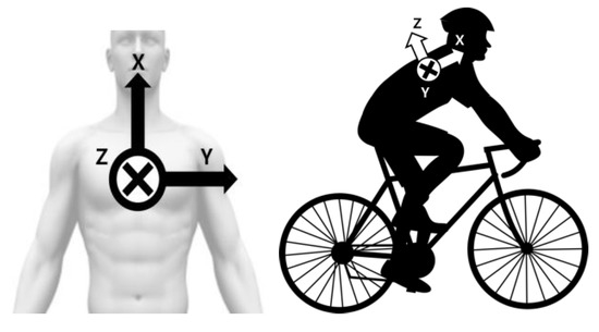
Figure 1.
Axis reference seen from front and left.
In this experiment, a complementary filter and a moving average filter were used to compensate for the unstable values of each axis [21].
The three acceleration axes are , , and , and the sums of the 10 most recent sampling values for each axis are , , and . Here, the equation with the moving average filter is the same as (1)–(4). As a result, this equation reduces the error of acceleration and sensor noise [1,2,3].
The complementary filter is used to calculate the angle relative to the opposite axis of gravity, depending on the stopping or driving conditions. Because the complementary filter’s calculation method depends on the rider’s condition, the problem of cumulative errors from the integration continued is prevented. The complementary filter’s equations are (5) and (6). In the equations, is the complemented angle, is the angle calculated using the angular velocity, and is the angle calculated using the acceleration [22].
The x and y values are continuously adjusted depending on the importance of and when calculating the angle. If the total acceleration received by the sensor (all three accelerations combined) is close to 1G, the y value increases, and in the opposite case, the x value increases. Therefore, the accumulation of errors over time is prevented, and in case of sudden rotation or collision, the angle is tracked around the angular velocity, so it is possible to react quickly. The data are stored in the SD card as a CSV file.
2.2. Drive Part Design
The drive section is divided into the circuit part and the explosion part. The Raspberry Pi 3B in the circuit part operates the entire system, and the PCB circuit board is equipped with a sensor, a motor driver, and a DC–DC converter. The explosion part consists of a choke valve, a 12 V DC motor, and a cartridge connected to an airbag. The overall composition is shown in Figure 2 [1,2,3].
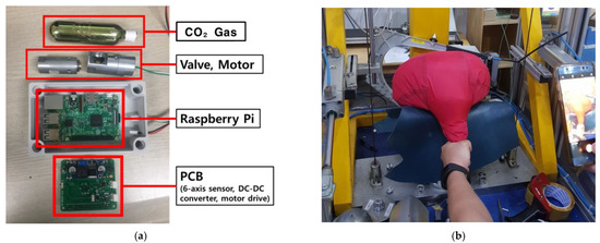
Figure 2.
System configuration: (a) Raspberry Pi 3B, PCB, valve, motor, gas; (b) airbag.
Artificial intelligence in the Raspberry Pi linked with PCB measures the possibility of accidents (Figure 2a). If artificial intelligence detects an accident, the opening of the choke valve causes the cartridge to emit gas, and this leads to bursting the airbag shown (Figure 2b).
It takes about 770 ms for a person to fall in the event of an accident. Since the case of a bicycle accident is faster, the airbag must be inflated in time [14,23]. Thus, the whole system process from the determination of an accident by artificial intelligence to completion of the airbag operation was designed to be shorter than 770 ms. The whole algorithm is shown in Figure 3.
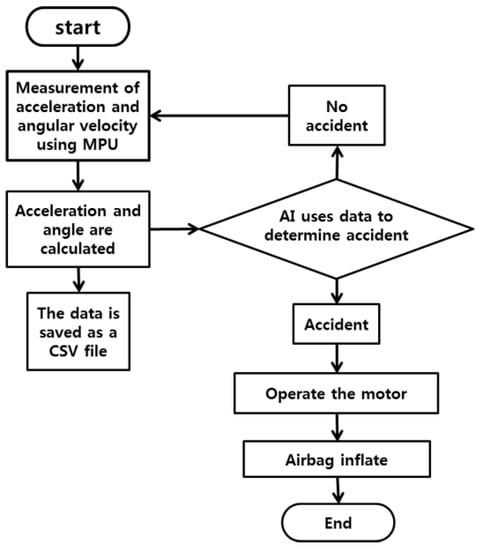
Figure 3.
Safety airbag system algorithm.
3. Data Collection and Analysis
Training data are needed to train artificial intelligence. Training data on characteristics of acceleration and angular velocity depending on a rider’s motion were accumulated through several accident experiments to train artificial intelligence.
3.1. Implementing Accident Situation and Collecting Data
For hypothetical accident simulations, the situations of a frontal impact, a rear impact, a left impact, and a right impact were assumed. The sensor attached to the back of the mannequin measured the mannequin’s motion every 50 ms, and data were stored on the SD card. When collecting data, the data sampled at 50 ms cycle were saved as a CSV file using the MPU 6050 sensor module and Arduino. After the system was configured, additional data were collected with the Raspberry Pi using the same sensor module. When collecting accident data, a mannequin was mounted on a bicycle (with sandbags to increase weight) and crashed while the bicycle was running for an accident situation. The mannequins and the experimental images are shown in Figure 4.
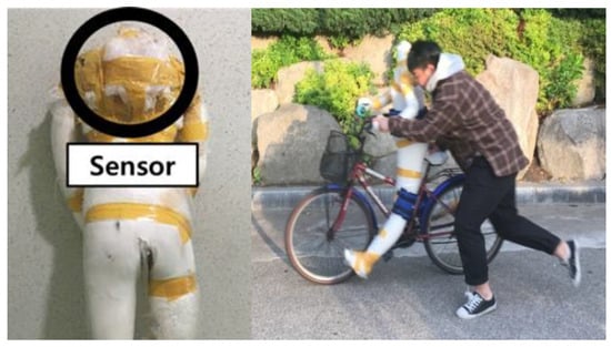
Figure 4.
Mannequin Experiment.
Five situations including front, rear, left, and right impacted situations were tested 20 times. The data for artificial intelligence learning were collected by organizing the acceleration for X, Y, and Z axes, total acceleration value, and angular value for X, Y, and X axes in 50 ms units.
In daily life, people take various positions such as leaning, twisting, and tilting their bodies. To prevent malfunctions in these cases, data on stretching and light movements such as those shown in Figure 5 were additionally obtained. The daily movement data were used as “no accident” data as opposed to accident data when learning [1,2,3].
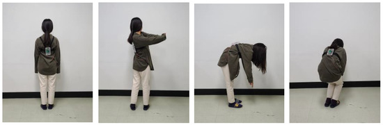
Figure 5.
Stretching and light movements.
3.2. Implementing Accident Situation and Collecting Data
The graphical representation of data obtained from an accident experiment is shown in Figure 6. Figure 6a shows graphs when driving safely; Figure 6b shows graphs when accidents occur. In Figure 6a, the acceleration or angular velocity axis proceeds without significant fluctuation, but in Figure 6b, the acceleration and angular velocity axes fluctuate greatly.
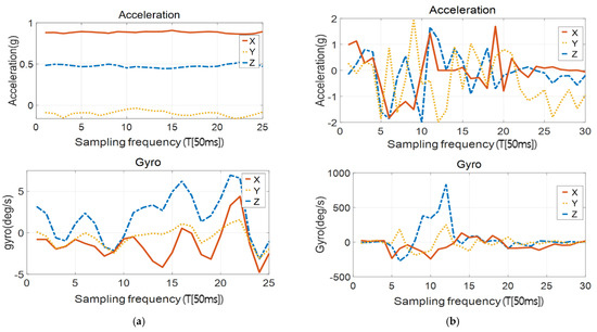
Figure 6.
Accident and no accident graphs: (a) no accident graph; (b) accident graph.
As initial data values had low accuracy due to noise, the raw data were corrected using the moving average filter and the complementary filter mentioned in Section 2.1. The graph of the calibrated data is shown in Figure 7.
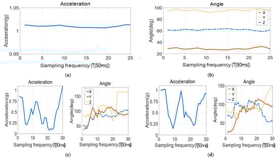
Figure 7.
Corrected acceleration and angle graphs for the cases of no accident and accident: (a) no accident—acceleration; (b) no accident—angle; (c) accident—1; (d) accident—2.
The graphs in Figure 7 show the acceleration and angle of normal driving and accident situations. The graphs in Figure 7a,b are graphs of a normal driving situation; the graphs in Figure 7c,d are graphs of accident situations. The graph in Figure 7a showing the sum of the three-axis acceleration during normal driving shows no significant fluctuation in the acceleration segment. The graph in Figure 7b showing the angle of each axis during normal driving shows a constant angle. The left graphs Figure 7c,d show the acceleration in the event of an accident, and the right graphs show the angle of each axis in the event of an accident. All of these graphs show that the values change rapidly at a particular point, unlike the graphs in Figure 7a,b. The graphs in Figure 7c,d depict experimental data obtained by testing the same accident type. Comparing them to each other shows that the data present a similar waveform in the same accident type. Using the data obtained in the experiment, a dataset was created to train artificial intelligence [1,2,3]. By cutting the accident data from the section before the rider impact and using it for training, we secured enough time for the airbag to inflate.
Figure 8 is a screenshot of how the filtered input data appear when the AI model receives input from the Raspberry Pi in real time. From the left, the values respectively mean the sampling time, acceleration, and angle. As there are three axes of acceleration and angle, the values for acceleration and angle are arranged by three each in the order of XYZ.
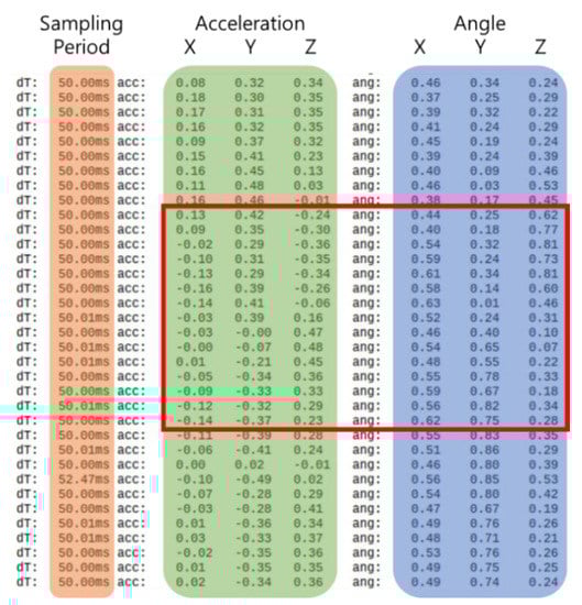
Figure 8.
Screenshot of the input data.
The 90 values in the box are input at the same time. Among the five ANNs that are explained in the following sections, there are the ANNs whose input layer is the convolution layer. The AI model made by these used the input form of the 6 × 15 matrix. The rest of the AI models used the input form of the 90 arrays.
4. Orthogonal Convolutional Neural Network (O-CNN) Design
In this paper, the artificial neural network was designed using the web application “Jupyter Notebook” and Google’s machine learning library “TensorFlow”. A more complex classification should be possible because the type of accidents and the drastic movements that are not accidents are included as learning data. Therefore, ANN was used instead of SVM. The artificial neural network has two convolution layers. The two convolution layers have completely different types of filters. These two layers were used in parallel in the same input layer. In this paper, the artificial neural network designed based on the above method is defined as an orthogonal convolutional neural network (O-CNN). A simple illustration of the O-CNN is shown in Figure 9.
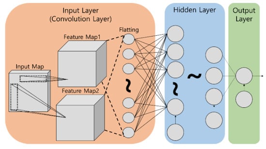
Figure 9.
O-CNN design.
The input of O-CNN is the data consisting of acceleration and angle. Acceleration is the value obtained by applying the moving average filter to the raw acceleration data of MPU 6050 for bias correction. The angle is the value measured by applying the complementary filter to the acceleration and angular velocity values. The filtered acceleration and angle data were used to train the artificial neural network by supervised learning. The acceleration and angle data both have X, Y, and Z axes. Thus, the input data have six types of data. To put the input map into the conversion layer, the data must take the form of a matrix. Thus, in this paper, input data were converted into the form of a matrix based on data type and time.
Because the artificial neural network must react within the time it takes a person to fall (770 ms), the time range for the input data was set at 750 ms [14,19,23]. The sampling interval was fixed at about 50 ms. Therefore, the number of samples in a single input data is 15. The input map of the artificial neural network has a matrix of six data types and 15 sampling steps. As a result, there are 90 values in one input map.
To explain the input map (input of convolution layer), its shape is shown in Figure 10, and it takes the form of a matrix composed of 6 rows and 15 columns. Each of the six rows is classified by data type; the 15 columns represent 15 sampling steps, and each column has six types of data sampled simultaneously. The input map is imported from the training data set stored in an Excel file. Of the values stored in the Excel, the acceleration ranges from −2G to +2G, and angle ranges from −180 to +180°. However, the artificial neural network needs to have a value between −1 and 1 for the input data to benefit from learning. Therefore, the acceleration from the input data was divided by 2 and the angle was divided by 180. In other words, the actual input map consists of values between −1 and 1 [24,25,26,27].
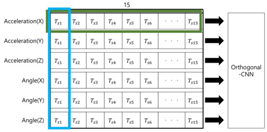
Figure 10.
Input map structure of the artificial neural network.
The O-CNN used two convolution layers for the input layer. Both convolution layers were used only as a single layer at the input layer position. The O-CNN’s convolution layers used four filters each. Each filter on the convolution layer has the form of 1 × 15 and 6 × 1 matrix, which is the same as the green and blue boxes in Figure 10. The filters are used as described above to make 1 × 15 filters analyze changes with time for each type of data and to make 6 × 1 filters analyze the state of data measured at the same sampling time. The activation function ELU is applied to the values obtained through the convolution operation of the filter and the input map. In the convolution operation, the stripe, which means the moving interval of the filter, was 1 × 1. The size of the feature map is set equal to the input map by temporarily adding padding with zero values in the process of the convolution operation. Pooling was not used. In the input layer, a total of eight feature maps created through the above process are transferred to the hidden layer [28,29,30,31,32].
Both the hidden and output layers, except the input layer of O-CNN, are constructed in a fully connected neural network. The activation functions used in the hidden layer are tanh and ELU, and sigmoid is used to distinguish between accidents (1) and no accidents (0) in the output layer. ELU is one of the modified forms of the ReLU activation function, and the equation is as follows:
The activation functions were used in the order of ELU–ELU–tanh–ELU–tanh–sigmoid from the input layer to the output layer [31,32,33,34].
O-CNN performs binary classification of accidents and non-accidents. Because binary classification needs just two classes, such as 0 and 1, the output layer is made into a single node. The number of nodes per layer in the artificial neural network used in this paper is 90 (size of input map)–720–90–30–15–8–1 in sequence from the input layer to the output layer. Figure 11 shows the topology of all artificial neural networks except O-CNN [30,31,32].
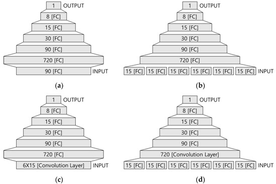
Figure 11.
The topology of artificial neural networks: (a) NN; (b) PNN; (c) CNN; (d) PNN-CNN.
The learning method was supervised learning, and the training data were the experimental data obtained from a result of the experiment described in Section 3. Because supersived learning requires correct answers, accident experimental data and non-accident experimental data were classified in advance to create data sets. The total number of experimental data was 664. The number of non-accident experimental data was 587, and the number of accident experimental data was 77. However, the test data were separated before learning. The setting answer of the artificial neural network for accident experimental data was 1, and the setting answer of the artificial neural network for non-accident experimental data was 0. Inputting the error between the artificial neural network’s output and the correct answer during learning into the loss function provides a scale to determine the learning direction and size of an artificial neural network. In this experiment, cross-entropy (CEE) was used for a loss function. The value of the loss function obtained by CEE was used as an input to the optimization function. The optimization algorithm used adaptive moment estimation (ADAM) optimization techniques. O-CNN was trained under the above process and design [26,27,28,33,34,35].
In addition, dropouts were applied to prevent the overfitting of the artificial neural network. Dropout was set to randomly select 90% of all nodes to be trained. When 90% of the nodes were trained, the remaining 10% were not trained.
5. Artificial Neural Network (ANN) Test Results
We focused on making the ANN lighter and more accurate. In other words, we limited the number of nodes and layers and conducted research to create the best-performing ANN. Through this, we tried to develop an ANN that operates with fast and accurate performance with a small capacity. In this paper, to compare the test results of O-CNN and other neural networks, all conditions of other neural networks, such as the number of layers, number of nodes, and optimization algorithm, were designed to be as similar as possible to O-CNN. The artificial neural networks used for comparison are neural network (NN), parallel neural network (PNN), convolutional neural network (CNN), and parallel neural network–convolutional neural network (PNN-CNN). Except for O-CNN, other neural networks had been applied to the airbag system in previous studies to verify reliability and judgment ability.
Refs. [1,2,3] are the papers in which other ANNs were used in the same system. Ref. [1] explains NN and PNN. Ref. [1] shows PNN is more suitable than NN for the airbag system as PNN has higher accuracy than NN. PNN is similar to NN but uses six parallel layers at the input layer. In Ref. [2], NN, PNN, and CNN are compared. CNN, which uses a convolutional layer at the input layer, showed significantly higher accuracy than NN and PNN. In Ref. [3], PNN, CNN, and PNN-CNN are compared. PNN-CNN uses a parallel layer and a convolutional layer together. The parallel layer is used for the input layer, and the convolutional layer is used for the next layer. PNN-CNN had the highest test accuracy of the three ANNs (PNN, CNN, and PNN-CNN) [1,2,3]. This paper proves that the reliability and judgment ability of O-CNN have been improved compared to the artificial neural networks of [1,2,3]. In the first test, all artificial neural networks were trained 1000 times. The test data were separated from the entire experimental data before the artificial neural network was trained. The test was conducted by comparing and verifying the output from the test data given to the artificial neural network with the correct answers.
Figure 12 is a graph of how the training accuracy and loss function values of the artificial neural networks change during the course. Of the two graphs in Figure 12, the above graph shows the training accuracy, and the graph below shows the loss function values. The horizontal axis of the graph is the number of times and the axis is in order from left to right. However, it indicates the average of the results of 50 tests, not 1. Here, the training accuracy is an indication of the accuracy of how well the artificial neural network fits with the training data, and training accuracy data are different from the test accuracy. The loss function value was obtained by applying cross-entropy (CEE) to the output of the artificial neural networks.
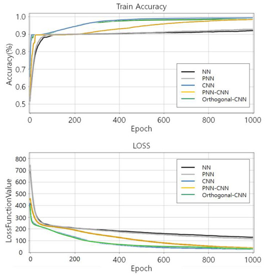
Figure 12.
Comparison of training accuracy and loss function value.
Test performance was verified by inputting test data into the artificial neural networks that completely finished learning. The accuracy of the artificial neural networks test was determined from test results. Table 1 is the actual test result. Table 1 shows eight graphs. These graphs present a total of four data from the test data, two for the accident and two for non-accident. Lines 1 and 2 of Table 1 are test results for non-accident data. Lines 3 and 4 are the results of tests on accident data. In addition, the graph in the “Acceleration” column of Table 1 is a graph of acceleration, and the graph in the “Angle” column shows the angle. In all graphs, the gray solid line is the x-axis, the blue solid line is the y-axis, and the red solid line is the z-axis. In all graphs, the horizontal axis is the sampling sequence, with the left representing the past and the right representing the present. On the right side of the graph is the correct answer to the test data and the value determined by the artificial neural network. The column named “Correct Answer” is a division of the non-accident and the accident state by 0 and 1. The non-accident is 0 and the accident is 1. Artificial intelligence models should export the output close to 0 in the case of non-accident and close to 1 in case of an accident. A standard is needed to calculate the accuracy of how well the judgments fit the correct answers. Based on the criteria established in this paper, an artificial intelligence model must output a value less than 0.5 to fit the correct answer when non-accident data are inputted. On the contrary, an artificial intelligence model must output a value greater than 0.5 to fit the correct answer when the accident data are inputted. Accuracy refers to the percentage of data correctly determined among the total data entered.

Table 1.
Comparison of the results.
The results of NN in Table 1 show that all non-accident cases are correct, but slightly farther from 0 than other artificial neural networks. In the accident cases, one case fits the correct answer by outputting 0.734, but the other case could not fit the correct answer by outputting 0.205. For PNN, the AI model’s output on non-accident cases is a relatively distant value from 0, but all are correct like NN. However, in both cases of accidents, the output values increased and were closer to the correct answer than NN. In one of the two cases, its input was over 0.5 and fit the right answer. Unfortunately, the other case’s output was 0.489 and failed to fit the right answer by a narrow margin. With the introduction of CNN, the artificial intelligence model’s ability to judge non-accident situations was improved, significantly reducing the error. In addition, the ability to judge accident situations was improved significantly, with both outputs for accident data exceeding 0.5 (0.954 and 0.758). This means that the AI model applying CNN can output the correct answer. The AI model introducing PNN-CNN was similar to the AI model applying CNN in non-accident cases. The difference is the ability to judge accident situations. Regarding the same accident data, the AI model applying PNN-CNN had a smaller error (outputting 0.917) than the AI model applying CNN (outputting 0.758). The subject of this paper, O-CNN, showed the highest judgment performance. The AI model applying O-CNN showed the smallest error by outputting 0.009 and 0.006 for non-accident situations and 0.983 and 0.933 for accident situations.
Table 2 shows the training accuracy, test accuracy, training time, and test time of the artificial neural networks used in the experiment. Training accuracy refers to the accuracy of the artificial neural network output for the training data after training 1000 times. Test accuracy refers to the accuracy of how correct the artificial neural network output was regarding the test data when tested as in Table 1 after training 1000 times, the same as for the training accuracy. Training time refers to the average of the time spent on training for each time. The test time refers to the average of the time spent on predicting by putting the test data into the trained AI model and obtaining the output. In every experiment, the AI model was reset and trained 1000 times. Table 2 records the average of 50 experimental results based on this method.
Table 2.
Comparison of artificial neural networks (NN, PNN, CNN, PNN-CNN, O-CNN).
According to the Table 2, CNN has the highest training accuracy, followed by O-CNN, PNN-CNN, PNN, and NN. O-CNN has the highest test accuracy, followed by PNN-CNN, CNN, PNN, and NN. PNN has the shortest training time, and the training time increases in the order of NN, CNN, O-CNN, and PNN-CNN. PNN has the shortest test time, and the test time increase in the order of NN, O-CNN, CNN, and PNN-CNN. Among artificial neural networks with convolutional layers, O-CNN has the shortest test time.
Figure 13 is a receiver operating characteristic (ROC) curve graph. An ROC curve is a graph where the x-axis is false positive rate (FPR) and the y-axis is true positive rate (TPR). TPR is also called sensitivity and it means the rate at which an AI model correctly predicts 1 for answer 1. FPR means the rate at which an AI model wrongly predicts 1 for answer 0. Figure 13 shows the average of 50 experiments as in Figure 12. In regard to the graph’s lines, the black line is for NN, the red line is for PNN, the blue line is for CNN, the yellow line is for PNN-CNN, and the green line is for O-CNN. The area under the ROC curve (AUC) is the area below the ROC curve, and it indicates the suitability of the artificial intelligence method for the target system or data. If the AUC value is 0.5, the ANN model cannot distinguish between positive and negative classes. The closer the AUC value is to 1, the better the distinction between the two classes can be made. In the comparison of AUCs of the artificial neural networks in Figure 13, the AUC values of the ANNs are calculated to be 0.576 for NN, 0.617 for PNN, 0.901 for CNN, 0.958 for PNN-CNN, and 0.984 for O-CNN. That is, O-CNN is the most suitable to make the AI model for bicycle accident judgments.
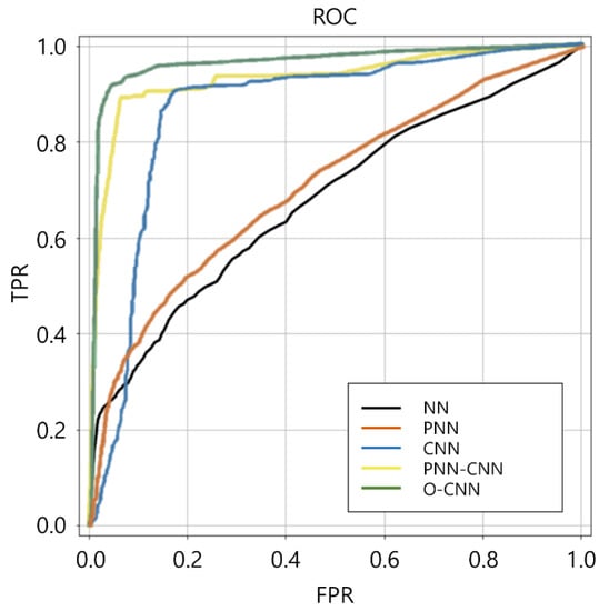
Figure 13.
Comparison of ROC curves (NN, PNN, CNN, PNN-CNN, O-CNN).
6. ANN Comparison and Substantiation
The results of the experiments of O-CNN and four artificial neural networks are compared in Figure 12 and Figure 13 and Table 1 and Table 2 in Section 5. Looking at Figure 12, the graph of NN and PNN shows that the training accuracy is only around 90%. On the other hand, CNN, PNN-CNN, and O-CNN, which have a convolution layer, have a training accuracy of more than 90%. Of these, the training accuracy of PNN-CNN increases slowly, while those of CNN and O-CNN quickly increase, almost at the same level. Therefore, as can be seen from the comparison in Figure 12, O-CNN and CNN have excellent performance in learning the bicycle rider motion data.
Next, a comparison of the accuracy of artificial neural networks is made, as shown in Table 2. Looking at the average values at the bottom of Table 2, PNN is better than NN in all aspects of accuracy. In addition, CNN, PNN-CNN, and O-CNN are generally better than PNN in terms of accuracy. CNN, PNN-CNN, and O-CNN have different rankings for training accuracy and test accuracy. Among the three, CNN has the highest training accuracy and PNN-CNN has the lowest training accuracy. However, in regard to test accuracy, CNN shows the lowest test accuracy while O-CNN has the highest test accuracy. In particular, the difference in training accuracy between CNN and O-CNN is 0.25%. On the other hand, the difference in test accuracy is 1.00%. In other words, O-CNN has the best test accuracy with high training accuracy that is similar to CNN. This means that O-CNN is learning by avoiding overfitting when learning rider motion data more than other artificial neural networks.
Next, a comparison of the speed of the artificial neural networks is made, as shown in Table 2. Like accuracy, average values are compared for speed. PNN is the fastest for both training time and test time. NN shows the shortest training time and test time among the remaining neural networks, except for PNN. Among CNN, PNN-CNN, and O-CNN, PNN-CNN recorded an overwhelmingly slow training time and test time. In particular, PNN-CNN’s test time is longer than 2 ms. Thus, in terms of speed, PNN-CNN has the worst performance. In comparing CNN to O-CNN, the ranking differs for the training time and test time. CNN was faster than O-CNN in training time, and O-CNN was faster than CNN in test time.
After the simulation of the artificial neural networks, the motor train was built as in Figure 14 for the actual test. The performance of O-CNN was verified by reproducing the accident situation after mannequins were seated on the motor train instead of a person. The testbed’s top speed was 50 km/h. However, the top speed of normal electric bicycles is limited to 25 km/h in the EU and China and 32 km/h in the US. Thus, we tested at 30 to 35 km/h [4].
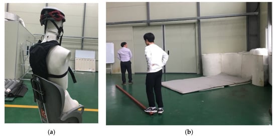
Figure 14.
Testbed: (a) mannequin with experimental equipment; (b) obstacle and mattresses.
To check the performance, artificial intelligence was installed in the Raspberry Pi in the airbag system of the same composition as Figure 14. The airbag was equipped on a mannequin and tested in forward, backward, left, and right directions. The accident situation was tested by directing the motor train to run toward the direction of the raised obstacle spot at high speed and hit the raised obstacle spot. The test results showed that the airbags were activated before touching the floor, as shown in Figure 15, to protect the neck of the mannequin. The time from the train hitting the obstacle to the airbag fully inflating was about 380 ms. For the four side collisions, it was verified that the airbag system operated well between hitting the obstacle and touching the floor.
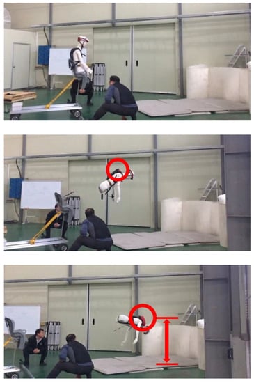
Figure 15.
Airbag drive confirmation.
7. Conclusions
In this paper, O-CNN was proposed as an ANN to be applied to airbag systems to protect the safety of riders using MPU 6050. The whole airbag system was tested by a self-made testbed that ran 30 to 35 km/h. The airbags were fully inflated in about 380 ms before reaching the group. Four ANNs (NN, PNN, CNN, and PNN-CNN) were compared with O-CNN by objective results. O-CNN had the highest test accuracy (97.25%) of the five ANNs. O-CNN had the shortest test time (1.356 ms) of the three ANNs with a convolution layer. Additionally, O-CNN had the widest ROC and the highest AUC value (0.984). For the airbag system, accuracy and reaction speed are the most important indexes. O-CNN passed the real-world test and proved that it fits the airbag system better than other ANNs through various comparisons.
This implementation of the O-CNN was focused on using convolution layers in determining how a rider’s posture and movements change over time. Future studies will focus more on the change over time. In order to do that, future studies will have to study the model of a new ANN.
Since the system uses motors to inflate the airbag, it takes some time (about 220 ms) to receive signals and fully inflate the airbag. Improving these physical elements can reduce the amount of time required, which can enable the inflation of a larger airbag and the more rapid protection of the rider.
Author Contributions
Conceptualization, J.-H.J.; methodology, J.W., B.-S.K., and J.-H.J.; software, J.W.; validation, S.-H.J. and J.-H.J.; formal analysis, J.W.; investigation, S.-H.J. and G.-S.B.; data curation, J.W. and S.-H.J.; writing—original draft preparation, J.W. and S.-H.J.; writing—review and editing, J.W. and S.-H.J.; visualization, J.W. and S.-H.J.; supervision, J.-H.J., B.-S.K., and G.-S.B.; project administration, B.-S.K., J.-H.J., and G.-S.B. All authors have read and agreed to the published version of the manuscript.
Funding
This research was partially supported by the Institute of Information and Telecommunication Technology of KSNU.
Conflicts of Interest
The authors declare no conflict of interest.
References
- Jo, S.H.; Woo, J.; Jeong, J.H.; Byun, G.S. Safety Air Bag System for Motorcycle Using Parallel Neural Networks. J. Electr. Eng. Technol. 2019, 14, 2191–2203. [Google Scholar] [CrossRef]
- Woo, J.; Jo, S.H.; Jeong, J.H.; Kim, M.; Byun, G.S. A Study on Wearable Airbag System Applied with Convolutional Neural Networks for Safety of Motorcycle. J. Electr. Eng. Technol. 2020, 15, 883–897. [Google Scholar] [CrossRef]
- Jeong, J.H.; Jo, S.H.; Woo, J.; Lee, D.H.; Sung, T.K.; Byun, G.S. Parallel Neural Network–Convolutional Neural Networks for Wearable Motorcycle Airbag System. J. Electr. Eng. Technol. 2020, 15, 2721–2734. [Google Scholar] [CrossRef]
- Salmeron-Manzano, E.; Manzano-Agugliaro, F. The electric bicycle: Worldwide research trends. Energies 2018, 11, 1894. [Google Scholar] [CrossRef]
- Quick Service Two Wheeled Vehicle Delivery Safety Guide. 2017. Available online: http://www.kosha.or.kr/kosha/data/business/transpotransp.do?medSeq=37934&codeSeq=1150180&mmedFor=101&menuId=-1150180101&mode=view (accessed on 10 April 2017).
- Thompson, D.C.; Rivara, F.; Thompson, R. Helmets for preventing head and facial injuries in bicyclists. Cochrane Database Syst. Rev. 1999, 97. [Google Scholar] [CrossRef] [PubMed]
- Kawaguchi, S.; Takemura, H.; Mizoguchi, H.; Kusunoki, F.; Egusa, R.; Funaoi, H.; Sugimoto, M. Accuracy evaluation of hand motion measurement using 3D range image sensor. In Proceedings of the Sensing Technology (ICST), 2017 Eleventh International Conference on Sensing Technology (ICST), Sydney, Australia, 4–6 December 2017; pp. 1–4. [Google Scholar]
- Stone, E.E.; Skubic, M. Fall detection in homes of older adults using the Microsoft Kinect. IEEE J. Biomed. Health Inform. 2015, 19, 290–301. [Google Scholar] [CrossRef]
- Ryu, J.T. The development of fall detection system using 3-axis acceleration sensor and tilt sensor. J. Korea Ind. Inf. Syst. Res. 2013, 18, 19–24. [Google Scholar]
- Kim, S.H.; Park, J.; Kim, D.W.; Kim, N. The Study of Realtime Fall Detection System with Accelerometer and Tilt Sensor. J. Korean Soc. Precis. Eng. 2011, 28, 1330–1338. [Google Scholar]
- Kim, H.; Min, J. Implementation of a Motion Capture System using 3-axis Accelerometer. J. Kiise Comput. Pract. Lett. 2011, 17, 383–388. [Google Scholar]
- Lee, S.M.; Jo, H.R.; Yoon, S.M. Machine learning analysis for human behavior recognition based on 3-axis acceleration sensor. J. Korean Inst. Commun. Sci. 2016, 33, 65–70. [Google Scholar] [CrossRef]
- Bellati, A.; Cossalter, V.; Lot, R.; Ambrogi, A. Preliminary investigation on the dynamics of motorcycle fall behavior: Influence of a simple airbag jacket system on rider safety. In Proceeding of 6th International Motorcycle Conference; IFZ Institute for Motorcycle Safety: Cologne, Germany, 2006; pp. 9–10. [Google Scholar]
- Kiguchi, K.; Matsuo, R. Accident prediction based on motion data for perception-assist with a power-assist robot. In Proceedings of the Computational Intelligence (SSCI), 2017 IEEE Symposium Series on Computational Intelligence (SSCI), Honolulu, HI, USA, 27 November–1 December 2017; pp. 1–5. [Google Scholar]
- Ali, Z.; Park, U. Real-time Safety Monitoring Vision System for Linemen in Buckets Using Spatio-temporal Inference. Int. J. Control Autom. Syst. 2020, 19, 505–520. [Google Scholar] [CrossRef]
- Lee, H.; Lee, S. Real-time Activity and Posture Recognition with Combined Acceleration Sensor Data from Smartphone and Wearable Device. J. Kiss Softw. Appl. 2014, 41, 586–597. [Google Scholar]
- Kau, L.J.; Chen, C.S. A smart phone-based pocket fall accident detection, positioning, and rescue system. IEEE J. Biomed. Health Inform. 2015, 19, 44–56. [Google Scholar] [CrossRef]
- Duong, H.T.; Suh, Y.S. A simple smoother for attitude and position estimation using inertial sensor. Int. J. Control Autom. Syst. 2016, 14, 1626–1630. [Google Scholar] [CrossRef]
- Rescio, G.; Leone, A.; Siciliano, P. Supervised machine learning scheme for electromyography-based pre-fall detection system. Expert Syst. Appl. 2018, 100, 95–105. [Google Scholar] [CrossRef]
- Serpen, G.; Khan, R.H. Real-time detection of human falls in progress: Machine learning approach. Procedia Comput. Sci. 2018, 140, 238–247. [Google Scholar] [CrossRef]
- Kim, Y.K.; Park, J.H.; Kwak, H.K.; Park, S.H.; Lee, C.; Lee, J.M. Performance improvement of a pedestrian dead reckoning system using a low cost IMU. J. Inst. Control Robot. Syst. 2013, 19, 569–575. [Google Scholar] [CrossRef][Green Version]
- Yoo, B.H.; Heo, G.Y. Detection of Rotations in Jump Rope using Complementary Filter. J. Korea Inst. Inf. Commun. Eng. 2017, 21, 8–16. [Google Scholar] [CrossRef]
- Zhang, Q.; Li, H.Q.; Ning, Y.K.; Liang, D.; Zhao, G.R. Design and Realization of a Wearable Hip-Airbag System for Fall Protection. Appl. Mech. Mater. 2014, 461, 667–674. [Google Scholar] [CrossRef]
- Sugomori, Y. Detailed Deep Learning-Time Series Data Processing; Keras, T.F., Ed.; Wikibook: Paju-si, Korea, 2017; Chapter 3. [Google Scholar]
- Deep Learning That Literary Students Can Also Understand (2)–Neural Network. Available online: https://sacko.tistory.com/17?category=632408 (accessed on 18 October 2017).
- Kingma, D.P.; Ba, J.L. Adam: A Method for Stochastic Optimization. In Proceedings of the International Conference on Learning Representations, San Diego, CA, USA, 7–9 May 2015; pp. 1–13. [Google Scholar]
- Heusel, M.; Ramsauer, H.; Unterthiner, T.; Nessler, B.; Hochreiter, S. GANs Trained by a Two Time-Scale Update Rule Converge to a Local Nash Equilibrium. In Proceedings of the 31st Conference on Neural Information Processing System, Long Beach, CA, USA, 4–9 December 2017. [Google Scholar]
- Gradient Descent Optimization Algorithms Theorem. Available online: http://shuuki4.github.io/deep%20learning/2016/05/20/Gradient-Descent-Algorithm-Overview.html (accessed on 20 May 2016).
- Li, X.; Ye, M.; Fu, M.; Xu, P.; Li, T. Domain adaption of vehicle detector based on convolutional neural networks. Int. J. Control Autom. Syst. 2015, 13, 1020–1031. [Google Scholar] [CrossRef]
- Lawrence, S.; Giles, C.L.; Tsoi, A.C.; Back, A.D. “Face recognition: A convolutional neural-network approach. IEEE Trans. Neural Netw. 1997, 8, 98–113. [Google Scholar] [CrossRef] [PubMed]
- LeCun, Y.; Bengio, Y. Convolutional networks for images, speech, and time series. Handb. Brain Theory Neural Netw. 1995, 3361, 1995. [Google Scholar]
- Sun, L.; Jia, K.; Yeung, D.Y.; Shi, B.E. Human action recognition using factorized spatio-temporal convolutional networks. In Proceedings of the IEEE International Conference on Computer Vision, Santiago, Chile, 7–13 December 2015; pp. 4597–4605. [Google Scholar]
- Hinton, G.; Srivastava, N.; Swersky, K. Neural networks for machine learning lecture 6a overview of mini-batch gradient descent. 2012. Available online: https://www.cs.toronto.edu/~hinton/coursera/lecture6/lec6.pdf (accessed on 19 April 2021).
- Sutskever, I.; Martens, J.; Dahl, G.; Hinton, G. On the importance of initialization and momentum in deep learning. In Proceedings of the 30th International Conference on Machine Learning (ICML-13), Atlanta, GA, USA, 16–21 June 2013; pp. 1139–1147. [Google Scholar]
- Clevert, D.A.; Unterthiner, T.; Hochreiter, S. Fast and accurate deep network learning by exponential linear units (elus). arXiv 2015, arXiv:1511.07289. [Google Scholar]


Publisher’s Note: MDPI stays neutral with regard to jurisdictional claims in published maps and institutional affiliations. |
© 2021 by the authors. Licensee MDPI, Basel, Switzerland. This article is an open access article distributed under the terms and conditions of the Creative Commons Attribution (CC BY) license (https://creativecommons.org/licenses/by/4.0/).