Abstract
Present-day queuing inventory systems (QIS) do not utilize two multi-server service channels. We proposed two multi-server service channels referred to as (Type 1 n-identical multi-server) and (Type 2 m-identical multi-server). It includes an optional interconnected service connection between and , which has a finite queue of size N. An arriving customer either uses the inventory (basic service or main service) for their demand, whom we call , or simply uses the service only, whom we call . Customer will utilize the server , while customer will utilize the server , and can also get the second optional service after completing their main service. If there is a free server with a positive inventory, there is a chance that customers may go to an infinite orbit whenever they find that either all the servers are busy or no sufficient stock. The orbital customer can request for service under the classical retrial policy. items are replaced into the inventory whenever it falls into the reorder level s such that the inequality always holds . We use the standard ordering policy to replace items into the inventory. By varying S and s, we investigate to find the optimal cost value using stationary probability vector . We used the Neuts Matrix geometric approach to derive the stability condition and steady-state analysis with R-matrix to find . Then, we perform the waiting time analysis for both and customers using Laplace transform technique. Further, we computed the necessary system characteristics and presented sufficient numerical results.
1. Introduction
As we see in real-life scenarios, many motorcycle service centers operate multi-service channels for motorcycle servicing and motorcycle sales. Generally, these services are provided on different floors in the same buildings. Customers, generally, came only for service or buying a bike. However, because the business provides an additional service, the customers who came for motorcycle servicing may go for additional services. In fact, this is not a compulsory service, and it depends on their choice. This situation was impressive and motivated us to make mathematical modeling in a stochastic queuing inventory sector.
In a supply chain’s business operations, the enterprise must update itself in various dimensions to meet its customers’ current requirements and expectations. One of the dimensions of the businesses to keep on updating is through its alternative technologies. The alternative technologies help improving goals that will serve as standards and benchmarks to technically and operationally evaluate its performance. Businesses need to allocate an exceptional value to satisfy the demand for implementing strategic goals. The firm’s focus should aim at a better-spelled strategy to provide efficient and systematic service platforms in their marketing society. Planning well-standard innovative ideas ensures an amalgamation of the demands and retailers more consistently. An ideology of a business requires concentration on making and providing opportunities at every stage.
Most of the firms concentrate on providing an excellent service to their customers by framing new strategies because the overall service-related problems can eventually lead to their name’s demise. When we provide good customer service, they will be more interested in remaining loyal to our business, and this loyalty ensures that they will likely stick around. Looking into the queuing inventory system (QIS), a service facility is essential for all the mechanisms. At the initial time, many researchers discussed the QIS without service facility. When we compare such models to real life, the chances are significantly less to accept the models without a service facility. For example, in modern society, customers are not well aware of the handling procedures and utilizing skills when they wish to purchase their new items. Every customer needs a demonstration while purchasing it. For instance, if a customer wants to buy an induction cooktop, washing machine, refrigerator, etc., they need to know its operating procedure. The system requires the service facility to provide excellent service to their customer. Many authors come forward to attack the QIS with the service facility concerning this. By the way, Melikov and Sigman [1,2] introduced service facilities in their corresponding work, namely the transportation storage system and heuristic queue, respectively.
Berman [3] discussed a deterministic approximation for their inventory system with service facility and found the total cost, which depends upon the average inventory, a customer in the queue, and reorder rates. After some years, Berman [4] studied the same inventory system in which they found an inventory policy that minimizes the total expected customer waiting, ordering, and holding costs over a finite queue and deduces the results to an infinite queue. They also analyzed an optimal order quantity with a simple heuristic method. Berman [5] developed the inventory system with an arbitrary service time for a finite queue. In recent years, Paul Manuel et al. [6] examined a single server inventory system where an arrival follows the Markovian Arrival Process (MAP). Amirthakodi [7] considered an inventory system with a single server service facility and finite retrial feedback customer. For more details about a single server queuing-inventory system, one can refer to References [8,9,10,11,12].
In this emerging society, the single-server system is not convenient for providing a good service. When a new customer enters the waiting hall during the peak hours and sees a long queue in front of them, they get irritated and become impatient, which leads a customer to lose. On behalf of this, Kuo-Hsiung and Keng yuan Tai [13] studied the additional servers that came into the service due to the queue size, which exceeds the threshold level. Jongho Bae [14] introduced an optional service rate named as a two-stage service policy, which means that the server starts work with regular service rate () till the system reaches N customer; after N customer, it turns into a faster service rate , including the customer at the moment. Jeganathan et al. [15] investigated a single server system by varying the speed of service rate under the threshold policy to reduce a customer’s impatience.
However, increasing the server’s speed or providing a faster service rate if the queue length exceeds a fixed limit is not enough to rectify an arriving customer’s impatience, whose expectation is different from this type of service. Jeganathan et al. [16] presented the comparison of homogeneous versus heterogeneous servers in their two-server Markovian inventory system in which they showed an efficiency of a heterogeneous system.
The Markovian inventory scheme with two parallel queues is considered by Jeganathan et al. [17], in which an arriving customer will enter the shortest queue. Meanwhile, we can see in real life that there are two kinds of customers who can approach the system for either service or inventory only. Jeganathan et al. [10] analyze the perishable inventory model of a single server that consists of two priority clients, such as type 1 and type 2. The customer arrival flows are independent Poisson processes, and type 1 and type 2 customer service times are exponential distribution. Pandelis [18] introduced the concept of interconnected queues under different service rates. Apart from the two dedicated servers, they introduced a flexible trained server for working in both stages. The same work has been modeled in a perishable inventory system with two dedicated servers for each service station by Jeganathan et al. [19]. They also assumed a flexible service that can provide the service at any station with a new service rate. Jeganathan and Abdul Reiyas [20] recently researched a modified and delayed working vacation with two priority clients.
Every day-to-day lifestyle requirement changes depending upon time, satisfaction on an item, a fair service process, and so on. Many firms introduced a multi-service channel to reduce customer loss and wait time to satisfy such requirements. According to the inconveniences of a single server queuing model, Krishnamoorthy et al. [21] attempted a parallel server inventory system that consists of a homogeneous service rate. On the other hand, Rajkumar et al. [22] studied an identical server in their inventory system. Arivarignan et al. [23] discussed a multi-server channel in QIS with MAP arrival. Yadavelli et al. [24] gave the extension of work of Arivarignan by introducing negative customers. Nair et al. [25] discussed the multi-server QIS in which a customer leaves the system and the server removed from the system after the service completion. For more details about a multi-server queuing inventory system, refer to References [26,27,28,29,30,31].
The majority of the inventory framework has examined a single type of multi-server with different assumptions from the above discussion. No research has been carried out to the best of our knowledge on combining two multi-server forms in the inventory market. Interestingly, a two multi-server service system in the queuing system is investigated by Cheng-Yuan Ku and Scott Jordan [32]. On doing such keen observation from the literature review, we found and enlisted some research gaps as follows:
- No two multi-server service channels involving QIS.
- Interconnected arrivals between the two multi-server service channels.
- Two different two multi-server service channels providing their service for two different streams of arrival.
Upon a keen survey through the above-mentioned research gaps and motivations, the first time in the QIS, we introduce the interconnected two types of multi-server service channels for providing a satisfactory service of two different arrival streams with which the system allows an optional interconnected arrival between the two multi-service channel.
Customers know that queues are inevitable in many cases. Therefore, the proposed model can satisfy the customer, both in inventory sales and service. This paper preserves the optimum total cost for the interconnected arrival between two multi-server service channel inventory systems. Besides, the probability r (which causes the interconnected arrival between two multi-server service channels) increases, and we achieve a decrement in both customers lost. Further, the waiting time of both retrial and customers’ is derived analytically by Laplace-Stieltjes transform. The numerical analysis results show that it has significant applications in real-life economics.
The rest of the paper is organized as follows. Section 2 describes the proposed model. The analysis of the proposed model is given in Section 3. The waiting time analysis is in Section 4, and system performance measures are detailed in Section 5. The cost analysis and numerical illustration are presented in Section 6, and the conclusion is in Section 7.
2. Model Description
In this section, we describe the proposed model. The notations used in this article are defined in the notation section at the end of the article.
- We study the multi-server perishable queuing inventory system (MPQIS), which comprises two types of multi-server service channels and an interconnected optional arrival between these channels. Type-1 and Type-2 multi-server service channels (T1S and T2S) have n and m number of identical servers, respectively.
- We also allocated both and to be trained servers for dedicated work such that and provide inventory sales and only service (not an item), respectively.
- Customers entering and are named Type-1 and Type-2 customers ( and ), respectively.
- The MPQIS has the accommodation facilities for customer only with a size of N.
- An incoming consumer who learns that either all are busy or not enough stock instantly will enter an orbit with a probability of p or exit the system with a probability of . Here, orbit means that if an arriving customer finds all the servers are occupied, he/she joins a retrial group (virtual waiting place) called an orbit.
- When the time of service completion of customer, they can either claim an additional service with probability r through the waiting hall, called an interconnected (optional) arrival or leave the system with probability .
- A retrial customer can approach the system simultaneously. Still, this approach will succeed only when they know that there exists any free server with ample stock under the classical retrial policy.
- Whenever all the are busy, customer has to wait in the accommodation hall; otherwise, they immediately get their service. Suppose the accommodation hall is full, and they are considered as lost.
- We assume that inventories have the standard of degradation except for items in operation.
- The required replenishment of items will be done whenever S dropped into s under the ordering policy.
- , and retrial arrival process follow independent Poisson distribution. Service of , , reordering, and deteriorating processes follows an exponential distribution.
- The graphical depiction and the model’s transition graph are explained pictorially in Figure 1.
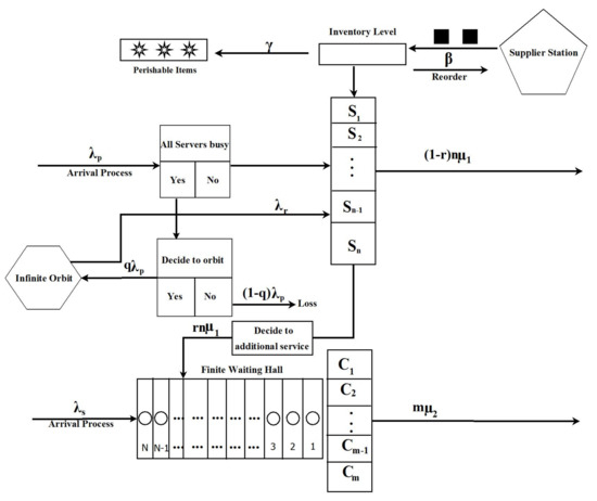 Figure 1. Graphical depiction of the model.
3. Analysis of the Model
The process is a continuous-time Markov chain (CTMC) having the state space E given by .
Define the following ordered sets:
Then, the state space can be ordered as .
Theorem 1.
Referring to the discrete state space with CTMC, the transition of infinitesimal generator matrix of the MPQIS has the structure as follows:
More clearly, the super diagonal matrices of P is given by
The lower diagonal matrices of P is given by
The main diagonal matrices of P is given by:
For
where
For ,
For ,
For ,
For ,
where
For the above matrices , , where are square matrices of order . are square matrices of order . are of order . , are of order , and , , and are square matrices of order .
Proof.
Using the assumption of the proposed model, first, we consider matrix which contains sub-matrices , where , along the diagonal in which entries are the transition rate of customer arrival , enter into an orbit under Bernoulli schedule, we get Equation (2). Next, let us discuss the matrix, where also possesses the sub-matrices , where , along the diagonal, and, again, these sub-matrices, contains another sub-matrix of dimension , in which entries are the transition rate of retrial arrivals based on the classical retrial policy, enter into an orbit, gives the Equation (3). Then, consider the diagonal matrix , where , lower-diagonal of this matrix contains the sub-matrices , where , in which elements are and , which represents the perishable transition rates, which is dependent on the present inventory level and service rate of the customer arrivals, we get the Equations (7) and (8); another sub-matrix is , where , in which entries defined by the rate of reorder transition which follows the ordering policy, using the designed matrix of Equation (6), we construct an Equation (5); finally, the diagonal contains the sub-matrices , where , and it contains the entries Here, is the rate of customer arrival transition enter into the waiting hall, and is the service rate of the customer arrivals, which is dependent on the number of . Then, the diagonal element, filled by the sum of all the entries in the corresponding rows, with a negative sign in order to satisfy the sum of all entries in each row yields zero, and we obtain Equations (9)–(11). Hence, all the sub-matrices obtained through the respective transitions give the infinitesimal generator matrix P, as in Equation (1). □
3.1. Stability Analysis
Let us assume M is the cut-off point of this truncation process for the matrix-geometric approximation. To find the steady-state of the considered system using Neuts-Rao truncation method [33], we assume and for all . Then, the modified generator matrix of the truncated system having the below structure:
Theorem 2.
The steady-state probability vector Φ corresponding to the generator matrix where is given by
where
with
and is obtained by solving
Proof.
The structure of is defined by
where
and the matrices are defined in Equation (4). Let be the steady state probability vector of , and the normalizing condition gives
Then, vector can be represented by Using the equation of , we get the following set of equations:
Theorem 3.
The stability condition of the system at the truncation point M is given by
where
and
Proof.
From the notable result after effect of Neuts [33] on the positive recurrence of , the condition,
provides the result as in (16). □
3.2. Steady State Analysis
It can be seen from the structure of the rate matrix P, and from Theorem 3, that the Markov process with the state space E is regular. Hence, the limiting probability distribution,
exists and is independent of the initial state. Let be the stationary probability vector satisfying
3.3. Computation of R-Matrix
Due to the specific structure of P, using the vector and R can be determined by
where R is the minimal non-negative solution of above matrix quadratic equation, and it is defined by
This R has only non-zero rows of dimension . Now, due to the specified structure of , the structure of the block matrix is of the form:
where
Theorem 4.
The stationary probability vector ϕ of the CTMC can be determined by
where R is a solution of Equation (17) and the vector
where
and can be computed by using the normalizing condition
Proof.
The sub-vector and the block partitioned matrix of gives the set of equations:
using Equation (21),
again, using (21),
where
Next,
where
On continuing this procedure up to times, we get:
where
To find the vectors , we apply block Gaussian elimination method. The sub-vector , corresponding to non-boundary states, satisfies the following relation:
Assume:
From (23), we get
Since =1, then,
Hence,
4. Waiting Time Analysis
The customer wait time () is defined as interim time between an epoch of arrival of a demand enters into the waiting hall or orbit and the instant at which they enter into the service. We examine the of demand in the queue and orbit separately using the Laplace-Stieltjes transform (LST). Naturally, we limit the orbit size to finite for finding the waiting time of an orbital demand. We represent and as the continuous-time random variables to denote the of demand in queue and an orbit. Due to such restriction, the modified state-space of a CTMC is , which is obtained by improving the co-ordinate from to in each
of a Demand in Queue and Orbital Demand
Theorem 5.
The probability of a demand that does not wait into the queue is considered as
where
Proof.
Since the sum of probability of zero and positive waiting time is 1, we have
Clearly, the probability of positive waiting time of demand in the queue can be determined as
To enable distribution of , we shall define some complementary variables. Suppose that the MPQIS is at state at an arbitrary time t:
- is the time until chosen demand become satisfied.
- LST of is , and we denote by .
- LST of unconditional waiting time (UWT).
- LST of conditional waiting time (CWT).
Theorem 6.
The LS transforms {, where satisfy the following system:
, and the matrix J is derived from P by removing the following states and is the absorbing state, and the absorption occurs if the customer demands to enter into the service.
Proof.
To obtain the CWT, we apply first step analysis as follows:
For ,
For ,
where .
For ,
For ,
where .
For ,
For ,
where .
Theorem 7.
The moments of CWT is given by
and
Proof.
On exploring the set of equations which are acquired in Theorem (6), we get a recursive algorithm to find a conditional and unconditional waiting times.
For ,
For ,
where .
For ,
For ,
where .
For ,
For ,
where .
Theorem 8.
The LST of UWT of a demand in the queue is given by
Proof.
Theorem 9.
1. The moments of UWT, using the above theorem, is given by
Proof.
To evaluate the moments of , we differentiate Theorem (8), n times, and evaluate at , and we get the desired result, which gives the moments of UWT in terms of the CWT of same order. □
Theorem 10.
The expected waiting time of a demand in the queue is defined by
Proof.
Theorem 11.
The expected waiting time of an orbital demand is defined by
5. System Performance Measures
In this section, we establish some system performance measures in the steady state situations which can be used to estimate the total expected cost rate.
(i) Mean Inventory Level :
(ii) Mean Reorder Rate :
(iii) Mean Perishable Rate :
(iv) Overall rate of retrials :
(v) Successful rate of retrials :
(vi) Fraction of successful rate of retrials :
(vii) Mean Number of busy :
(viii) Mean Number of customers lost :
(ix) Mean Number of customers lost :
(x) Mean Number of busy :
(xi) Mean Number of Idle and :
6. Cost Analysis and Numerical Illustration
We introduce a cost function, defined as the total expected cost (TC) of the system, is given by
6.1. Numerical Illustration
To improve this work, we examined this model’s behavior by discussing several examples and providing delegate results. The evaluation process operates with significant mathematical models and shows the capacity to be convex. A variety of numerical techniques are explored to highlight the considered model; certainly these techniques will help to enhance the market visibility in an inventory sector. We utilize a mathematical technique (Matrix-Geometric method introduced by Neuts [33]) to get the ideal estimations of , S, and s. A table of the total expected cost work is given in Table 1. is obtained at and .

Table 1.
Total expected cost S vs. s.
We have examined the effect of fluctuating the system parameters and costs on the ideal qualities and the outcomes concurred with what one would anticipate. For this numerical work, we fixed the cost rates as , as well as the rate of parameter , = 3.38, = 3.55, = 2.5, = 0.32, = 0.18, = 25, = 23, q = 0.5, r = 0.5.
Example 1.
Table 2, Table 3, Table 4, Table 5 and Table 6 gave the and and corresponding to its for various cost values of , and .
Table 2.
Total expected cost vs. .
Table 3.
Total expected cost vs. .
Table 4.
Total expected cost vs. .
Table 5.
Total expected cost vs. .
Table 6.
Total expected cost vs. .
- 1.
- As we expected, we observe that, in Table 2, and are increasing when is increasing, whereas it is decreasing when is increasing. However, would increase monotonically in both cost values.
- 2.
- When we increase the in Table 3, and increase gradually, whereas the impact of on and is strictly increasing. Here, too, behaves increasingly.
- 3.
- In Table 4, we present the effect of cost values and on with respect to and Both cost values do the same on and and , when we increase.
- 4.
- The comparison between and is given in Table 5. If we increase , and increase, and, if we increase and decrease, but is always increasing.
- 5.
- The effect of perishable cost versus is shown in Table 6. reacts with and inversely, while reacts directly. In addition, is always monotonically increasing.
Example 2.
In this example, we represent the impact of , and on the waiting time of an orbit and waiting hall demands and , respectively.
- (1)
- From Table 7, we observe and .
Table 7. Impact of , , , and on the and .
- (2)
- Then, we conclude that and .
- (3)
- When we compare γ and β in Figure 2, decreases if β increases, and increases if increase
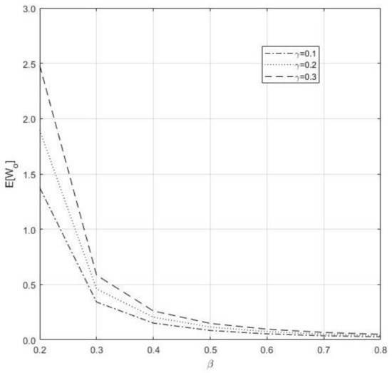 Figure 2. Impact of and on the .
 - (4)
- In Figure 3, if we increase both n and β, decreases.
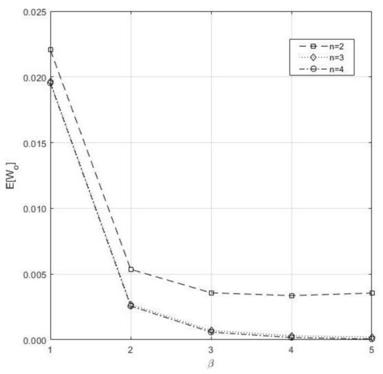 Figure 3. Impact of n and on the .
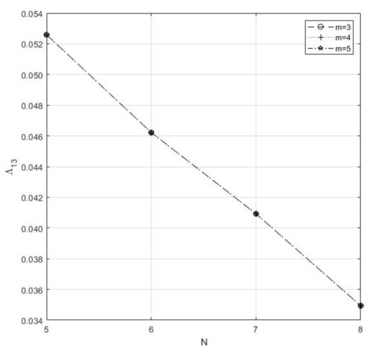
 - (5)
- From Figure 4, we conclude that γ cause an increase of when it is increasing, and n do the same as said in 4.
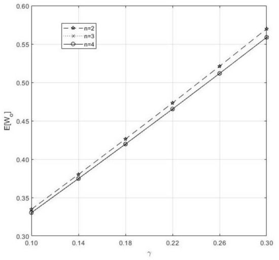 Figure 4. Impact of n and on the .
 - (6)
- Figure 5 explores the between and N. Here, we observe that and
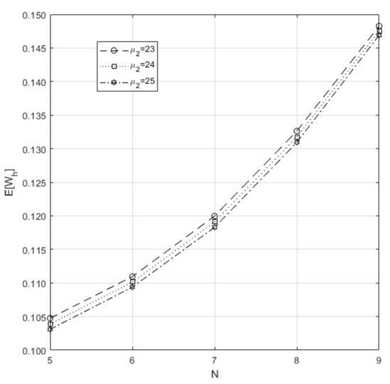 Figure 5. Impact of and N on the .
 - (7)
- In Figure 6, we realize that the parameter m and both react inversely to
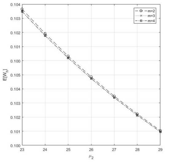 Figure 6. Impact of m and on the .
Example 3.
Here, we study the impact of customer loss of and streams. We can observe the following from Table 8 and Figure 7.
Table 8.
Customer lost for combination of n, m, , and q, r.
Figure 7.
Mean number of Type-II customer lost for m vs. N.
- (1)
- When we increase the number of servers, the lost for customer arrival become reduced. Since an increment in the ‘n’would reduce the number of busy servers, arrival can easily access the server.
- (2)
- When we increase q, the number of customer goes to orbit increases, i.e., customer loss is reduced.
- (3)
- The probability ‘r’ does the same role as q. That is, the increment in r sends the customer to the waiting hall after the service completion from . Here, we notice that variation in on r is considerably less than the on q.
- (4)
- The parameter γ causes the increment of deterioration of items which produce the customer lost; on the other hand, the impact of γ on would be less than .
- (5)
- As we increase the β, the existing stock level increases. It maintains the system having no insufficient stocks. Therefore, will decrease.
- (6)
- If we increase the waiting hall size N, this affects the decrement in the customer lost, as shown in Figure 7.
- (7)
- If we increase number of , the number of busy will decrease, and this affects the decrement in the customer lost, as shown in Figure 7.
Example 4.
In this example, we investigate the variation of the mean number of idle server for both and
- (1)
- When we increase the probability the mean number of idle server of becomes less, i.e., q decreases the arrival to the system when it is increasing, so it may happen that any number of becomes free. Suppose arrival() increases; there is a chance that all the server become busy as shown in Figure 8.
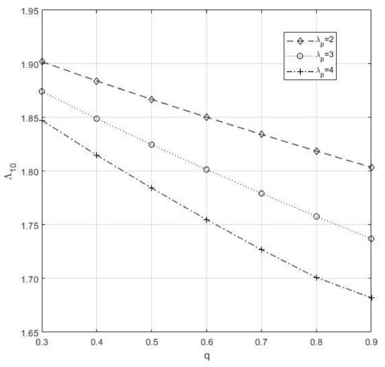 Figure 8. Mean number of Type-I Idle server of vs. q.
 - (2)
- If we do the increment in , service completion per unit time will increase so that this would impact the increase the , whereas does against μ, as shown in Figure 9.
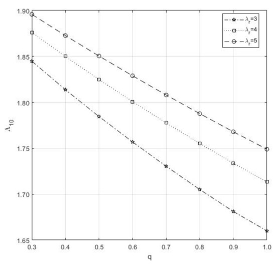 Figure 9. Mean number of Type-I Idle server of vs. q.
 - (3)
- From 1 and 2, and q preserve the said characteristic, as shown in Figure 10.
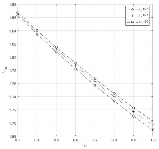 Figure 10. Mean number of Type-I Idle server of vs. q.
 - (4)
- If the parameter N and both cause the increment of , a mean number of busy server will increase, i.e., will decrease, as shown in Figure 11.
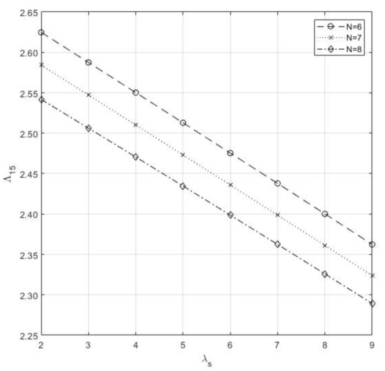 Figure 11. Mean number of Type-II Idle server of N vs. .
 - (5)
- The parameter N and both are reacting against each other, as shown Figure 12 on , i.e., N increases , whereas decreases
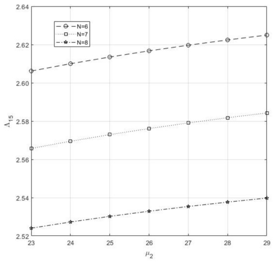 Figure 12. Mean number of Type-II Idle server of N vs. .
 - (6)
- In Figure 13, and preserve the said properties as in 4 and 5.
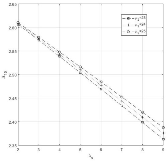 Figure 13. Mean number of Type-II Idle server of vs. .
6.2. Implication of the Proposed Model
In this model, we have a clear insight to fill many research gaps related to an interconnected optional arrival between two kinds of the dedicated identical multi-server service system in a queuing inventory sector. The ultimate aim of the model is to address the lack of discussion about an interconnected multi-server service system in a QIS. Accordingly, the considered MPQIS has the first major contribution: it admits the local convexity on its expected total cost in terms of optimum S and s under the variation of parameters and cost functions. Secondly, the waiting time of a T1 and T2 customer calculation has been carried out by varying the parameters. This work proves that the two multi-server service systems significantly reduce the waiting time of both T1 and T2. Further, the discussion of customer loss of both T1 and T2 and the number of idle servers of both T1S and T2S suggests how the findings are much needed to make an acceptable policy. Hence, we believe that our research findings of this MPQIS could constitute a critical source of intelligence because it has some risk of fixing the convexity, comparing the other (single multi-server) systems.
7. Conclusions
In the interconnected performance of two different multi-server service channels in the MPQIS, we discussed a Matrix geometric technique for two types of arrival streams. The wait time distribution for both streams is derived analytically by LST method. Subsequently, to fill the necessity of the proposed model in inventory management, we explored its functions numerically in all examples. In nature, the environment is relatively unstable. Firms are ready to make a significant change by creating opportunities for their demands. All the firms must study the factors that are very useful to redefine their value potentially at regular intervals, and this can assist and generate a new strategy to manage the emerging problems around the industry when approaching a generic model in stochastic queuing modeling, as well as would deliver a well-build and predicted results successfully. Moreover, this technique provides a positive variance which can expose a business, as to whether it is on the right track. In such a way that, the approached model would benefit the inventory industrialists and managements. The proposed model can also be an applicable on computational intelligence consisting electronic-based sensor technologies in the field of smart inventory management. In the future, we are planning to develop this model in a Markovian arrival process with the Phase-type distribution environment.
Author Contributions
Conceptualization, K.J. and N.A.; Data curation, K.J. and S.S.; Formal analysis, K.J. and T.H.; Funding acquisition, R.D. and G.P.J.; Investigation, S.A. (S. Amutha) and S.A. (Srijana Acharya); Methodology, T.H., S.A. (S. Amutha) and S.A. (Srijana Acharya); Project administration, R.D. and G.P.J.; Software, T.H.; Supervision, G.P.J.; Validation, S.S. and S.A. (Srijana Acharya); Visualization, S.A. (S. Amutha); Writing—original draft, N.A.; Writing—review & editing, G.P.J. All authors have read and agreed to the published version of the manuscript.
Funding
Anbazhagan and Amutha would like to thank RUSA Phase 2.0(F 24-51/2014-U), DST-FIST(SR/FIST/MS-I/2018/17), DST-PURSE 2nd Phase programme (SR/PURSE Phase 2/38) and UGC-SAP(DRS-I)(F.510/8/DRS-I/2016(SAP-I)), Govt. of India.
Data Availability Statement
The data presented in this study are available on request from the corresponding authors.
Conflicts of Interest
The authors declare no conflict of interest.
Notations
| 0 | zero matrix |
| e | A column vector of covenient size having one in each co-ordinates |
| em(n) | A column vector of dimension m with 1 in the n-th position |
| In | An identity matrix of order n |
| W | Whole numbers |
| M | Cut-off point of the truncation process in the matrix geometric approximation |
| entry at (a, b)th position of a matrix | |
| Kronecker product of matrices Z1 and Z2 | |
| X1(t) | Number of customers in the orbit at time |
| X2(t) | Number of items in the inventory at time t |
| X3(t) | Number of busy T1S at time t |
| X4(t) | Number of T2 customers (waiting and being served) in the waiting hall at time t |
| X5(t) | Number of busy T2S at time t |
| S | Maximum inventory level |
| s | Reorder point |
| S* | Optimum inventory level |
| s* | Optimum reorder point |
| Intensity rate of T1 arrival | |
| Intensity rate of T2 arrival | |
| Intensity rate of retrial arrival | |
| Intensity rate of T1 service | |
| Intensity of T1 arrival | |
| β | Intensity rate of reordering item |
| γ | Intensity rate of deteriorating item |
| ch | Inventory carrying costs per unit time |
| cs | Setup cost per unit time |
| cp | Perishable cost per unit time |
| T1 customers’ waiting cost per unit time | |
| T1 customers’ lost cost per unit time | |
| T2 customers’ lost cost per unit time | |
| T2 customers’ waiting cost per unit time | |
| TC | Total expected cost |
| TC* | optimum expected total cost |
| N | Size of the waiting hall |
| Vk | {1, 2, …, k} |
| E1 | |
| E2 | |
| E3 | |
| E4 | |
| D | |
| C | |
References
- Melikov, A.Z.; Molchanov, A.A. Stock Optimization in Transport/Storage. Cybern. Syst. Anal. 1992, 28, 484–487. [Google Scholar] [CrossRef]
- Sigman, K.; Simchi-Levi, D. Light traffic heuristic for an M/G/1 queue with limited inventory. Ann. Oper. Res. 1992, 40, 371–380. [Google Scholar] [CrossRef]
- Berman, O.; Kaplan, E.H.; Shimshak, D.G. Deterministic Approximations for Inventory Management at Service Facilities. IIE Trans. 1993, 25, 98–104. [Google Scholar] [CrossRef]
- Berman, O.; Kim, E. Stochastic Inventory Policies for Inventory Management at Service Facilities. Stoch. Models 1999, 15, 695–718. [Google Scholar] [CrossRef]
- Berman, O.; Sapna, K.P. Inventory Management at Service Facilities for Systems with Arbitrarily Distributed Service Times. Stoch. Models 2000, 16, 343–360. [Google Scholar] [CrossRef]
- Manual, P.; Sivakumar, B.; Arivarignan, G. A Perishable inventory system with service facilities and retrial customers. Comput. Ind. Eng. 2008, 54, 484–501. [Google Scholar] [CrossRef]
- Amirthakodi, M.; Sivakumar, B. An inventory system with service facility and finite orbit size for feedback customers. OPSEARCH 2014, 52, 225–255. [Google Scholar] [CrossRef]
- Amirthakodi, M.; Radhamani, V.; Sivakumar, B. A perishable inventory system with service facility and feedback customers. Ann. Oper. Res. 2015, 233, 25–55. [Google Scholar] [CrossRef]
- Jeganathan, K.; Anbazhagan, N.; Kathiresan, J. A Retrial Inventory System with Non-Preemptive Priority Service. Int. J. Inf. Manag. Sci. 2013, 24, 57–77. [Google Scholar]
- Jeganathan, K.; Kathiresan, J.; Anbazhagan, N. A retrial inventory system with priority customers and second optional service. OPSEARCH 2016, 53, 808–834. [Google Scholar] [CrossRef]
- Melikov, A.Z.; Shahmaliyev, M.O. Queueing System M/M/1/∞ with Perishable Inventory and Repeated Customers. Autom. Remote Control. 2019, 80, 53–65. [Google Scholar] [CrossRef]
- Reshmi, P.S.; Jose, K.P. A MAP/PH/1 Perishable Inventory System with Dependent Retrial Loss. Int. J. Appl. Comput. Math. 2020, 6, 1–11. [Google Scholar] [CrossRef]
- Kuo-Hsiung, W.; Keng-Yuan, T. A queueing system with queue dependent servers and finite capacity. Appl. Math. Model. 2000, 24, 807–814. [Google Scholar]
- Bae, J.; Kim, J.; Lees, E.Y. An optimal service rate in a Poisson arrival with two-stage queue service policy. Math. Methods Oper. Res. 2003, 58, 477–482. [Google Scholar] [CrossRef]
- Jeganathan, K.; Reiyas, M.A.; Padmasekaran, S.; Lakshmanan, K. An M/EK/1/N Queueing-Inventory System with Two Service Rates Based on Queue Lengths. Int. J. Appl. Comput. Math. 2017, 3, 357–386. [Google Scholar] [CrossRef]
- Jeganathan, K.; Reiyas, M.A.; Prasanna Lakshmi, K.; Saravanan, S. Two server Markovian inventory systems with server interruptions: Heterogeneous vs. homogeneous servers. Math. Comput. Simul. 2019, 155, 177–200. [Google Scholar] [CrossRef]
- Jeganathan, K.; Sumathi, J.; Mahalakshmi, G. Markovian Inventory Model With Two Parallel Queues, Jockeying And Impatient Customers. Yugosl. J. Oper. Res. 2016, 26, 467–506. [Google Scholar] [CrossRef]
- Pandelis, D.G. Optimal stochastic scheduling of two interconnected queues with varying service rates. Oper. Res. Lett. 2008, 36, 492–495. [Google Scholar] [CrossRef]
- Jeganathan, K.; Melikov, A.Z.; Padmasekaran, S.; Jehoashan Kingsly, S.; Prasanna Lakshmi, K. A Stochastic Inventory Model with Two Queues and a Flexible Server. Int. J. Appl. Comput. Math. 2019, 5, 1–27. [Google Scholar] [CrossRef]
- Jeganathan, K.; Reiyas, M.A. Two parallel heterogeneous servers Markovian inventory system with modified and delayed working vacations. Math. Comput. Simul. 2020, 172, 273–304. [Google Scholar] [CrossRef]
- Krishnamoorthy, A.; Manikandan, R.; Shajin, D. Analysis of a Multiserver Queueing-Inventory System. Adv. Oper. Res. 2015, 2015, 1–16. [Google Scholar] [CrossRef]
- Rajkumar, M.; Sivakumar, B.; Arivarignan, G. An infinite waiting hall at a multi-server inventory system. Int. J. Inventory Res. 2014, 2, 189–221. [Google Scholar] [CrossRef]
- Arivarignan, G.; Yadavalli, V.S.S.; Sivakumar, B. A perishable inventory system with multi-server service facility and retrial customers. Manag. Sci. Pract. 2008, 3–27. [Google Scholar]
- Yadavalli, V.S.S.; Sivakumar, B.; Arivarignan, G.; Olufemi, A. A Multi-Server Perishable Inventory System With negative customer. Comput. Ind. Eng. 2011, 61, 254–273. [Google Scholar] [CrossRef]
- Nair, A.N.; Jacob, M.J.; Krishnamoorthy, A. The multi server M/M/(s,S) queueing inventory system. Ann. Oper. Res. 2013, 233, 321–333. [Google Scholar] [CrossRef]
- Wang, F.; Bhagat, A.; Chang, T. Analysis of priority multi-server retrial queueing inventory systems with MAP arrivals and exponential services. OPSEARCH 2017, 54, 44–66. [Google Scholar] [CrossRef]
- Paul, M.; Sivakumar, B.; Arivarignan, G. A Multi-Server Perishable Inventory System With Service Facility. Pac. J. Appl. Math. 2009, 2, 69–82. [Google Scholar]
- Suganya, C.; Sivakumar, B.; Arivarignan, G. Numerical investigation on MAP/PH(1), PH(2)/2 inventory system with multiple server vacations. Int. J. Oper. Res. 2017, 29, 1–32. [Google Scholar] [CrossRef]
- Suganya, C.; Sivakumar, B. MAP/PH(1), PH(2)/2 finite retrial inventory system with service facility, multiple vacations for servers. Int. J. Math. Oper. Res. 2019, 15, 265–295. [Google Scholar] [CrossRef]
- Yadavalli, V.S.S.; Sivakumar, B.; Arivarignan, G.; Olufemi, A. A finite source multi-server inventory system with service facility. Comput. Ind. Eng. 2012, 63, 739–753. [Google Scholar] [CrossRef]
- Gabi, H.; Tal, A.; Tatyana, C.; Uri, Y. A multi-server system with inventory of preliminary services and stock-dependent demand. Int. J. Prod. Res. 2020, 1–19. [Google Scholar]
- Cheng-Yuan, K.; Scott, J. Access Control to Two Multiserver Loss Queues in Series. IEEE Trans. Autom. Control. 1997, 42, 1017–1023. [Google Scholar] [CrossRef][Green Version]
- Neuts, M.F. Matrix-Geometric Solutions in Stochastic Models—An Algorithmic Approach; Dover Publication Inc.: New York, NY, USA, 1981. [Google Scholar]
- Abate, J.; Ehitt, W. Numerical inversion of laplace transformation of probability distributions. ORSA J. Comput. 1995, 7, 36–43. [Google Scholar] [CrossRef]


Publisher’s Note: MDPI stays neutral with regard to jurisdictional claims in published maps and institutional affiliations. |
© 2021 by the authors. Licensee MDPI, Basel, Switzerland. This article is an open access article distributed under the terms and conditions of the Creative Commons Attribution (CC BY) license (http://creativecommons.org/licenses/by/4.0/).