1. Introduction
Fractional order differential equations have found an important role in the analysis and modelling of various processes. The fundamentals of fractional calculus and its most interesting application areas can be found in [
1,
2,
3,
4,
5,
6,
7]. In recent years, fractional calculus has appeared to be a modern and prospective tool for modelling and analysis of different processes of dynamic behaviour.
In control theory, one of the most useful methods of analysis and synthesis of control systems is to express the problem under consideration in the state-space equations form. The differential equations are transformed to a set of equations that can be written in the form of a differential matrix equation. If the process has a fractional nature, we obtain the state-space equations of a fractional order system. The most popular class of fractional order systems has a common order of fractional derivative for all components of a state vector. These systems are widely considered in the literature [
1,
5,
8,
9]. The case where the orders of each component of the state vector are different is not that popular or developed by researchers. The different order fractional systems were investigated in [
1,
10,
11] and applied to the analysis of transient states in electrical circuits in [
5,
12,
13,
14]. In the aforementioned papers, only Caputo or Riemann–Liouville definitions of fractional order derivatives were used. In the literature, solutions of the state equations with different orders of differentiation can be found in the case of the definition of the derivative expressed by the Caputo definition in [
1]. Theoretical analysis has not been verified in the experimental way.
The problem of time-domain analysis of a single fractional-order element has been considered in [
15], where analytical considerations for fractional order inductors and fractional order capacitors based on Caputo definition and numerical simulations were presented. Similar considerations were conducted for an electrical circuit consisting of two fractional order electrical elements in [
16]. Additionally, the problem of oscillations in such systems based on the Routh table method was investigated.
Recently, many new definitions of fractional order or so-called pseudo-fractional order derivatives have appeared. Khalil et al. introduced in [
17] a new operator of noninteger order called Conformable Fractional Derivative (CFD). In [
18], it was shown that the properties of this new derivative are very similar to integer order (classical) derivatives. Moreover, this new operator is numerically efficient in comparison with the older fractional order derivatives of Caputo or Riemann–Liouville. The CFD fractional differentiation was applied for the analysis of electrical circuits in state space in [
19,
20,
21].
In this paper, the authors apply the theory of different order fractional continuous-time systems to the theoretical and experimental analysis of an electrical circuit with two fractional order elements of different orders. The fractional order element can be realized in the form of a ladder circuit consisting of passive elements R,
L, C. In theory, a ladder system can behave as a fractional-order element only if it has an infinite number of components (infinite number of meshes). In practice, this number is always finite, which results in limitations related to the range of applications in which we could regard a ladder system as an element of fractional order. For this reason, it is important to properly select the resistance and capacitance—so that for a given number of elements we obtain a circuit that behaves with the highest possible accuracy and in the broadest possible frequency range as an element of fractional order [
22,
23,
24,
25,
26].
During the analysis of the fractional order electrical circuit, we formed the state-space model and analysed this system taking into account different types of derivative operators: Caputo, conformable fractional derivative and classical first-order derivative. The results of the numerical analysis are compared with the measurements of the voltages in the circuit. It is shown that the accuracy of the model differs significantly if we change the operator of derivation. The best modelling quality is achieved for the Caputo type model. It is shown that the classical approach of the model with a standard integer-order derivative does not allow one to obtain the precise description of the dynamic behaviour of the considered process.
The paper has the following structure. In
Section 2, the fractional order derivative definitions of Caputo and CFD are presented. Next, in
Section 3, the different fractional order state-space model is introduced and the general solution formulas of the model are given for the classical case of the integer-order derivative and the aforementioned fractional derivatives.
Section 4 is devoted to the processes of designing and construction of electrical elements composed of resistors and capacitors, which are used in
Section 5 to build a two fractional-order electrical circuit. Next, the theoretical considerations of the state-space model of the circuit are verified by laboratory measurements. Conclusions that follow from the theoretical and experimental analysis are in
Section 6.
3. Fractional Order State-Space Equations
Consider a fractional linear system described by the equation [
1]
where
are the appropriate fractional order derivative operators:
for the Caputo type derivative (
1),
for CFD Definition (
2), and first-order derivative operator
in the classic case. In our considerations, we will assume that the orders of derivatives are
and
. The state variables
and
and the input
are scalar functions of time,
and
are constant real coefficients, where
. Initial conditions are defined by
.
The solution of the state Equation (
4) can be written in the following form [
1]
where the functions
,
,
have different forms depending on the considered derivative definition.
In the case where we use a Caputo definition of fractional order derivative in (
4), the functions take the form
where the matrices
are given in the following recursive form
and
is the
identity matrix and
In the case of CFD definition, the functions
,
,
take the form [
21]
where matrices
and
are defined by Formula (
8).
The classical case is obtained by substituting in Formula (
9)
. Then we have
where
Now, let us consider state Equation (
4) with zero initial conditions
, a constant control
, and a nonsingular matrix
A.
In the considered case, the solution that describes the step response of the system is given by the formula
In this section, the fractional different order state-space equations were presented. The solutions to the model were considered for three cases of derivative operators: Classical integer-order derivative, Caputo, and CFD fractional derivatives.
4. Design and Construction of Fractional Elements
To validate the results shown in the previous section, we designed and constructed an electrical circuit consisting of two RC ladder elements which may be modelled with fractional order derivatives. Each element has a different order.
There are many papers where the practical realization problem of a fractional order element (device) has been described [
22,
23,
24,
28,
29,
30]. A fractional device is implemented as a tree, chain or net grid type connection of resistances, inductors and capacitors with appropriate values for its rated parameters.
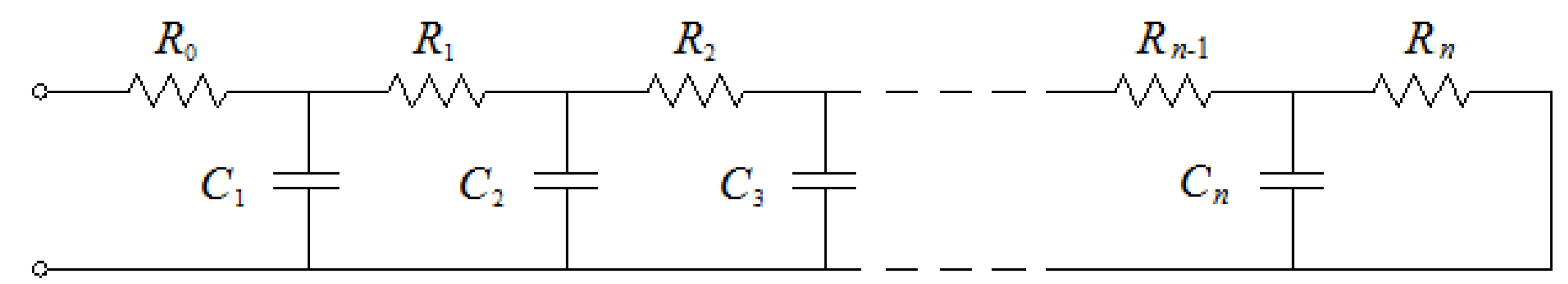
In this paper, we focus on the Cauer I type network shown in
Figure 1. This ladder structure requires proper selection of passive components R and C [
22,
23,
24] in order to obtain the desired order.
In many articles, different methods of fractional-order ladder realization are considered and compared. Most of them assume that the order of the fractional power of
s is 0.5 or a multiple of this value. The comparison of different approaches is given in [
31].
In our research, we are interested in the electrical circuit with at least two different order fractional elements of the values from the interval . The second important issue is to choose the frequency interval in which the phase characteristic of a ladder element is constant. In our case, we assume that the designed elements will have a constant phase angle for frequencies from 1 Hz to 10 kHz.
In the choice of a Cauer I type structure of the RC ladder, we took into account the simplicity of physical implementation and the availability of the electrical elements of the parameters required by the project. Moreover, in this complex optimization problem of parameter (values of resistances and capacitances) choice, the Cauer I type structure appears as the most numerically efficient.
The impedance of the ladder circuit shown in
Figure 1 is given by the formula [
22,
23,
24]
where
and
for
are the resistances and capacitances of the circuit.
The fraction of the chain (
13) may be expressed in the equivalent form of the following rational transfer function
where
and
are the
n-th degree polynomials and
n is the length of the practical realization.
The perfect element (infinite ladder) of fractional order
with pseudocapacity
has an impedance
Therefore, the proper design process of ladder circuits with fractional order properties requires an approximation of the power function
by the rational Function (
14), i.e., we should choose the values of resistances and capacitances such that
for the desired range of frequency.
One of the approximation methods is based on the development of the expression
with the Continuous Fractional Expansion (CFE) method [
28,
29,
30].
Due to the finite degrees of polynomials appearing in the numerator and denominator of (
14), the continued fraction should be terminated at a certain moment, allowing for an approximation of the
n-th order of the expression
We substitute into Formula (
17)
, and then we reduce the resulting continued fraction to the form of a rational function
where
is called the central angular frequency, and the corresponding coefficients are given by the following relations [
28,
29,
32]
where
is the Newton binomial coefficient, and
is the Pochhammer symbol.
We apply approximation (
18) in Formula (
15) and we get
We take the right side of the Equation (
22) as the rational function, being the approximation of the impedance (
14)
Knowing the form (
23) of the impedance of the ladder circuit shown in
Figure 1, we may calculate the value of resistances and capacitors required for its proper implementation.
The described CFE method allows the design of two ladder systems that have different orders concerning the differential operator. The parameters of these elements are presented in
Table 1.
In this section, we briefly describe the synthesis process of the fractional order elements with desired parameters. Two electrical ladders were designed with fractional orders and , which are used in the analysis of the different order fractional electrical circuit. The ladders have a constant phase angle in the desired frequency interval from 1 Hz to 10 kHz with a relative error less than .
5. Fractional Order Electrical Circuit
Consider an electrical circuit that consists of five resistors and two RC ladder elements of different fractional orders described in the previous section and denoted by triangles in the diagram shown
Figure 2. The input voltage is a step signal with magnitude
. The initial voltages across the capacitors are assumed to be zero, i.e.,
and
.
We will measure the voltages across the fractional order elements, i.e., the outputs of our system will be voltages and .
The current in the element of the fractional order is expressed by the formula
where
are pseudo-capacities (capacity in the classical case,
in the case of CFDs, and
in the Caputo definition case), while
are the appropriate fractional operators—the first derivative operator in the classical case, the operator
defined in the case of CFD definition and operator
in the Caputo definition case.
Based on the diagram shown in
Figure 2, we may write the state-space equation for the electrical circuit
where
and the elements of the matrix are as follows
while the components of the vector are given by
where
Note that the matrix
A is a nonsingular matrix, since
Therefore, the solution of the Equation (
25) will be similar to the solution (
12)
where
is a vector independent of pseudocapacity, i.e., also of the applied definition of a fractional order derivative.
Depending on the considered fractional definition, the function
will have a different form. In the case of the Caputo definition, we obtain a functional series on the basis of (
6)
except that instead of a matrix
we use matrices
, which are related by a relationship
, which leads to the following recursive relationship
where
If we choose a CFD derivative definition, the function
may be calculated using Formulas (
9), (
26), and (
35)
We treat the classical case as a special variant of Formula (
36), for
and
, i.e.,
Table 2 shows the values of resistances of the resistors
in the circuit shown in
Figure 2.
Based on the data from
Table 2 and Formula (
27) and matrices (
35) we calculated the matrices
The circuit was supplied by the step voltage with magnitude V.
Substituting the values of the resistance into Equation (
32) we may compute a voltage vector in a steady state
The electrical circuit was based on the diagram shown in
Figure 2 and was supplied with a step voltage signal from a functional generator NI PXI–5402. The experimental data for the performed ladder systems were obtained during measurement of time-voltage characteristics and have the form of a set
, where
are the voltages measured across the fractional order ladder systems at time instants
, wherein
ms is the sampling period, while the number of measurements was selected experimentally in such way that
.
For the circuit under consideration, we know the general form of the solution of state equation (
31) and we take into account steady-state voltage vector (
39) as well as matrices
and
in (
38). We may also assign an appropriate function
for the Caputo definition case (
33), for CFD derivative (
36) and for the classical first-order derivative case (
37).
We shall find the parameters of the fractional order elements depending on the differential operator used in each model (orders of the derivative, values of pseudo-capacity or capacity). In the case of the Caputo model, we may take the values from
Table 1. For the remaining cases of the models with CFD and classical derivatives, the appropriate parameters should be estimated. To find an optimal value of the parameters, we use a series of measurement data with the cost function of the form
where
are the values taken from the state equation models.
A set of acceptable values of the parameter vector varies depending on the model that is currently considered. In the classical case of the first-order derivative, we have , while in the case of CFD definition we have a set:
.
5.1. CFD Model
The estimated values for the CFD model are presented in
Table 3.
Substituting the estimated parameters of the fractional and pseudocapacitance from
Table 3 and matrices (
38) concerning Formula (
36), we obtain the form of the function used in solution (
31)
5.2. Classical Case Model
The values estimated in the classical case model are presented in
Table 4.
Substituting the estimated parameters from
Table 4 and matrix (
38) into Formula (
37), we obtain the form of the function used in solution (
31)
5.3. Caputo Model
Substituting the given parameters of the fractional order pseudocapacitance from
Table 1 into formula (
33), we obtain the form of the function used in solution (
31)
The matrix coefficients appearing in the function series (
43) have been defined by (
34) and the respective matrices and have the form (
38).
Figure 3 and
Figure 4 show the time characteristics of voltages across the fractional order ladder elements with
and
in an electrical circuit supplied by a step voltage signal
V. Additionally, based on solution (
31) and taking into account Functions (
41), (
42), and (
43) theoretical characteristics are simulated for each type of model.
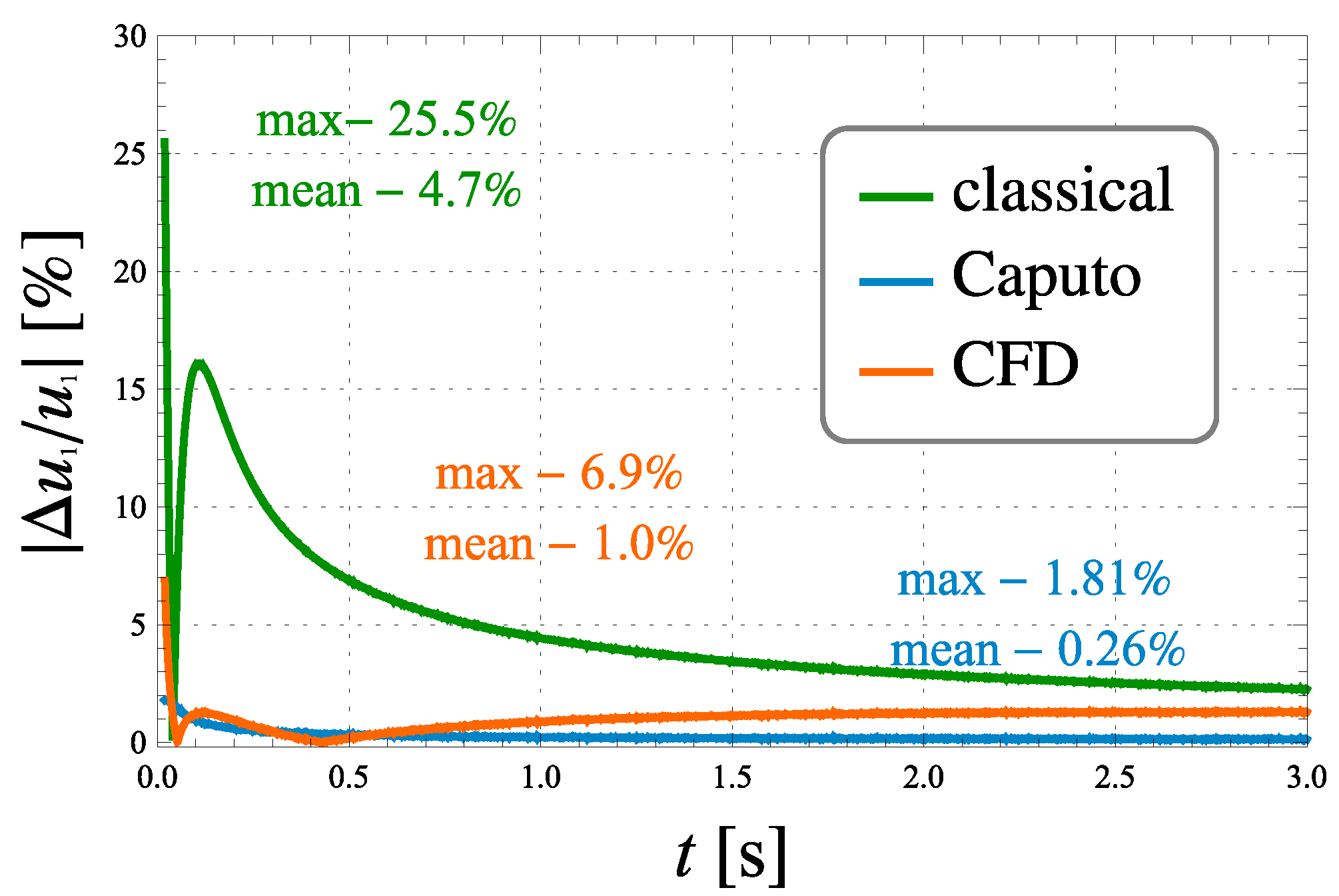
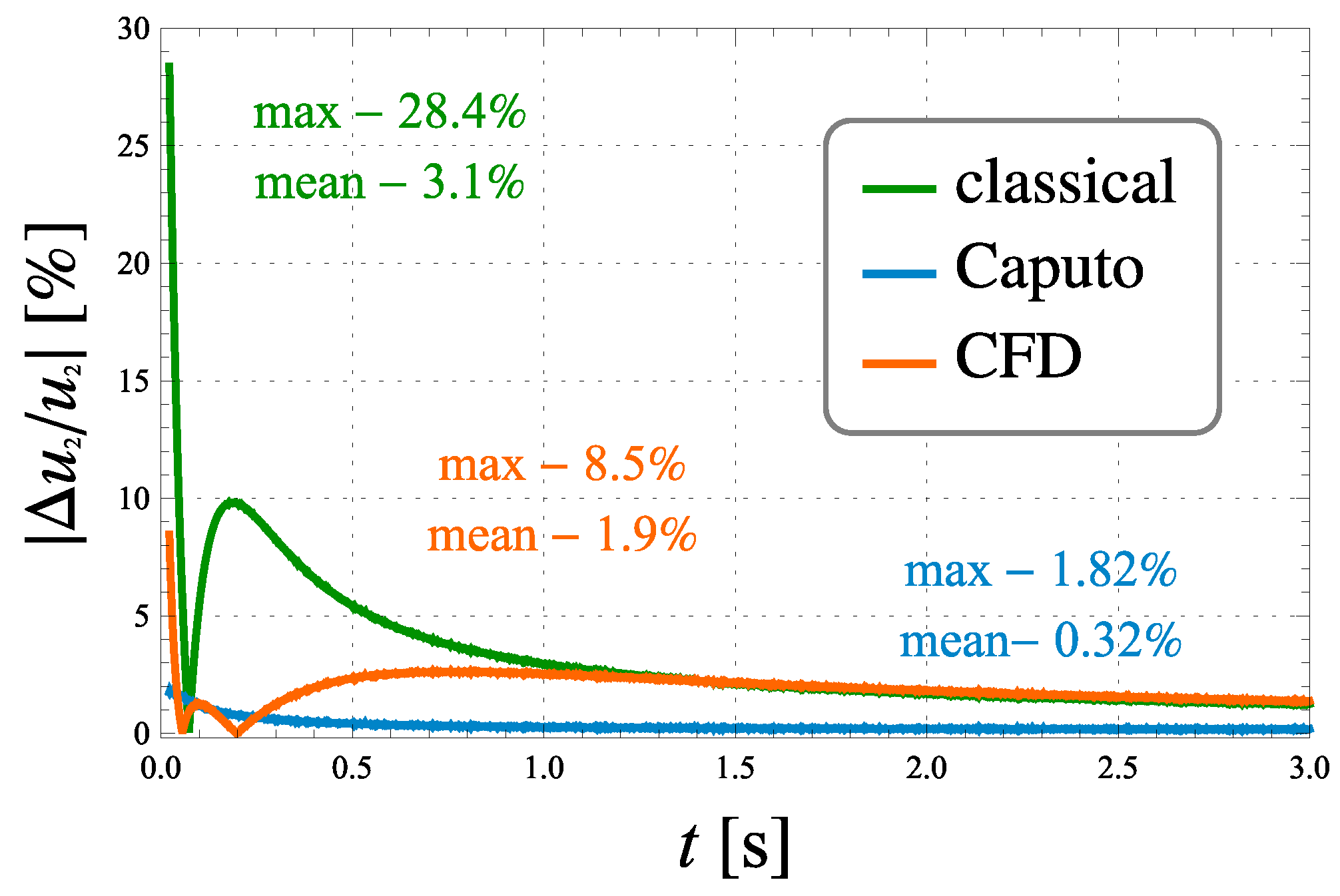
Comparing the real and theoretical time-voltage characteristics, we computed the relative errors, which are shown in
Figure 5 and
Figure 6.
Analysis of the characteristics shown in
Figure 3,
Figure 4,
Figure 5 and
Figure 6 implies that the model with classic integer-order derivative is highly inaccurate. This model is not able to reflect the dynamic behaviour of the process, especially the initial stage of charging, when the voltage changes across the fractional order ladder element are very rapid. The relative error of the time-voltage characteristics of the ladder systems reach a value exceeding 28.5%.
The model with the CFD derivative allows for greater precision of description, especially in the initial stage of loading. The maximum relative error is over three times smaller than in the classical case model and is no more than 8.5%. The time interval in which the response of the CFD model significantly differs from the experimental data is shorter than in the classical case model, which is reflected in the mean values of the relative errors.
The model based on the Caputo definition describes the dynamics of the voltage at the terminals of ladder circuits with the highest precision. The maximum relative error reaches 1.8%. The voltage characteristic of the Caputo model over longer periods of time is correct with a small value of the mean relative error, not more than 0.3%.


