Review

A Survey on Deep Learning Based Approaches for Scene Understanding in Autonomous Driving

School of Optical-Electrical and Computer Engineering, University of Shanghai for Science & Technology, Shanghai 200093, China
*
Authors to whom correspondence should be addressed.
These authors contributed equally to this work.
Electronics 2021, 10(4), 471; https://doi.org/10.3390/electronics10040471
Submission received: 21 December 2020 / Revised: 3 February 2021 / Accepted: 7 February 2021 / Published: 15 February 2021
(This article belongs to the Special Issue Autonomous Vehicles Technology)

Abstract

:
As a prerequisite for autonomous driving, scene understanding has attracted extensive research. With the rise of the convolutional neural network (CNN)-based deep learning technique, research on scene understanding has achieved significant progress. This paper aims to provide a comprehensive survey of deep learning-based approaches for scene understanding in autonomous driving. We categorize these works into four work streams, including object detection, full scene semantic segmentation, instance segmentation, and lane line segmentation. We discuss and analyze these works according to their characteristics, advantages and disadvantages, and basic frameworks. We also summarize the benchmark datasets and evaluation criteria used in the research community and make a performance comparison of some of the latest works. Lastly, we summarize the review work and provide a discussion on the future challenges of the research domain.

1. Introduction

Scene understanding, positioning and navigation, path planning, and control execution are the four basic modules in an autonomous driving system, among which scene understanding is the core module. As described in [1], the complex task of outdoor scene understanding involves several subtasks such as object detection, scene categorization, depth estimation, tracking, event categorization and behavior analysis. Sense understanding acts as human eyes do, and it is a prerequisite for autonomous driving.
In the past ten years, machine learning using convolutional neural networks (CNNs) has moved from shallow machine learning to deep machine learning with the advancement of neural network theory and the improvement of hardware computing capabilities. The shallow machine learning model does not use distributed representation and requires artificially extracted features. The quality of the artificially extracted features largely determines the quality of the entire system. Deep learning is a kind of representation learning that can learn higher-level abstract representations of data and automatically extract features from the data. The hidden layers in deep learning are equivalent to a linear combination of input features, and the weights between the hidden layers and the input layer are equivalent to the weights of the input features in the linear combination. The learning capability of deep learning increases exponentially with the depth of the model. CNN is the most common deep learning methodology applied to autonomous driving. A CNN is parametrized by its weights vector θ = [W, b], where W is the set of weights governing the interneural connections and b is the set of neuron bias values. The set of weights W can be learned from the data during the training process. The convolutional layers within a CNN exploit the local spatial correlations of image pixels to capture image features. The last layer of a CNN is usually a fully connected layer, which acts as an object discriminator for a high-level abstract representation of objects. CNN-based deep learning can learn higher-level abstract representations of data and automatically extract features. Due to these advantages, CNN-based deep learning approaches have been widely used in scene understanding of autonomous driving, and it has achieved great success. This paper presents a survey on research using deep learning-based approaches for scene understanding in autonomous driving, especially focusing on two main tasks: object detection and scene segmentation. Similar surveys have been found in [2,3], with [2] specifically providing an overview on deep learning-based applications covering almost all aspects of autonomous driving, including perception and localization, high-level path planning, behavior arbitration, and motion controllers. Our paper only focuses on one specific area: scene understanding. Comparatively, our paper provides much more detail of the algorithms for various scene understanding tasks. The deep-learning based approaches for scene text detection and recognition for the purpose of scene understanding were reviewed in [3]. Although it had the same goal as our paper, the algorithms were significantly different. To the best of our knowledge, our paper is the first comprehensive summary specifically focusing on vision-based deep-learning algorithms for scene understanding in automotive driving.
As illustrated in Figure 1, we categorized the research on scene understanding in autonomous driving into two streams: object detection and scene segmentation. Object detection is identifying and locating various obstacles in a road traffic scene in the form of bounding boxes, such as pedestrians, vehicles, and cyclists. Scene segmentation is assigning a semantic category label to each pixel in a scene image, and it can be regarded as a refinement of object detection. Scene segmentation can be further divided into three substreams: full-scene semantic segmentation, object instance segmentation, and lane line segmentation. A traffic scene normally contains object categories like obstacles, free space (roads), lane lines, and so on. Full-scene semantic segmentation is performing pixel-level semantic segmentation on these categories in a full image. Instance segmentation is designed to identify individual instances within a category area, and it can be regarded as a more elaborate semantic segmentation. As Neven et al. [4] mentioned, obstacles and free space are categories with relatively concentrated pixels, while lane lines are a pixel-continuous and non-dense category. It is difficult to segment lane lines and other objects at the same time in an image. Therefore, this paper surveys lane line segmentation as a special substream. As for the relations between the tasks, instance segmentation can not only provide pixel-level recognition but also distinguish individuals, which is more meaningful for autonomous driving but also a harder task. As a specific task, lane line recognition is indispensable for lane departure warnings and lane keeping applications. Figure 1 also illustrates the overall framework of this paper. The research on scene understanding is organized as four work streams, including object detection, full-scene semantic segmentation, instance segmentation, and lane line segmentation.
In terms of approaches, object detection is divided into two categories of methods: the two-stage method and the one-stage method. Full-scene semantic segmentation is divided into two categories of methods: encoder–decoder and modified convolution. As a special task in full-scene semantic segmentation, road segmentation is reviewed as a specific category. The approaches for instance segmentation are divided into region proposal and masking. Lane line segmentation is divided into the two-step method and the end-to-end method.
The remainder of the paper is structured as follows. In Section 2, the classification models (i.e., the basic deep CNN models) developed in the early years are reviewed, and the characteristics of the related algorithms are summarized. In Section 3, we discuss and analyze the research work of four work streams—object detection, full-scene semantic segmentation, instance segmentation, and lane line segmentation—according to their characteristics, advantages and disadvantages, and basic frameworks. Section 4 gives a performance comparison of some of the latest algorithms. Section 5 introduces the benchmark datasets and evaluation criteria accepted in the research society. Section 6 concludes with remarks and provides a discussion of the future challenges of the research domain.

2. Basic CNN Models

Deep learning-based object detection and scene segmentation actually originated from object classification; that is, classification models developed in the early years formed the basic models of detection and segmentation. Therefore, we give a brief overview of the object classification models in this section. The basic structure of deep CNNs can be traced back to LetNet, proposed by Lecun et al. [5] in 1990. It is composed of a convolutional layer, a pooling layer, a fully connected layer, and an activation function. In 2012, Krizhevsky et al. [6] extended LetNet to a deeper network—called AlexNet—capable of learning more complex features with the use of the ILSVRC database [7]. This work significantly improved the accuracy of image classification and initiated a continuous boom of deep learning research. Subsequently, VGGNet [8], GoogleNet [9], and ResNet [10] came along successively. Many lightweight deep neural networks came out one after another with continuous improvement of the network structure, such as ResNeXt [11], ShuffleNet [12], and so on. These excellent deep CNN models promoted the continuous breakthrough of computer vision tasks, such as object detection, semantic segmentation, and instance segmentation. Table 1 reviews the evolution of these CNNs in terms of the year, background, algorithm characteristics, and contributions.
These models are all suitable to be used as base models in autonomous driving to extract features for detection and classification purposes. In practice, the model should be selected via experiments according to applications. Generally, lightweight models are more suitable for tasks with larger datasets and can greatly reduce training time.

3. Scene Understanding in Autonomous Driving

In this section, we review deep learning-based approaches for scene understanding in terms of four work streams: object detection, full-scene semantic segmentation, instance segmentation, and line lane segmentation.

3.1. Object Detection

The approaches for object detection are divided into the two-stage method and the one-stage method. Table 2 gives a summary of the representative work in terms of their characteristics, advantages and disadvantages, and basic frameworks.

3.1.1. Two-Stage Method

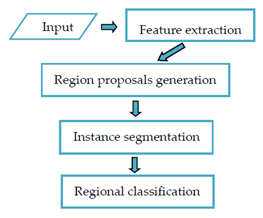
In 2014, Girshick et al. proposed an Region Based Convolutional Neural Networks (R-CNN) [20], which combines region proposal extraction and a CNN. It is the first algorithm that successfully applied deep learning to object detection, in which feature maps are extracted from a CNN rather than from the blockwise orientation histograms. The process of detection is shown in Figure 2. The method first generates a large number of regions using selective searching [35] and then extracts features on the region proposals using CNNs. However, the R-CNN has the following problems: (1) the extracted region proposals must be cropped or warped to a fixed size, resulting in missing information or a distorted image; (2) it is time-consuming, since it processed the region proposals separately; and (3) it is not an end-to-end network model.
He et al. proposed Spatial Pyramid Pooling Network (SPPNet) [21] in 2014 to address these issues. It still adopted region proposal, but proposed a pyramid pooling module to improve the efficiency of feature extraction of the R-CNN. It avoided the repeated calculation of region proposals and effectively solved the problems caused by cropping and warping. Girshic et al. [22] proposed Fast R-CNN to combine the advantages of both an R-CNN and SPPNet in 2015. It extracted features on the entire image and replaced the pyramid pooling module in SPPNet with the Region of Interest (ROI) pooling layers so that a fixed dimensional feature map was extracted for each region proposal. Furthermore, to address the problem of step-by-step training, it considered object detection as a border regression issue and proposed a multitask loss function for training. Since feature extraction was conducted on the entire image rather than processing the regions separately, it efficiently improved the computing efficiency. In addition, Fast R-CNN realized an end-to-end training process. Modifications within Fast R-CNN [22] indicate that region proposal is a bottleneck of computation. After that, Ren et al. [23] further improved Fast R-CNN to a newer version (i.e., Faster R-CNN) that replaced selective searching with a region proposal network (RPN) to obtain high-quality region proposals. Faster R-CNN is a fully convolutional network that simultaneously predicts object bounds and class scores at each position and can be trained end-to-end.
In this subsection, we introduced the development process of the two-stage method, starting from the R-CNN. It used selective searching to create a region proposal ingeniously. Although this affects computation efficiency, it provides a good idea for the object detection task. SPPNet, Fast R-CNN, and Faster R-CNN followed the idea. By designing the pyramid pooling module, ROI pooling, RPN, and other modules, they simplified region proposal generation and continuously improved the model training effectiveness. In summary, the two-stage method has good performance for object detection accuracy, but the detection speed is not high due to the complex structure. It is suitable for scenes with small objects.

3.1.2. One-Stage Method

In 2015, a one-step detection method called You Only Look Once-V1 (YOLO-V1) [24] was proposed by Redmon et al. It solved the detection speed issue, which has been troublesome in the two-stage detection methods [20,21,23]. The authors framed object detection as a regression problem to spatially separate the bounding boxes and associated class probabilities. A single neural network predicts bounding boxes and class probabilities directly from full images in one evaluation. Since the whole detection pipeline is a one-stage network, it can be optimized end-to-end directly for detection performance. The whole picture is predicted during both training and prediction, which effectively makes good use of the context information and therefore reduces the false detection rate.
In 2015, Liu et al. proposed Single Shot MultiBox Detector (SSD) [27] by combining the advantages of Faster R-CNN [23] and YOLO-V1 [26]. The network combines predictions from multiple feature maps with different resolutions to handle objects of various sizes. SSD eliminates proposal generations and subsequent pixels or feature resampling stages and encapsulates all computations in a single network. This makes SSD easy to train and straightforward to integrate into systems that require a detection component.
In 2017, Lin et al. [28] analyzed the problems between the accuracy and speed of the two-stage and the one-stage methods. They discovered that the extreme foreground–background class imbalance encountered during the training of dense detectors was the central cause. They proposed focal loss to address this class imbalance by reshaping the standard cross-entropy loss so that it downweighted the loss assigned to well-classified examples.
In 2017, Redmon et al. [29] improved YOLO-V1 to YOLO-V2 and YOLO9000, which can detect over 9000 categories. YOLO-V2 proposed a new basic network—Darknet-19—which greatly improved the detection performance, especially on small objects. The following year, YOLO-V3 [30], based on V1 [26] and V2 [29], was proposed. In terms of the network structure, it used ResNet [10] for reference and proposed a more complex backbone network (Darknet-53) to extract features. At the same time, Feature Pyramid Networks (FPN) [25] was added to improve the detection of multiscale objects. Compared with other models, it has obvious advantages in detection speed and further strengthens the detection ability for small objects.
In 2019, Tian et al. [31] proposed a fully convolutional one-stage object detector (FCOS) to solve object detection in a per pixel prediction fashion. FCOS is anchor box free, as well as proposal free. By eliminating the predefined set of anchor boxes, the FCOS completely avoids the complicated computations related to anchor boxes, such as calculating overlapping during training. More importantly, they also avoid all hyperparameters related to anchor boxes, which are often very sensitive to the detection performance. Chen et al. [33] used a RoIConv operator for alignment of the features and designed a fully convolutional architecture (AlignDet) for combining the flexibility of learned anchors and the preciseness of aligned features. Duan et al. [34] (CenterNet) modeled an object as a single point and used key point estimation to find the center point and then regressed to obtain object parameters, including size, location, and orientation. In 2020, GC-YOLOv3 [32] made YOLO-V3 more accurate with a global context block. They fused a feature extraction network with a feature pyramid network to improve detection accuracy.
Different from the two-stage method, this method does not have a separate stage for proposal generation. It typically considers all pixels as potential objects and tries to classify each region of interest as either the background or an object. In this subsection, we introduced the development process of the one-stage method starting from YOLO-V1. After that, YOLO V2–V4 followed. Later, a series of anchor-free object detectors (e.g., FCOS, AlignDet, and CenterNet) were developed, where the goal was to predict the key points of the bounding box instead of trying to fit an object to an anchor. In summary, the one-stage method reduced the difficulty of training and deployment. Compared with the two-stage method, the one-stage method is faster but with slightly poorer detection performance. They are more suitable for scenes with sparse populations, such as suburban villages.

3.2. Full-Scene Semantic Segmentation

Full-scene semantic segmentation is segmenting object categories at the pixel level in a full image. The approaches for full-scene segmentation are divided into two categories: encoder–decoder structure models and modified convolution structure models. As a specific and important task, road segmentation has been widely studied. Thus, we review road segmentation as the third subsection. Table 3 gives a summary of the representative works in terms of their characteristics, core technology and functions, basic frameworks, and road segmentation.

3.2.1. Encoder–Decoder Structure Models

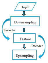
Different from object detection and classification, image semantic segmentation classification operates at the pixel level and thus is more difficult. The traditional semantic segmentation methods [55,56,57,58] rely on hand-crafted features that are usually tailored for a specific task. These methods do not offer ideal performance in terms of speed and accuracy. A breakthrough occurred in 2014, when Long et al. [36] proposed the fully convolutional network (FCN) and realized end-to-end pixel-level semantic segmentation. Its key insight is to build fully convolutional layers to automatically extract features for segmentation purposes. There are two main modifications: (1) The last fully connected layer of the CNN [8,9,10] is replaced by a convolution layer that outputs a size-reduced heatMap (segmented map). The structure of the network is actually an encoding process. (2) The segmented map is restored to the original size using bilinear interpolation. However, image restoring by this method lacks sensitivity to image details and will lead to rough and blurry segmentation. Moreover, the segmentation is based on the local area information without consideration of global information.
Badrnarayanan et al. [37] made an improvement on the FCN and proposed SegNet, which first adopted the encoder–decoder structure. SegNet consists of an encoder network and a corresponding decoder network, followed by a pixel-wise classification layer. The novelty of SegNet lies in the manner in which the decoder upsamples its lower resolution input feature maps. Specifically, the decoder uses pooling indices computed in the max pooling step of the corresponding encoder to perform non-linear upsampling. An illustration of the SegNet architecture is shown in Figure 3. This eliminates the need for learning to upsample. It does not involve deconvolution and greatly speeds up the training time. Many scene segmentation models adapt the encoder–decoder network structure, such as U-Net [38], ENet [39], RefineNet [59], and so on.
Semantic Segmentation Network (SegNet) ascertained the encoder–decoder structure and achieved significant progress in semantic segmentation. However, SegNet has a complex architecture and a large number of parameters, which makes the network run slower and not in real time. Paszke et al. [9] proposed ENet to improve computation efficiency in 2016. It learned from [14] to optimize the architecture through modular network design. The model adapted early downsampling, a large encoder, a small decoder, and nonlinear operation. Experiments showed that the model ran much faster than SegNet.
An FCN classifies objects at the pixel level, but it does not take context information into consideration. Thus, similarity between pixels may cause recognition confusion. In 2016, Zhao et al. [40] proposed the pyramid scene parsing network (PSPNet) to exploit the capability of global context information by different-region-based context aggregation. To reduce context information loss between different subregions, they used a hierarchical global prior, containing information with different scales. They called it the pyramid pooling module for global scene prior construction and put it upon the final layer feature map of the network. Recently, a novel pyramid self-attention module to overcome dilution problems in high-level semantic information was proposed in [60]. At the same time, a channel-wise attention module was also employed to reduce the redundant features of the FPN [25].
In this subsection, we introduced the development process of encoder–decoder models, starting from the FCN. SegNet, PSPNet, ENet, and U-Net followed the idea. By combining the PSP module, FPN, and attention module, the segmentation accuracy was continuously improved. Although these methods can achieve end-to-end pixel-level output, they are relatively slow and not ideal for segmenting small objects. They are more suitable for scenes with sparse populations such as suburban villages because they are based on local area information.

3.2.2. Modified Convolution Structure Models

In the basic CNN structure, the convolution layers are used to extract image features, and the pooling layers are used to gather image background information. However, the pooling layers cause problems, such as reducing the image resolution and losing local information. This leaves an open question of whether severe intermediate downsampling is truly necessary. Therefore, much research has been conducted to solve the above issues by modifying the convolution structure. A convolutional network module is needed that aggregates multiscale context information without losing resolution or analyzing resized images.
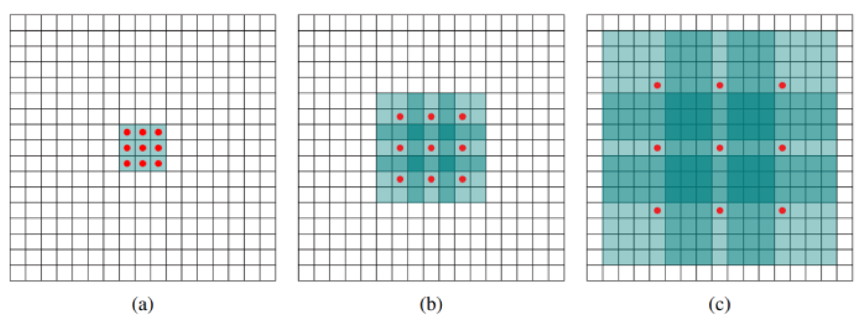
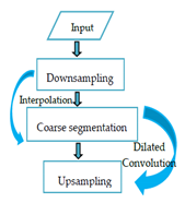
In 2014, Chen et al. [48] analyzed two problems of semantic segmentation models: (1) reducing the image size through pooled downsampling, resulting in information loss, and (2) the spatial invariance generated by the CNN. Then, they developed the DeepLab model. They skipped subsampling after the last two max pooling layers in the FCN and modified the convolutional filters by introducing zeros to increase their length. As shown in Figure 4, the modified convolution with zeros can increase the receptive field without changing the number of convolution kernels while the computation remains the same. The DeepLab model overcomes the poor localization properties of deep networks by using dilated convolution with a fully connected conditional random field (CRF) [61].
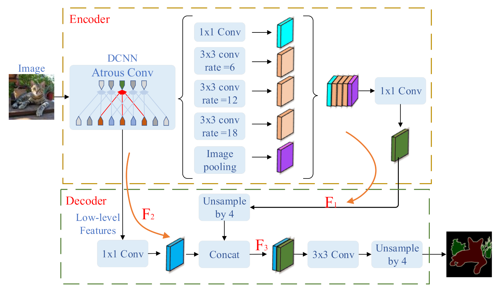
In 2017, Yu et al. proposed the Dilated Residual Network (DRN) [53] by combining dilated convolution with ResNet [10] and studying the gridding artifacts introduced by dilation. The gridding problem was solved by removing the maximum pooling layer, adding a network layer, and removing residual connections. Tests on the Cityscapes dataset [62] achieved good performance. In 2017, Chen et al. proposed DeepLab-V2 [50], based on DeepLab-V1 [48]. The most significant improvement was the combination of the dilated convolution structure and the pyramid network structure (21, 40). They proposed aerospatial pyramid pooling (ASPP) to segment objects with multiple scales. Atrous convolutions can also name dilated convolutions. To further handle the problem of segmenting objects at multiple scales, Chen et al. [51] proposed DeepLab-V3, which employed atrous convolution in cascade or in parallel to capture the multiscale context by adopting multiple atrous rates. The following year, Chen et al. pointed out that ASPP [50] could extract more dense features, but the existence of atrous convolution would cause the boundary information of the segmentation object to be seriously lost. It is known that the decoder structure can gradually recover spatial information to capture clear object boundaries. Accordingly, they proposed a model of the encoder–decoder structure with ASPP known as DeepLab-V3+ [41]. The network is composed of several representative structures, which makes it a leader in the field of semantic segmentation. The framework structure of DeepLab-V3+ is shown in Figure 5. Its processing visual results on Cityscapes [62] are shown in Figure 6.
In this section, we introduced region proposal-based methods and masking-based methods for instance segmentation. In general, the region proposal-based methods produce better accuracies than the masking-based methods. The challenges of instance segmentation still remain for small objects, as well as for efficient end-to-end models and their training schemes.

3.2.3. Road Segmentation

As an essential category in traffic scenes, the road is the area where a car can travel. Road recognition is of great significance for autonomous driving. Many researchers particularly focus on road segmentation. Up-conv-Poly [45] proposes an up-convolutional network for road segmentation by combining an FCN with U-Net [38]. The significant improvement was that it increased the width of the up-convolutional side of the network to improve the model accuracy. LidCamNet [46] fused lidar point clouds and camera images for road detection. The sparse point clouds are first projected onto the image plane and then upsampled to obtain a set of dense 2D images, encoding spatial information. Then, the FCN is trained to carry out road detection by using the fusing data. They designed three fusion strategies: early, late, and cross fusion. DEEP-DIG [47] used ResNet [10] with a fully convolutional architecture and multiple upscaling steps for image interpolation. On the basis of the FCN, it uses geometric transformations, such as affine and perspective transformation, image clipping, deformation, noise, and pixel changes, to obtain better road segmentation results. In addition, it attained encouraging improvement by performing data augmentation and conducting a number of training variants. Figure 7 shows the road segmentation results of Up-Conv-Poly, LidCamNet, and DEEP-DIG on the Karlsruhe Institute of Technology and Toyota Technological Institute (KITTI) dataset [63].

3.3. Instance Segmentation

Full-scene semantic segmentation only segments the categories within an image without consideration of object instances. Instance segmentation is designed to further segment individual object instances within a category area. From this point of view, instance segmentation is somewhat similar to object detection. Obviously, instance segmentation is useful for determining the motion state of individual obstacles, mainly referring to pedestrians and cars. The methods for instance segmentation can be divided into two classes: region proposal-based methods and masking-based methods. Table 4 gives a summary of the typical work in terms of their characteristics, advantages and disadvantages, and basic frameworks.

3.3.1. Region Proposal-Based Method

In 2014, Hariharan et al. [64] first proposed a network that was capable of detecting object instances and marking them at the pixel level. They called it simultaneous detection and segmentation (SDS). Unlike classical bounding box detection, SDS requires pixel-level segmentation for individual instances. The technical process is shown in Figure 8. The following year, they defined the hypercolumn [65] at a pixel as the vector of activations of all CNN units above that pixel. The main idea is to use the columns as pixel descriptors, which combine the low-level features with the high-level features to improve the optimization of details.
SDS [64] and hypercolumns [65] are too time-consuming to select a large number of region proposals. Moreover, they do not make the best use of the learned deep features and large-scale training data. In 2015, Dai et al. presented multitask network cascades (MNC) [66] for instance-aware semantic segmentation. Their model consisted of three networks, respectively differentiating instances, estimating masks, and categorizing objects. These networks form a cascaded structure and are designed to share their convolutional features. An Instance-Sensitive Fully Convolutional Network (ISFCN) [67] further enhanced the method and learned from the position-sensitive score map in the R-FCN [24] to improve the local pixel segmentation. Such a cascading framework is also used in the Fully Convolutional Instance-Aware Semantic Segmentation (FCIS) [68].
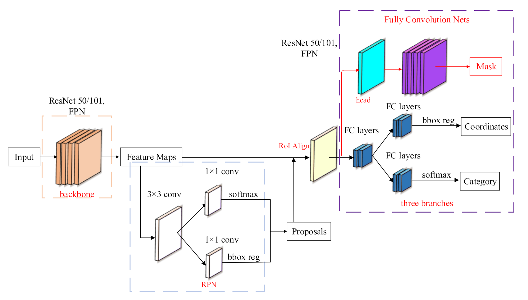
In 2017, He et al. [69] extended Faster R-CNN by adding a branch for predicting an object mask in parallel with the existing branch for bounding box recognition. The region of interest is generated for the first time, and then these ROIs are classified and subdivided in the second stage. An illustration of the Mask R-CNN architecture is shown in Figure 9.
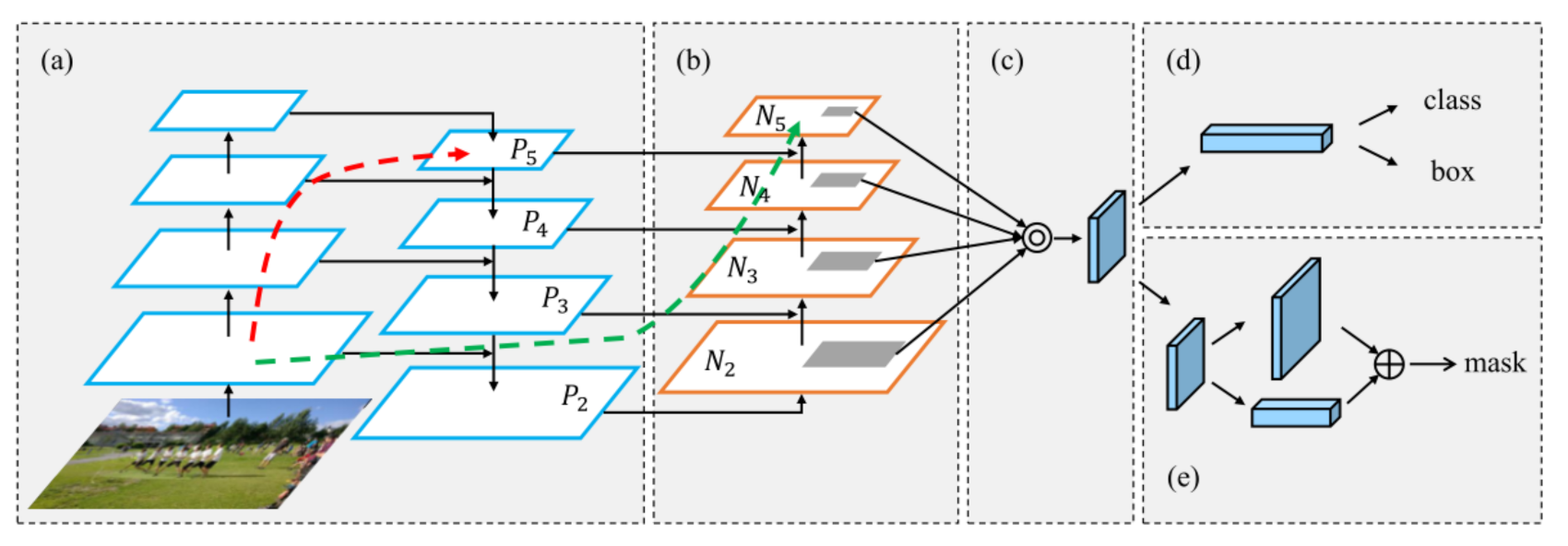
In 2018, Liu et al. [70] proposed the path aggregation network (PANet), aimed at boosting information flow in a proposal-based instance segmentation framework. Specifically, they enhanced the entire feature hierarchy with accurate localization signals in the lower layers by bottom-up path augmentation, which shortened the information path between the lower layers and the topmost feature. As shown in Figure 10, three main improvements were made: (1) improving the FPN by using bottom-up path augmentation; (2) improving the pooling strategy by using adaptive feature pooling; and (3) improving the mask branch by using fully connected fusion. The visualization results of the Path Aggregation Network (PAN) can be shown in Figure 11.

3.3.2. Masking-Based Method

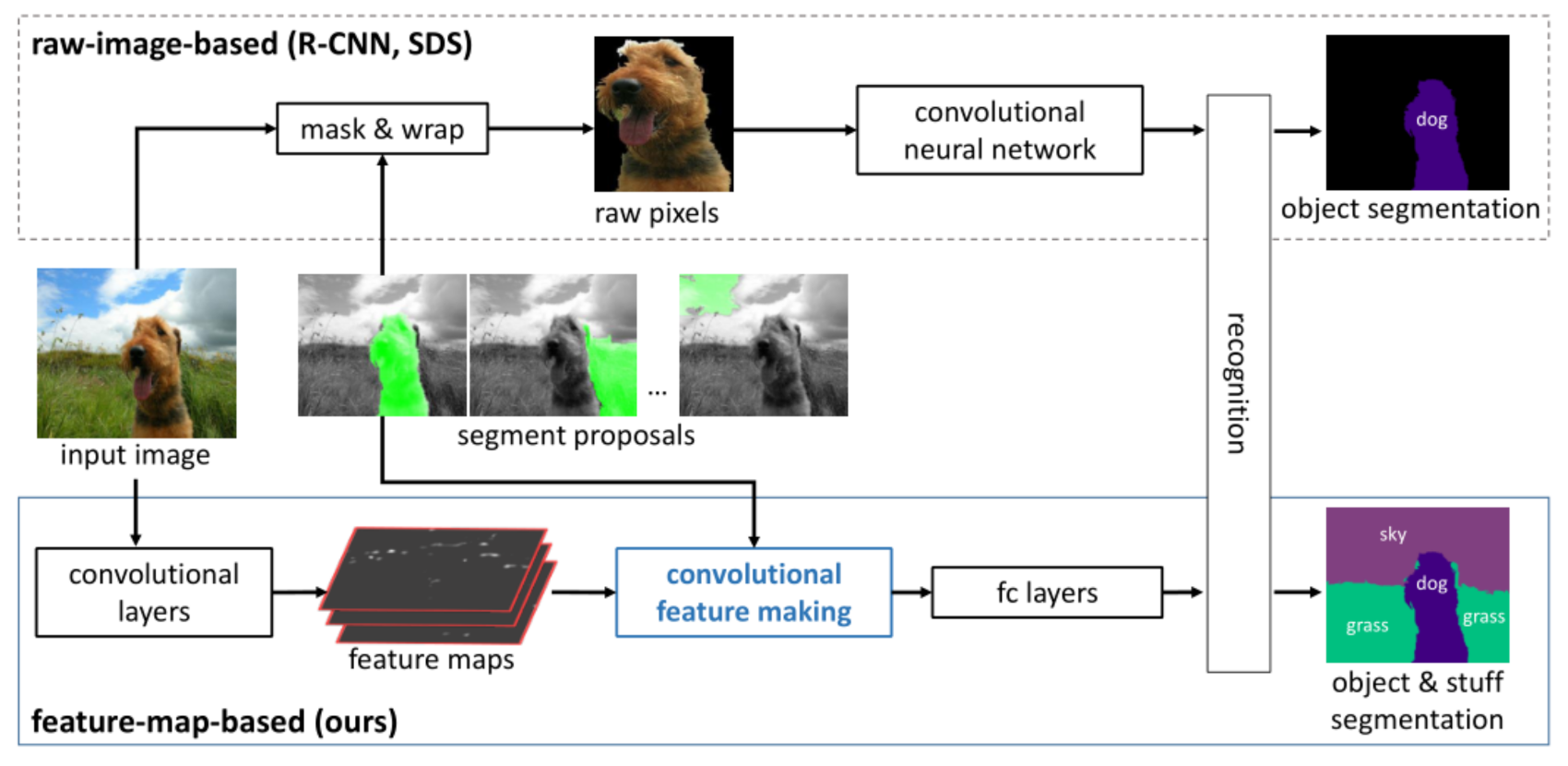
A masking-based method is used to control the region or process of image processing by occluding the selected images to be processed (entirely or partially). A specific image or object for coverage is called a mask. The most important difference between this method and the region proposal-based method is that it does not need to detect the object with the bounding box, since the rectangular frame produced by SDS [64] is very time-consuming. Therefore, Dai et al. proposed to exploit the shape information via convolutional feature masking (CFM) [71]. The proposal segments (e.g., superpixels) are treated as masks on the convolutional feature maps. The CNN features of the segments are directly masked out from these maps via SPPNet [21]. The technical route of CFM and SDS comparison is shown in Figure 12.
In 2015, Facebook Artificial Intelligence (AI) research put forward an instance segmentation method (DeepMask) [72] on the basis of the image masking method, which can divide the image into blocks, determine whether a block contains an object, and accordingly segment the object masks. In the same year, SharpMask [73] was proposed, based on DeepMask, to refine the mask edges further. In 2016, MultipathNet [74] exploited Fast R-CNN to accurately locate objects and combined with the characteristics of DeepMask and SharpMask to further improve the masking accuracy. The relationship between the three can be summarized as (1) DeepMask generates the initial object masks; (2) SharpMask optimizes these masks; and (3) MutiPathNet identifies the objects framed by each mask. In 2019, Lee et al. proposed a simple yet efficient form of anchor-free instance segmentation, called CenterMask, that added a novel spatial attention-guided mask (SAG-Mask) branch to an anchor-free one-stage object detector (FCOS) [31] in the same vein as Mask R-CNN [69].
In this section, we introduced region proposal-based methods and masking-based methods for instance segmentation. In general, the region proposal-based methods produced better accuracies than the masking-based methods. The challenges of instance segmentation still remain for small objects, as well as for efficient end-to-end models and their training schemes.

3.4. Lane Line Segmentation

In traffic scenes, lane lines cover continuous narrow-but-long distances and are pixel-sparse compared with other object categories. It is difficult to segment lane lines and other objects in an image at the same time. Most research treats lane line segmentation as a separate segmentation task. In the early years, there existed many traditional approaches to detect the lane lines using color features [78], edges [79], and other cues, combined with a Huff transform [80] or Kalman filtering [81]. In the latest two years, deep learning-based models have been developed for lane line segmentation. We divide these models into two categories: the two-step method and the end-to-end method.
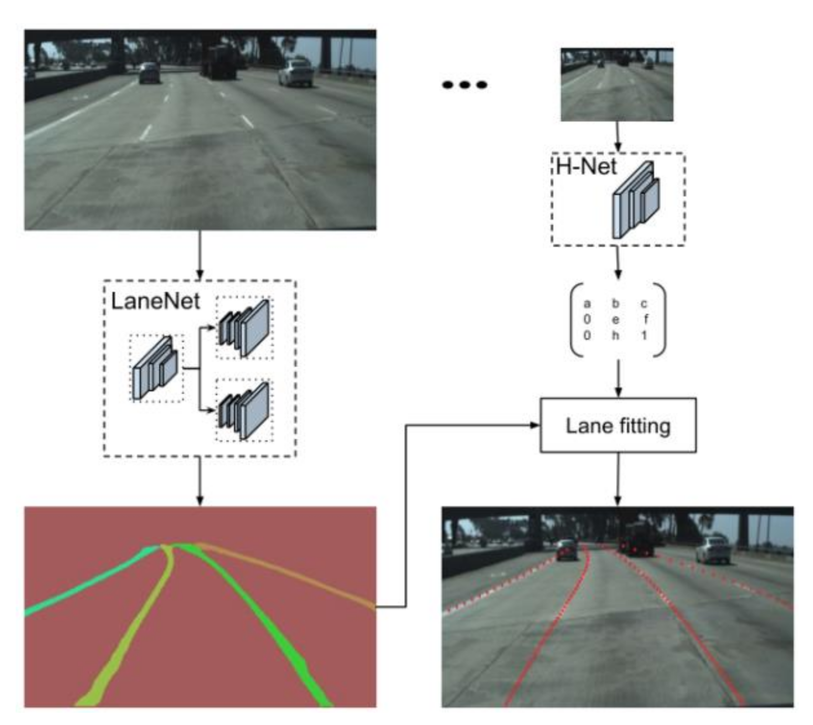
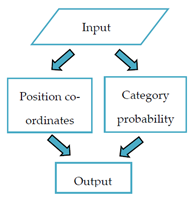
The two-step method usually follows two steps: (1) the lane masks are generated by using deep learning-based semantic segmentation [39,41,82,83]; and (2) the generated lane line masks are fitted by using parametric fitting. For example, H-Net [4] is used to learn the projection matrix, and then the least squares method or the third-order spline curve is used to estimate the lane lines. The end-to-end method considers line fitting as a regression issue and uses a softmax layer at the end of the model to directly return the lane line parameters. Table 5 summarizes the typical work in terms of the dataset, characteristics, core technology and functions.

3.4.1. Two-Step Method

The two-step method accounts for a majority of the deep learning-based lane detection algorithms. They all follow a similar process. The differences between them are given in Table 5. Here, we only describe two representative works: [4] and [11]. The most representative work of the two-step method was LaneNet+H-Net [4], proposed by Neven et al. in 2018. The technical pipeline is shown in Figure 13. They pointed out that the traditional lane detection methods rely on highly specialized and hand-crafted features and are therefore computationally expensive. They pioneered treating the lane detection problem as an instance segmentation problem. They modified E-Net [39] to segment the lane lines and employed the Discriminative Loss Function (DLF) [87] to aggregate the lane line pixels. The segmentation maps of the lane line instances are parametrically output. They also proposed H-Net to learn perspective projection transformation.
Recently, a lane marking semantic segmentation method based on LiDAR and camera fusion was proposed by Yin et al. [93], which was called FusionLane. In order to precisely locate lane lines, semantic segmentation is conducted on the birds-eye view map, converted from LiDAR point clouds. FusionLane uses Deeplab-V3+ [41] to segment the image captured by the camera, and the segmentation result is merged with the point clouds as the input of the network. In addition, they used a recurrent CNN, the long short-term memory (LSTM) network to achieve temporal variation.

3.4.2. End-to-End Method

The problem of the two-step method is that the parameters of the network are not optimized for the task of interest (estimating the lane curvature parameters), but for a proxy task (segmenting the lane markings), resulting in suboptimal performance. The method of end-to-end lane segmentation based on deep learning has fewer corresponding research results. For example, Van et al. [94] proposed a method to train a lane detector in an end-to-end manner, directly regressing the lane parameters. The architecture consisted of two components: a deep network that predicted a segmentation-like weight map for each lane line and a differentiable least squares fitting module that returned the parameters of the best fitting curve in the weighted least squares sense for each map. It realized the backpropagation of the least squares fitting process and directly returned the lane line fitting parameters from end to end. In addition, Qin et al. [96] proposed a form of fast, structure-aware deep lane detection. As shown in Figure 14, they treated the process of lane detection as a row-based selection problem using global features. This clever thinking could significantly impact the computational efficiency.
In this section, we introduced the two-step method and the end-to-end method for lane line recognition. Generally, the two-step method leverages the semantic segmentation models for initial detection and then uses a fitting method to obtain complete lane lines. This type of method is relatively slow, but can detect curved lines. The end-to-end method is relatively fast, but it does not work well for the curved lines.

4. Datasets and Evaluation Criteria

In this section, we summarize the authoritative image datasets used in the autonomous driving research community. We also introduce the primary evaluation criteria for object detection, semantic segmentation, and lane detection.

4.1. Datesets

Table 6 makes a comparison of these datasets in terms of image size, scene weather, and annotation. The annotation gives information about 3D and 2D characteristics, whether the video is supported, and lane line annotation. The datasets are as follows:
  • CamVid [97], or the Cambridge Driving Label Video Database, is the first video collection with semantic labels. There are 32 semantic categories with a total of 710 images. Most of the videos were taken with a fixed-position camera, which partly solved the need for experimental data. However, compared with the datasets released in recent years, there are gaps in the number of labels and the completeness of the labeling;
  • The Karlsruhe Institute of Technology and Toyota Technological Institute (KITTI) [63] dataset was co-founded by the Karlsruhe Institute of Technology in Germany and the Toyota American Institute of Technology. It is one of the most widely used datasets in the field of autonomous driving. It covers object detection, semantic segmentation, and object tracking, among other things. It consists of 389 pairs of stereo images and optical flow maps, a 39.2 km visual ranging sequence, 400 pixel-level segmented maps, and 15,000 traffic scene pictures labeled with bounding boxes;
  • The Cityscapes dataset [62] is comprised of a large, diverse set of stereo video sequences recorded in streets from 50 different cities. It defines 30 visual classes for annotation, which are grouped into eight categories. Of these images, 5000 have high-quality, pixel-level annotations, and 20,000 additional images have coarse annotations. At present, more researchers will use Cityscapes to evaluate algorithm performance in the field of automatic driving;
  • The Mapillary Vistas dataset [98], or Mapillary, is a large-scale, street-level image dataset released in 2017. It has a total of 25,000 high-resolution color images divided into 66 categories, of which 37 categories are specific instance-attached labels. Label annotations for objects can be densely and finely drawn using polygons. It also contains images from all over the world captured under various conditions, including images of different weather, seasons, and times;
  • BDD100K [99] is a large-scale, self-driving dataset with the most diverse content, released by UC Berkeley in 2019. The dataset includes a total of 100,000 videos in complex scenes, such as different weather and times, each about 40 seconds in length. It is divided into 10 categories with about 1.84 million calibration frames. There are a total of 100,000 pictures of high-definition and blurred real driving scenes with different weather, scenes, and times, including 70,000 training sets, 20,000 test sets, and 10,000 validation sets;
  • The ApolloScape open dataset [100], or ApolloScape, was published by Baidu in 2018 for semantic segmentation datasets, specifically for autonomous driving scenarios. Regardless of the amount of data, accuracy of the annotation, or complexity of the scene, it exceeds datasets such as KITTI, Cityscapes, and BDD100K. It contains much larger and richer labeling, including holistic semantic dense point clouds for each site, stereo, per pixel semantic labeling, lane mark labeling, instance segmentation, 3D car instancing, and highly accurate locations for every frame in various driving videos from multiple sites, cities, and daytimes;
  • The Tusimple lane dataset [86] came to be in June 2018, when Tucson held a competition for camera detection using camera image data and later disclosed some of the data. The Tusimple lane dataset consists of 3626 images. The marked lane lines do not distinguish the lane line categories. Each line is synthesized by the coordinates of the point sequence, not a collection of lane line areas;
  • The Caltech dataset [101] is a dataset on lane lines published by the California Institute of Technology in 2008. It includes 1225 road pictures taken at different locations during the day;
  • The CULane dataset [85] is a large-scale, challenging traffic lane detection theoretical research dataset collected by the Chinese University of Hong Kong in 2017. It consists of more than 55 hours of video collected by six different vehicles and 133,235 extracted frames. There are 88,880 training sets, 9675 validation sets, and 34,680 test sets.
  • Currently, the object detection task uses the KITTI dataset as the mainstream. Many excellent models are continuously compared in this dataset. The semantic segmentation task uses the Cityscapes dataset as the mainstream. This dataset has pixel-level annotations for each category in the scene. The annotations are fine and easy to use. The Tusimple lane dataset focuses on the lane line segmentation task with accurate and fine annotation.

4.2. Evaluation Criteria

4.2.1. Evaluation Criteria for Object Detection and Semantic Segmentation

Standard evaluation criteria need to be used to measure the performance of the algorithm on the dataset. Currently, three main aspects are evaluated: runtime, memory consumption, and accuracy. Firstly, the running time of the algorithm is a key indicator that determines whether the algorithm has real-time performance, which mainly depends on the rationality of the algorithm structure and the computing capacity of the running hardware. Secondly, the memory consumption is also a reference value under the same running time and hardware. At present, the evaluation criteria of algorithm performance mainly includes the average recall (AR) [102], average precision (AP) [102], mean average precision(mAP) [102], pixel accuracy (PA) [36], mean accuracy (MA) [36], mean intersection over union (mIoU) [36], and frequency-weighted intersection over union (FWIoU) [36]. Among them, the most commonly used evaluation criteria are the PA, mPA, MA, and mIoU. The specific definitions and calculation formulas are as shown in Equations (1)–(4).
The PA is expressed as the ratio of the pixels marked correctly to the total pixels, and the calculation formula can be written as
P A = i = 1 k P i i i = 1 k T i i
The MA represents the average value of the pixel accuracy of all target categories, and the calculation formula can be written as
M A = 1 k i = 1 k P i i T i
The mIoU represents the average of the degree of coincidence between the predicted area and the actual area, and the calculation formula can be written as
m I o U = 1 k i = 1 k P i i T i + j = 1 k P j i P i i
where k is the number of pixel categories, T i is the total number of pixels of the i-th class, P i i is the total number of pixels with actual type i and prediction type i , and P j i is the total number of pixels with actual type i and prediction type j .
Recently, the three latest evaluation indicators have been proposed by panoptic segmentation [103]: recognition quality (RQ), segmentation quality (SQ), and panoptic segmentation (PQ). RQ represents the accuracy of object recognition for each instance in panoptic segmentation. SQ is simply the average IoU of the matched segments. PQ can be seen as the multiplication of a segmentation quality (SQ) term and a recognition quality (RQ) term:
P Q = p , q I o U p , q T P S e g m e n t a t i o n   Q u a l i t y   S Q × T P T P + 1 2 F P + 1 2 F N R e c o g n i t i o n   Q u a l i t y   R Q
where IoU(p,q) is the category intersection of the true positives (TP), false positives (FP), and false negatives (FN).
The pixel accuracy (PA) is an indispensable evaluation criterion for semantic segmentation which can intuitively judge the number of truly predicted pixels. The mIoU is the most common criterion for segmentation and detection, which efficiently judges the truly predicted area. Comparatively, PA presents a finer evaluation.

4.2.2. Evaluation Criteria for Lane Detection

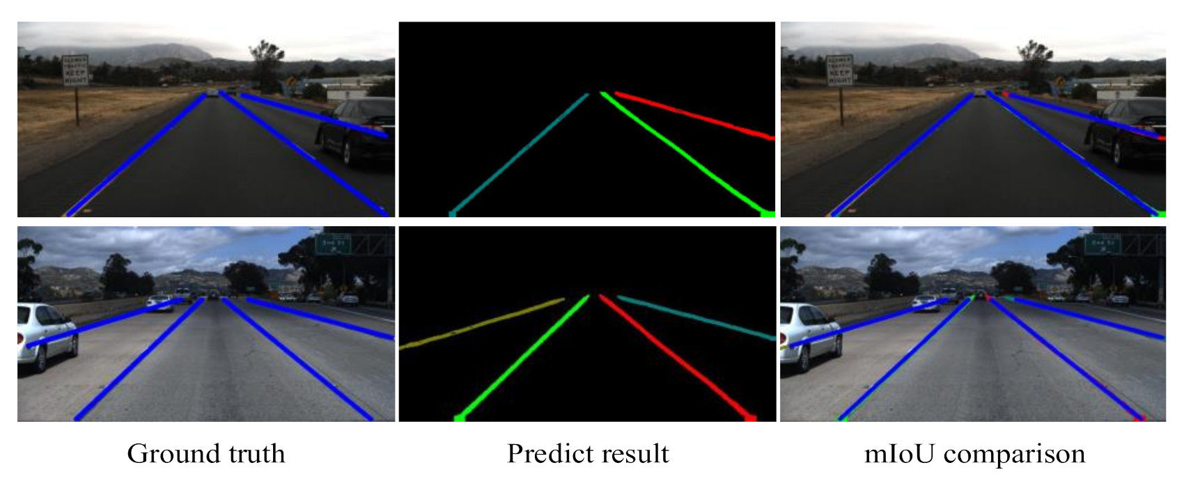
In the Tusimple lane dataset, the accuracy (Acc), false positive rate (FP), and false negative rate (FN) as the evaluation criteria. Besides that, the mean intersection over union (mIoU) is also used for evaluation:
A c c = c l i p C c l i p c l i p S c l i p
F P = F p r e d N p r e d
F N = M p r e d N g t
where C c l i p is the number of lane points predicted correctly in the clip, S c l i p is the total number of points in the clip, F p r e d is the number of wrongly predicted lanes, N p r e d is the number of predicted lanes, M p r e d is the number of missed ground truth lanes, and N g t is the number of all ground truth lanes. Lane markings are regarded as lines with widths equal to 30 pixels, and the mIoUs are calculated. Figure 15 shows an example using the mIoU as the evaluation measure.

5. Performance Comparison

It is difficult to make a comparison of object detection algorithms and lane line segmentation algorithms due to the lack of uniform datasets. This section will only conduct a performance comparison on some of the latest semantic segmentation work, including full-scene semantic segmentation and the instance segmentation.

5.1. Comparison of the Full-Scene Segmentation Algorithms

Table 7 compares representative full-scene semantic segmentation algorithms in terms of the core technology, dataset, mIoU, inference time, and frames per second (fps). It should be noted that the algorithms in Table 6 were all tested on Cityscapes [62]. All results are from the original papers.
It can be seen that Deeplab-V3+ gave the highest mIoU at 82.1%. Due to the integration of Xception, ASPP, dilation convolution, and the encoder and decoder structure, Deeplab-V3+ can aggregate the context information of pixels, perform better inference, and also have better refinement processing for edge pixels. Therefore, DeepLabV3+ reached the best level. Algorithms such as HDC, DANet, FastFCN, and Deeplab-V3 have achieved more than 80% of the mIoU. These algorithms are better than others in terms of processing global image information and the segmentation effect on multiscale objects. PSPNet, Deeplab-V1, DNR, and Deeplab-V2 are relatively fast, with a running speed of less than 1 fps. In general, the algorithms that achieve better results in both speed and accuracy are the algorithms of the PSPNet, FastFCN, and DeepLab series.

5.2. Comparison of the Instance Segmentation Algorithms

Table 8 compares representative instance segmentation algorithms in terms of the year, core technology, datasets, evaluation criteria, and accuracy. All results are from the original papers. The evaluation criteria used in different papers are not uniform, and thus it is difficult to compare them with a unified measure. However, in terms of the actual effect, PANet and CenterMask are superior to their similar methods. Among them, AF pooling in PAN helps to aggregate context information and can improve the segmentation efficiency in cases of object occlusion. SAG-Mask in CenterMask can increase the network’s attention to important features and therefore improve segmentation accuracy.

6. Conclusion Remarks

This paper gives a comprehensive survey of the deep learning-based approaches for scene understanding in autonomous driving. The paper focused on two tasks of scene understanding: object detection and image segmentation. We first briefed the object classification models that formed the basic models of detection and segmentation. Then, we sorted the object detection work into two categories—the two-stage method and the one-stage method—and accordingly reviewed the representative work. According to the particularity of the traffic scene, the image segmentation problem in autonomous driving was deconstructed into full-scene semantic segmentation, instance segmentation, and lane line segmentation. We summarized and compared the up-to-date representative methods used in the three segmentation tasks from four aspects: typical work, characteristics, advantages and disadvantages, and basic frameworks. We also summarized the benchmark datasets and evaluation criteria used in the research community and made a performance comparison on some of the latest works.
Although the research community has made significant progress, there is still a long way to go before a vehicle can recognize the environment like a human. Based on the review above, we believe the following aspects are the challenges in this field.

6.1. 3D Segmentation

The majority of the existing image segmentation work focuses on the two-dimensional segmentation of objects. It would be ideal if we could segment objects in three dimensions. Point clouds generated from LiDAR have obvious advantages for 3D segmentation, compared with image data generated from cameras. Some work has been initiated for this purpose by using LiDAR point clouds or by fusing LiDAR with cameras. However, since point clouds are non-structured data with an irregular format, the challenge goes to how we can model the data by using CNN technology. The main work streams are (1) converting 3D point clouds into 2D images by using view transformation or coordinate transformation, such as in [106,107], (2) voxelizing irregular 3D point clouds into regular 3D tensions and using 3D-CNN [108] to process it, such as in [109,110,111], and (3) direct modeling of the point clouds by using PointNet [112,113] or graph CNNs [114,115].

6.2. Panoptic Segmentation

The majority of the existing vision-based works are designed for the detection or segmentation of particular objects such as roads, pedestrians, vehicles, and so on. It would be ideal if we could segment the scene with complete details, including various object categories such as roads, obstacles, the sky, plants, buildings, and traffic signs. That is called panoramic segmentation, as proposed by Kirillov et al. [103]. In this work, they developed a CNN-based approach to simultaneously segment free space such as the sky, roads, and grass, and obstacles such as pedestrians and cars within a scene. Some algorithms such as DeeperLab [116], JSIS-Net [117], and Panoptic FPN [118] have also emerged for a similar purpose. These algorithms usually use semantic segmentation for free space and instance segmentation for obstacles, and then fuse them together.

6.3. Multitasking Joint Model

The majority of the existing deep learning-based algorithms are designed for a single task. Multiple tasks such as detection and segmentation for various objects request multiple CNN models. This is not applicable for an in-vehicle system that is cost and space sensitive. Thus, whether we can use a single CNN model to fulfill multiple tasks becomes a challenging issue. Some work has been conducted in this area. For example, MultiNet [119] is a multitask model with the encoder–decoder structure, which is capable of detecting obstacles and segmenting roads at the same time. Detection, segmentation, and depth estimation are combined in a single model to identify objects and estimate the depth of the objects in [120].

6.4. Tracking and Behavior Analysis

This paper largely focused on two tasks—object detection and scene segmentation—that are a kind of static understanding of the scene. Actually, tasks like object tracking, behavior analysis, and anomaly detection are also important and even more challenging, since they involve the continuous monitoring and dynamic analysis of single or multiple targets. A recurrent NN with long short-term memory modules for long-term intent prediction of pedestrians was employed in [121]. A method of behavior estimation based on contextual traffic information to recognize and predict lane change intention was proposed in [122]. A visual analytical framework that exploits large amounts of multidimensional road traffic data for anomaly detection was presented in [123].

Author Contributions

Conceptualization, Z.G. and Y.H.; methodology, Z.G. and Y.H.; software, Z.G., Y.H. and X.H.; validation, Z.G. and Y.H.; formal analysis, Z.G., Y.H., X.H., H.W. and B.Z.; investigation, Z.G., Y.H., X.H., H.W. and B.Z.; resources, Z.G. and Y.H.; data curation, Z.G. and Y.H.; writing—original draft preparation, Z.G.; writing—review and editing, Z.G. and Y.H.; visualization, Z.G., Y.H., X.H., H.W. and B.Z.; supervision, Z.G., Y.H., X.H., H.W. and B.Z.; project administration, Y.H.; funding acquisition, Y.H. All authors have read and agreed to the published version of the manuscript.

Funding

This research was funded by the Shanghai Nature Science Foundation of the Shanghai Science and Technology Commission, China, grant number 20ZR1437900 and the National Nature Science Foundation of China, grant number 61374197.

Conflicts of Interest

All authors declare no conflict of interest.

References

  1. Janai, J.; Fatma, G.; Behl, A.; Geiger, A. Computer vision for autonomous vehicles: Problems, datasets and state-of-the-art. Found. Trends Comput. Graph. Vis. 2017, 12, 1–3. [Google Scholar] [CrossRef]
  2. Grigorescu, S.; Trasnea, B.; Cocias, T.; Macesanu, G. A survey of deep learning techniques for autonomous driving. J. Field Robot 2020, 37, 362–386. [Google Scholar] [CrossRef]
  3. Long, S.; He, X.; Yao, C. Scene text detection and recognition: The deep learning era. INT. J. Comput. Vision 2021, 129, 161–184. [Google Scholar] [CrossRef]
  4. Neven, D.; Brabandere, B.-D.; Georgoulis, S.; Proesmans, M. Towards End-to-End Lane Detection: An Instance Segmentation Approach. In Proceedings of the 2018 IEEE Intelligent Vehicles Symposium (IV), Changshu, China, 26–30 June 2018; pp. 286–291. [Google Scholar]
  5. Lecun, Y.; Boser, B.; Denker, J.; Henderson, D.; Howard, R.; Hubbard, W. Backpropagation applied to handwritten zip code recognition. Neural Comput. 1989, 1, 541–551. [Google Scholar] [CrossRef]
  6. Krizhevsky, A.; Sutskever, I.; Hinton, G.E. ImageNet classification with deep convolutional neural networks. In Proceedings of the Advances in Neural Information Processing Systems (NIPS), Lake Tahoe, CA, USA, 3–6 December 2012. [Google Scholar]
  7. Deng, J.; Dong, W.; Socher, R.; Li, L.; Li, K.; Feifei, L. ImageNet: A large-scale hierarchical image database, In Proceedings of the 2009 IEEE Conference on Computer Vision and Pattern Recognition. Miami, FL, USA, 20–25 June 2009; pp. 248–255. [Google Scholar]
  8. Simonyan, K.; Zisserman, A. Very Deep Convolutional Network for Large-Scale Image Recognition. Available online: https://arxiv.org/abs/1409.1556 (accessed on 4 September 2014).
  9. Szegedy, C.; Liu, W.; Jia, Y.; Sermanet, P.; Reed, S.; Anguelov, D.; Erhan, D.; Vanhoucke, V.; Rabinovich, A. Going deeper with convolutions. In Proceedings of the 2015 IEEE Conference on Computer Vision and Pattern Recognition (CVPR), Boston, MA, USA, 7–12 June 2015; pp. 1–9. [Google Scholar]
  10. He, K.; Zhang, X.; Ren, S.; Sun, J. Deep Residual Learning for Image Recognition. In Proceedings of the IEEE Conference on Computer Vision and Pattern Recognition (CVPR), Las Vegas, NV, USA, 26 June–1 July 2016; pp. 770–778. [Google Scholar]
  11. Xie, S.; Girshick, R.; Dollár, P.; Tu, Z.; He, K. Aggregated residual transformations for deep neural networks. In Proceedings of the 2017 IEEE Conference on Computer Vision and Pattern Recognition (CVPR), Honolulu, HI, USA, 21–26 July 2017; pp. 5987–5995. [Google Scholar]
  12. Zhang, X.; Zhou, X.; Lin, M.; Sun, J. ShuffleNet: An Extremely Efficient Convolutional Neural Network for Mobile Devices. In Proceedings of the 2018 IEEE/CVF Conference on Computer Vision and Pattern Recognition, Salt Lake City, UT, USA, 18–23 June 2018; pp. 6848–6856. [Google Scholar]
  13. Ioffe, S.; Szegedy, C. Batch Normalization: Accelerating Deep Network Training by Reducing Internal Covariate Shift. In Proceedings of the International Conference on Machine Learning, Lille, France, 6–11 July 2015; pp. 448–456. [Google Scholar]
  14. Szegedy, C.; Vanhoucke, V.; Ioffe, S.; Shlens, J.; Wojna, Z. Rethinking the Inception Architecture for Computer Vision. In Proceedings of the 2016 IEEE Conference on Computer Vision and Pattern Recognition (CVPR), Las Vegas, NV, USA, 26 June–1 July 2016; pp. 424–437. [Google Scholar]
  15. Szegedy, C.; Ioffe, S.; Vanhoucke, V.; Alemi, A.-A. Inception-v4, Inception-ResNet and the Impact of Residual Connections on Learning. In Proceedings of the Thirty-First AAAI Conference on Artificial Intelligence, San Francisco, CA, USA, 4–9 February 2017; pp. 4278–4284. [Google Scholar]
  16. Chollet, F. Xception: Deep Learning with Depthwise Separable Convolutions. In Proceedings of the IEEE Conference on Computer Vision and Pattern Recognition (CVPR), Honolulu, HI, USA, 21–26 July 2017; pp. 1251–1258. [Google Scholar]
  17. Huang, G.; Liu, Z.; Der Maaten, L.-V.; Weinberger, K.-Q. Densely Connected Convolutional Network. In Proceedings of the 2017 IEEE Conference on Computer Vision and Pattern Recognition (CVPR), Honolulu, HI, USA, 21–26 July 2017; pp. 2261–2269. [Google Scholar]
  18. Zoph, B.; Vasudevan, V.-K.; Shlens, J.; Le, Q.-V. Learning Transferable Architectures for Scalable Image Recognition. In Proceedings of the 2018 IEEE/CVF Conference on Computer Vision and Pattern Recognition, Salt Lake City, UT, USA, 18–23 June 2018; pp. 8697–8710. [Google Scholar]
  19. Hu, J.; Shen, L.; Albanie, S.; Sun, G.; Wu, E. Squeeze-and-excitation networks. IEEE T. Pattern Anal. 2017, 32, 99–113. [Google Scholar]
  20. Girshick, R.; Donahue, J.; Darrell, T.; Malik, J. Rich Feature Hierarchies for Accurate Object Detection and Semantic Segmentation. In Proceedings of the 2014 IEEE Conference on Computer Vision and Pattern Recognition (CVPR), Columbus, OH, USA, 20–23 June 2014; pp. 580–587. [Google Scholar]
  21. He, K.; Zhang, X.; Ren, S.; Sun., J. Intelligence, M. Spatial Pyramid Pooling in Deep Convolutional Network for Visual Recognition. IEEE T. Pattern. Anal. 2015, 37, 1904–1916. [Google Scholar] [CrossRef] [Green Version]
  22. Girshick, R. Fast R-CNN. In Proceedings of the 2015 IEEE International Conference on Computer Vision, Santiago, Chile, 7–13 December 2015; pp. 1440–1448. [Google Scholar]
  23. Ren, S.; He, K.; Girshick, R.; Sun, J. Faster R-CNN: Towards real-time object detection with region proposal networks. In Proceedings of the Conference and Workshop on Neural Information Processing Systems, Long Beach, CA, USA, 4–9 December 2017; pp. 1137–1149. [Google Scholar]
  24. Cai, Z.; Vasconcelos, N. Cascade R-CNN: Delving Into High Quality Object Detection. In Proceedings of the 2018 IEEE/CVF Conference on Computer Vision and Pattern Recognition, Salt Lake City, UT, USA, 18–23 June 2018; pp. 6154–6162. [Google Scholar]
  25. Lin, T.Y.; Dollar, P.; Girshick, R.; He, K.; Hariharan, B.; Belongie, S. Feature pyramid networks for object detection. In Proceedings of the IEEE Conference on Computer Vision and Pattern Recognition, Honolulu, HI, USA, 21–26 July 2017; pp. 2117–2125. [Google Scholar]
  26. Redmon, J.; Divvala, S.; Girshick, R.; Farhadi, A. You Only Look Once: Unified, Real-Time Object Detection. In Proceedings of the 2016 IEEE Conference on Computer Vision and Pattern Recognition (CVPR), Las Vegas, NV, USA, 26 June–1 July 2016; pp. 779–788. [Google Scholar]
  27. Liu, W.; Anguelov, D.; Erhan, D.; Szegedy, C.; Reed, S. SSD: Single shot multibox detector. In European Conference on Computer Vision; Springer: Berlin/Heidelberg, Germany, 2016; pp. 21–37. [Google Scholar]
  28. Lin, T.Y.; Goyal, P.; Girshick, R.; He, K.M.; Dollar, P. Focal loss for dense object detection. IEEE Trans. Pattern Ana. Mach. Intell. 2020, 42, 318–327. [Google Scholar] [CrossRef] [Green Version]
  29. Redmon, J.; Farhadi, A. YOLO9000: Better, Faster, Stronger. In Proceedings of the 2017 IEEE Conference on Computer Vision and Pattern Recognition (CVPR), Honolulu, HI, USA, 21–26 July 2017; pp. 6517–6525. [Google Scholar]
  30. Redmon, J.; Farhadi, A. YOLOv3: An Incremental Improvement. Available online: https://arxiv.org/abs/1804.02767 (accessed on 8 April 2018).
  31. Tian, Z.; Shen, C.; Chen, H.; He, T. FCOS: Fully Convolutional One-Stage Object Detection. In Proceedings of the 2019 IEEE International Conference on Computer Vision, Seoul, Korea, 27 October–2 November 2019; pp. 9627–9636. [Google Scholar]
  32. Yang, Y.; Deng, H. GC-YOLOv3: You Only Look Once with Global Context Block. Electronics 2020, 9, 1235. [Google Scholar] [CrossRef]
  33. Chen, Y.; Han, C.; Wang, N.; Zhang, Z. Revisiting Feature Alignment for One-stage Object Detection. In Proceedings of the 2019 IEEE/CVF Conference on Computer Vision and Pattern Recognition (CVPR), Long Beach, CA, USA, 15–20 June 2019. [Google Scholar]
  34. Duan, K.; Bai, S.; Xie, L.; Qi, H.; Huang, Q.; Tian, Q. Centernet: Keypoint triplets for object detection. In Proceedings of the 2019 IEEE/CVF International Conference on Computer Vision (ICCV), Seoul, Korea, 27 October–2 November 2019. [Google Scholar]
  35. Uijlings, J.; Sande, K.-E.; Gevers, T. Selective Search for Object Recognition. INT. J. Comput. Vision 2013, 104, 154–171. [Google Scholar] [CrossRef] [Green Version]
  36. Long, J.; Shelhamer, E.; Darrell, T. Fully convolutional networks for semantic segmentation. In Proceedings of the IEEE Conference on Computer Vision and Pattern Recognition, Boston, MA, USA, 7–12 June 2015. [Google Scholar]
  37. Badrinarayanan, V.; Cipolla, R. SegNet: A Deep Convolutional Encoder-Decoder Architecture for Image Segmentation. IEEE Trans. Pattern Anal. Mach. Intell. 2017, 39, 2481–2495. [Google Scholar] [CrossRef]
  38. Ronneberger, O.; Fischer, P.; Brox, T. U-net: Convolutional networks for biomedical image segmentation. In International Conference on Medical Image Computing and Computer-Assisted Intervention; Springer: Berlin/Heidelberg, Germany, 2015; pp. 3019–3037. [Google Scholar]
  39. Paszke, A.; Chaurasia, A.; Kim, S.; Culurciello, E. Enet: A deep neural network architecture for real-time semantic segmentation. arXiv 2016, arXiv:1606.02147. [Google Scholar]
  40. Zhao, H.; Shi, J.; Qi, X.; Wang, X.; Jia, J. Pyramid Scene Parsing Network. In Proceedings of the 2017 IEEE Conference on Computer Vision and Pattern Recognition (CVPR), Honolulu, HI, USA, 21–26 July 2017. [Google Scholar]
  41. Chen, L.-C.; Zhu, Y.; Papandreou, G.; Schroff, F.; Adam, H. Encoder-Decoder with Atrous Separable Convolution for Semantic Image Segmentation. In Proceedings of the European Conference on Computer Vision (ECCV), Munich, Germany, 8–14 September 2018; pp. 518–534. [Google Scholar]
  42. Wu, H.; Zhang, J.; Huang, K.; Liang, K. Computer Vision and Pattern Recognition. FastFCN: Rethinking Dilated Convolution in the Backbone for Semantic Segmentation. Available online: https://arxiv.org/abs/1903.11816 (accessed on 28 March 2019).
  43. Khan, A.; Ilyas, T.; Umraiz, M.; Mannan, Z.-I.; Kim, H. CED-Net: Crops and Weeds Segmentation for Smart Farming Using a Small Cascaded Encoder-Decoder Architecture. Electronics 2020, 9, 1602. [Google Scholar] [CrossRef]
  44. Fu, J.; Liu, J.; Tian, H.; Li, Y.; Bao, Y.; Fang, Z.; Lu, H. Dual Attention Network for Scene Segmentation. In Proceedings of the 2019 IEEE/CVF Conference on Computer Vision and Pattern Recognition (CVPR), Long Beach, CA, USA, 15–20 June 2019. [Google Scholar]
  45. Oliveira, G.-L.; Burgard, W.T.; Brox., T. Efficient deep models for monocular road segmentation. In Proceedings of the 2018 IEEE/RSJ International Conference on Intelligent Robots and Systems (IROS), Daejeon, Korea, 9–14 October 2016; pp. 4885–4891. [Google Scholar]
  46. Caltagirone, L.; Bellone, M.; Svensson, L.; Wahde, M.J.R.; Systems, A. LIDAR-Camera Fusion for Road Detection Using Fully Convolutional Neural Network. Robot. Auton. Syst. 2019, 111, 125–131. [Google Scholar] [CrossRef] [Green Version]
  47. Munozbulnes, J.; Fernandez, C.-I.; Parra, I.; Fernandezllorca, D.; Sotelo, M.-A. Deep fully convolutional network with random data augmentation for enhanced generalization in road detection. In Proceedings of the 2017 IEEE 20th International Conference on Intelligent Transportation Systems (ITSC), Yokohama, Japan, 16–19 October 2017; pp. 366–371. [Google Scholar]
  48. Luc, P.; Couprie, C.; Chintala, S.; Verbeek, J. Semantic Segmentation using Adversarial Network. Available online: https://arxiv.org/abs/1412.7062 (accessed on 22 December 2014).
  49. Yu, Y.; Koltun, V. Multi-scale context aggregation by dilated convolutions. Available online: https://arxiv.org/abs/1511.07122 (accessed on 23 November 2015).
  50. Chen, L.-C.; Papandreou, G.; Murphy, K.; Yuille, A.L. DeepLab: Semantic Image Segmentation with Deep Convolutional Nets, Atrous Convolution, and Fully Connected CRFs. IEEE Trans. Pattern Anal. Mach. Intell. 2018, 40, 834–848. [Google Scholar] [CrossRef]
  51. Chen, L.-C.; Papandreou, G.; Schroff, F.; Adam, H. Rethinking atrous convolution for semantic image segmentation. Available online: https://arxiv.org/abs/1706.05587 (accessed on 17 June 2017).
  52. Zheng, S. Conditional Random Fields as Recurrent Neural Network. In Proceedings of the 2015 IEEE International Conference on Computer Vision, Santiago, Chile, 7–13 December 2015; pp. 1529–1537. [Google Scholar]
  53. Yu, F.; Koltun, V.; Funkhouser, T. Dilated Residual Network. In Proceedings of the 2017 IEEE Conference on Computer Vision and Pattern Recognition (CVPR), Honolulu, HI, USA, 21–26 July 2017; pp. 636–644. [Google Scholar]
  54. Wang, P.; Chen, P.; Yuan, Y.; Liu, D.; Huang, Z.; Hou, X. Understanding Convolution for Semantic Segmentation. In Proceedings of the 2018 IEEE Winter Conference on Applications of Computer Vision (WACV), Lake Tahoe, CA, USA, 12–15 May 2018; pp. 1451–1460. [Google Scholar]
  55. Ladicky, L.; Russell, C.; Kohli, P.; Torr, P. Associative hierarchical CRFs for object class image segmentation. In Proceedings of the 2009 IEEE International Conference on Computer Vision, Kyoto, Japan, 29 September–2 October 2009; pp. 739–746. [Google Scholar]
  56. Shotton, J.; Winn, J.; Rother, C.; Criminisi, A. TextonBoost for Image Understanding: Multi-Class Object Recognition and Segmentation by Jointly Modeling Texture, Layout, and Context. INT. J. Compute. Vision 2009, 81, 2–23. [Google Scholar] [CrossRef] [Green Version]
  57. Farabet, C.; Couprie, C.; Najman, L.; Lecun, Y. Learning Hierarchical Features for Scene Labeling. IEEE T. Pattern Anal. 2013, 35, 1915–1929. [Google Scholar]
  58. Gupta, S.; Girshick, R.; Arbelaez, P.; Malik, J. Learning Rich Features from RGB-D Images for Object Detection and Segmentation. In European Conference on Computer Vision; Springer: Zurich, Switzerland, 2014; pp. 345–360. [Google Scholar]
  59. Lin, G.; Milan, A.; Shen, C.; Reid, I. RefineNet: Multi-path Refinement Network for High-Resolution Semantic Segmentation. In Proceedings of the 2017 IEEE Conference on Computer Vision and Pattern Recognition (CVPR), Honolulu, HI, USA, 21–26 July 2017; pp. 5168–5177. [Google Scholar]
  60. Ren, G.; Dai, T.; Barmpoutis, P.; Stathaki, T. Salient Object Detection Combining a Self-Attention Module and a Feature Pyramid Network. Electronics 2020, 9, 1702. [Google Scholar] [CrossRef]
  61. Krahenbuhl, P.; Koltun, V. Efficient Inference in Fully Connected CRFs with Gaussian Edge Potentials. In Proceedings of the Advances in Neural Information Processing Systems (NIPS), Granada, Spain, 12–15 December 2011; pp. 109–117. [Google Scholar]
  62. Cordts, M. The Cityscapes Dataset for Semantic Urban Scene Understanding. In Proceedings of the 2016 IEEE Conference on Computer Vision and Pattern Recognition (CVPR), Las Vegas, NV, USA, 26 June–1 July 2016; pp. 3213–3223. [Google Scholar]
  63. Geiger, A.; Lenz, P.; Stiller, C. Vision meets robotics: The KITTI dataset. Int. J. Rob. Res 2013, 32, 1231–1237. [Google Scholar] [CrossRef] [Green Version]
  64. Hariharan, B.; Arbelaez, P.; Girshick, R.; Malik, J. Simultaneous Detection and Segmentation. In European Conference on Computer Vision; Springer: Zurich, Switzerland, 2014; pp. 297–312. [Google Scholar]
  65. Hariharan, B.; Arbelaez, P.; Girshick, R.; Malik, J. Hypercolumns for object segmentation and fine-grained localization. In Proceedings of the 2015 IEEE Conference on Computer Vision and Pattern Recognition (CVPR), Boston, MA, USA, 7–12 June 2015; pp. 447–456. [Google Scholar]
  66. Dai, J.; He, K.; Sun, J. Instance-Aware Semantic Segmentation via Multi-task Network Cascades. In Proceedings of the 2016 IEEE Conference on Computer Vision and Pattern Recognition (CVPR), Las Vegas, NV, USA, 26 June–1 July 2016; pp. 3150–3158. [Google Scholar]
  67. Dai, J.; He, K.; Li, Y.; Ren, S.; Sun, J. Instance-Sensitive Fully Convolutional Network. In European Conference on Computer Vision; Springer: Berlin/Heidelberg, Germany, 2016; pp. 534–549. [Google Scholar]
  68. Li, Y.; Qi, H.; Dai, J.; Ji, X.; Wei, Y. Fully Convolutional Instance-Aware Semantic Segmentation. In Proceedings of the 2017 IEEE Conference on Computer Vision and Pattern Recognition (CVPR), Honolulu, HI, USA, 21–26 July 2017; pp. 4438–4446. [Google Scholar]
  69. He, K.; Gkioxari, P.; Dollar, P.; Girshick, R. Mask R-CNN. In Proceedings of the 2017 IEEE Conference on Computer Vision and Pattern Recognition (CVPR), Honolulu, HI, USA, 21–26 July 2017; pp. 2980–2988. [Google Scholar]
  70. Liu, S.; Qi, L.; Qin, H.; Shi, J.; Jia, J. Path Aggregation Network for Instance Segmentation. In Proceedings of the 2018 IEEE/CVF Conference on Computer Vision and Pattern Recognition, Salt Lake City, UT, USA, 18–23 June 2018; pp. 8759–8768. [Google Scholar]
  71. Dai, J.; He, K.; Sun, J. Convolutional feature masking for joint object and stuff segmentation. In Proceedings of the 2015 IEEE Conference on Computer Vision and Pattern Recognition (CVPR), Boston, MA, USA, 7–12 June 2015; pp. 3992–4000. [Google Scholar]
  72. Pinheiro, P.-O.; Collobert, R.; Dollar, P. Learning to segment object candidates. In NIPS’15: Proceedings of the 28th International Conference on Neural Information Processing Systems; Association for Computing Machinery (ACM): New York, NY, USA, 2018; pp. 1990–1998. [Google Scholar]
  73. Pinheiro, P.-O.; Lin, T.; Collobert, R.; Dollar, P. Learning to Refine Object Segments. In European Conference on Computer Vision; Springer: Berlin/Heidelberg, Germany, 2016; pp. 75–91. [Google Scholar]
  74. Zagoruyko, S. A MultiPath Network for Object Detection. IEEE Conf. Compute. Vision. Pattern Recognit. 2016, 214–223. [Google Scholar]
  75. Hu, R.; Dollar, P.; He, K.; Darrell, T.; Girshick, R. Learning to Segment Every Thing. In Proceedings of the 2018 IEEE/CVF Conference on Computer Vision and Pattern Recognition, Salt Lake City, UT, USA, 18–23 June 2018; pp. 4233–4241. [Google Scholar]
  76. Lee, Y.; Park, J. CenterMask: Real-Time Anchor-Free Instance Segmentation. Available online: https://arxiv.org/abs/1911.06667 (accessed on 15 November 2019).
  77. Arbelaez, P.; Ponttuset, J.; Barron, J.; Marques, F.; Malik, J. Multiscale Combinatorial Grouping. In Proceedings of the IEEE Conference on Computer Vision and Pattern Recognition Workshops, Columbus, OH, USA, 23–28 June 2014; pp. 328–335. [Google Scholar]
  78. Chiu, K.; Lin, S. Lane detection using color-based segmentation. In Proceedings of the 2005 IEEE Intelligent Vehicles Symposium (IV), Las Vegas, NV, USA, 6–8 June 2005; pp. 706–711. [Google Scholar]
  79. Lopez, A.-M.; Serrat, J.; Canero, C.; Lumbreras, F. Robust lane markings detection and road geometry computation. INT J. Auto. Tech-Kor. 2010, 11, 395–407. [Google Scholar] [CrossRef]
  80. Liu, G.; Worgotter, F.; Markelic, I. Combining Statistical Hough Transform and Particle Filter for robust lane detection and tracking. In Proceedings of the 2010 IEEE Intelligent Vehicles Symposium (IV), San Diego, CA, USA, 21–24 June 2010; pp. 993–997. [Google Scholar]
  81. Danescu, R.; Nedevschi, S. Probabilistic Lane Tracking in Difficult Road Scenarios Using Stereovision. IEEE Trans. Pattern Anal. Mach. Intell. 2009, 10, 272–282. [Google Scholar] [CrossRef]
  82. Romera, E.; Alvarez, J.-M.; Bergasa, L.-M.; Arroyo, R. Efficient ConvNet for real-time semantic segmentation. In Proceedings of the 2010 IEEE Intelligent Vehicles Symposium (IV), Los Angeles, CA, USA, 21–26 June 2017; pp. 1789–1794. [Google Scholar]
  83. Luc, P.; Couprie, C.; Chintala, S.; Verbeek, J. Semantic Segmentation using Adversarial Network. Proc. Adv. Neural Inf. Process. Syst. 2016, 4, 216–228. [Google Scholar]
  84. Lee, S.; Kim, J.; Yoon, J.S.; Shin, S.; Bailo, O.; Kim, N.; Lee, T.-H.; Hong, S.H.; Han, S.-H.; Kweon, I.S. VPGNet: Vanishing Point Guide Network for Lane and Road Marking Detection and Recognition. In Proceedings of the 2015 IEEE International Conference on Computer Vision, Venice, Italy, 22–29 October 2017; pp. 1965–1973. [Google Scholar]
  85. Pan, X.; Shi, J.; Luo, P.; Wang, X.; Tang, X. Spatial As Deep: Spatial CNN for Traffic Scene Understanding. In Proceedings of the National Center of Artificial Intelligence-NCAI, Islamabad, Pakistan; 2018; pp. 7276–7283. [Google Scholar]
  86. The tuSimple lane challenge. Available online: http://ben-chmark.tusimple.ai/ (accessed on 4 July 2018).
  87. Brabandere, B.-D.; Neven, D.; Recognition, P. Semantic Instance Segmentation with a Discriminative Loss Function. Available online: https://arxiv.org/abs/1708.02551 (accessed on 8 August 2017).
  88. Wang, Z.; Ren, W.; Qiu, Q. LaneNet: Real-Time Lane Detection Network for Autonomous Driving. Available online: https://arxiv.org/abs/1807.01726 (accessed on 4 July 2018).
  89. Ghafoorian, M.; Nugteren, C.; Baka, N.; Booij, O. EL-GAN: Embedding Loss Driven Generative Adversarial Network for Lane Detection. Available online: https://arxiv.org/abs/1806.05525 (accessed on 5 July 2018).
  90. Ko, Y.; Jun, J.; Ko, D. Key Points Estimation and Point Instance Segmentation Approach for Lane Detection. Available online: https://arxiv.org/abs/2002.06604 (accessed on 16 February 2020).
  91. Jung, J.; Bae, S.-H. Real-time road lane detection in Urban areas using LiDAR data. Electronics 2018, 7, 325–337. [Google Scholar] [CrossRef] [Green Version]
  92. Naver Map. Available online: https://map.naver.com (accessed on 1 July 2018).
  93. Schlosser, J.; Chow, C.-K.; Kira, Z. Fusing LIDAR and images for pedestrian detection using convolutional neural network. In Proceedings of the 2016 IEEE International Conference on Robotics and Automation (ICRA), Stockholm, Sweden, 16–21 May 2016; pp. 2198–2205. [Google Scholar]
  94. Van Gansbeke, W.; De Brabandere, B.; Neven, D.; Proesmans, M.; Van Gool, L. End-to-end Lane Detection through Differentiable Least-Squares Fitting. In Proceedings of the 2019 IEEE International Conference on Computer Vision, Seoul, Korea, 27 October–2 November 2019; pp. 4213–4225. [Google Scholar]
  95. Garnett, N.; Cohen, R.; Peer, T.; Lahav, R.; Levi, D. 3D-LaneNet: End-to-End 3D Multiple Lane Detection. In Proceedings of the 2019 IEEE International Conference on Computer Vision, Seoul, Korea, 27 October–2 November 2019; pp. 2921–2930. [Google Scholar]
  96. Qin, Z.; Wang, H.; Li, X. Ultra Fast Structure-aware Deep Lane Detection. In European Conference on Computer Vision; Springer: Glasgow, UK, 2020; pp. 276–291. [Google Scholar]
  97. Brostow, G.-J.; Shotton, J.; Fauqueur, J.; Cipolla, R. Segmentation and Recognition Using Structure from Motion Point Clouds. In European Conference on Computer Vision; Springer: Verlag, Germany, 2018; pp. 534–549. [Google Scholar]
  98. Neuhold, G.; Ollmann, T.; Bulo, S.-R. The Mapillary Vistas Dataset for Semantic Understanding of Street Scenes. In Proceedings of the 2017 IEEE International Conference on Computer Vision, Venice, Italy, 22–29 October 2017; pp. 5000–5009. [Google Scholar]
  99. Yu, F.; Chen, H.; Wang, X.; Xian, W.; Chen, Y.; Liu, F. Bdd100k: A diverse driving dataset for heterogeneous multitask learning. arXiv 2019, arXiv:1805.04687. [Google Scholar]
  100. Huang, X.; Cheng, X.; Geng, Q. The ApolloScape Dataset for Autonomous Driving. In Proceedings of the 2018 IEEE/CVF Conference on Computer Vision and Pattern Recognition, Salt Lake City, UT, USA, 18–23 June 2018; pp. 954–960. [Google Scholar]
  101. Aly, M. Real time detection of lane markers in urban streets. In Proceedings of the 2008 Intelligent Vehicles Symposium, Eindhoven, The Netherlands, 4–6 June 2008; pp. 7–12. [Google Scholar]
  102. Turpin, A.; Scholer, F. User performance versus precision measures for simple search tasks. In Proceedings of the 29th annual international ACM SIGIR conference on Research and development in information retrieval, Seattle, WA, USA, 6–11 August 2006; pp. 11–18. [Google Scholar]
  103. Kirillov, A.; He, K.; Girshick, R. Panoptic Segmentation. In Proceedings of the IEEE/CVF Conference on Computer Vision and Pattern Recognition (CVPR), Long Beach, CA, USA, 15–20 June 2019; pp. 9404–9413. [Google Scholar]
  104. Everingham, M.; Van Gool, L.; Williams, C.K.I.; Winn, J. The Pascal Visual Object Classes (VOC) Challenge. Int. J. Comput. Vis. 2010, 88, 303–338. [Google Scholar] [CrossRef] [Green Version]
  105. Lin, T.-Y.; Maire, M.; Belongie, S.; Hays, J.; Perona, P.; Ramanan, D.; Dollár, P.; Zitnick, C.L. Microsoft COCO: Common objects in context. In European Conference on Computer Vision; Springer: Berlin/Heidelberg, Germany, 2014; pp. 740–755. [Google Scholar]
  106. Kato, H.; Ushiku, Y.; Harada, T. Neural 3d mesh renderer. In Proceedings of the 2018 IEEE/CVF Conference on Computer Vision and Pattern Recognition, Salt Lake City, UT, USA, 18–23 June 2018; pp. 3907–3916. [Google Scholar]
  107. Asvadi, A.; Garrote, L.; Premebida, C.; Peixoto, P.; Nunes, U.J. Multimodal vehicle detection: Fusing 3D-LIDAR and color camera data. Pattern. Recogn. Lett. 2017, 115, 20–29. [Google Scholar] [CrossRef]
  108. Ji, S.; Xu, W.; Yang, M. 3D Convolutional Neural Network for Human Action Recognition. IEEE T. Pattern. Anal. 2013, 35, 221–231. [Google Scholar] [CrossRef] [Green Version]
  109. Zhou, Y.; Tuzel, O. VoxelNet: End-to-End Learning for Point Cloud Based 3D Object Detection. In Proceedings of the 2018 IEEE/CVF Conference on Computer Vision and Pattern Recognition, Salt Lake City, UT, USA, 21–23 June 2018; pp. 4490–4499. [Google Scholar]
  110. Chen, Y.; Liu, S.; Shen, X.; Jia, J. Fast Point R-CNN. In Proceedings of the 2019 IEEE International Conference on Computer Vision, Seoul, Korea, 27 October–3 November 2019; pp. 9775–9784. [Google Scholar]
  111. Charles, R.-Q.; Su, H.; Kaichun, M.; Guibas, L.-J. Volumetric and Multi-view CNNs for Object Classification on 3D Data. In Proceedings of the 2016 IEEE Conference on Computer Vision and Pattern Recognition (CVPR), Las Vegas, NV, USA, 26 June–1 July 2016; pp. 5648–5656. [Google Scholar]
  112. Charles, R.-Q.; Su, H.; Kaichun, M.; Guibas, L.-J. PointNet: Deep Learning on Point Sets for 3D Classification and Segmentation. In Proceedings of the 2017 IEEE Conference on Computer Vision and Pattern Recognition (CVPR), Honolulu, HI, USA, 21–26 July 2017; pp. 77–85. [Google Scholar]
  113. Wang, Z.; Jia, K. Frustum ConvNet: Sliding Frustums to Aggregate Local Point-Wise Features for Amodal 3D Object Detection. In Proceedings of the IEEE/CVF Conference on Computer Vision and Pattern Recognition (CVPR), Long Beach, CA, USA, 15–20 June 2019; pp. 6399–6408. [Google Scholar]
  114. Wang, Y.; Sun, Y.; Liu, Z.; Sarma, S.-E.; Bronstein, M.-M.; Solomon, J.M. Dynamic Graph CNN for Learning on Point Clouds. ACM Trans. Graphic 2019, 38, 146–159. [Google Scholar] [CrossRef] [Green Version]
  115. Landrieu, L.; Simonovsky, M. Large-Scale Point Cloud Semantic Segmentation with Superpoint Graphs. In Proceedings of the 2018 IEEE/CVF Conference on Computer Vision and Pattern Recognition, Salt Lake City, UT, USA, 18–23 June 2018; pp. 4558–4567. [Google Scholar]
  116. Yang, T.-J.; Collins, M.D.; Zhu, Y.; Hwang, Y.-Y.; Liu, T.; Zhang, X.; Sze, V.; Papendreou, G.; Chen, L.-C. DeeperLab: Single-Shot Image Parser. Available online: https://arxiv.org/abs/1902.05093 (accessed on 11 February 2019).
  117. De Geus, D.; Meletis, P. Panoptic segmentation with a joint semantic and instance segmentation network. Available online: https://arxiv.org/abs/1809.02110 (accessed on 9 September 2018).
  118. Kirillov, A.; Girshick, R.; He, K.; Dollar, P. Panoptic Feature Pyramid Network. In Proceedings of the IEEE/CVF Conference on Computer Vision and Pattern Recognition (CVPR), Long Beach, CA, USA, 15–20 June 2019; pp. 6399–6408. [Google Scholar]
  119. Teichmann, M.; Weber, M.; Zollner, M.; Cipolla, R.; Urtasun, R. MultiNet: Real-time Joint Semantic Reasoning for Autonomous Driving. In Proceedings of the 2018 Intelligent Vehicles Symposium, Changshu, Suzhou, China, 26–30 June 2018; pp. 1013–1020. [Google Scholar]
  120. Chen, L.; Yang, Z.; Ma, J.; Luo, Z. Driving Scene Perception Network: Real-Time Joint Detection, Depth Estimation and Semantic Segmentation. In Proceedings of the 2018 IEEE Winter Conference on Applications of Computer Vision (WACV), Lake Tahoe, CA, USA, 12–15 March 2018; pp. 1283–1291. [Google Scholar]
  121. Saleh, K.; Hossny, M.; Nahavandi, S. Intent Prediction of Pedestrians via Motion Trajectories Using Stacked Recurrent Neural Network. IEEE T. Intell. Transp. 2018, 3, 414–424. [Google Scholar] [CrossRef]
  122. Zhang, J.; Xu, Y.; Ni, B.; Duan, Z. Geometric Constrained Joint Lane Segmentation and Lane Boundary Detection. In Proceedings of the European Conference on Computer Vision (ECCV), Munich, Germany, 8–14 September 2018; pp. 502–518. [Google Scholar]
  123. Riveiro, M.; Lebram, M.; Elmer, M. Anomaly Detection for Road Traffic: A Visual Analytics Framework. IEEE Trans. Intell. Transp. Syst. 2017, 18, 2260–2270. [Google Scholar] [CrossRef]
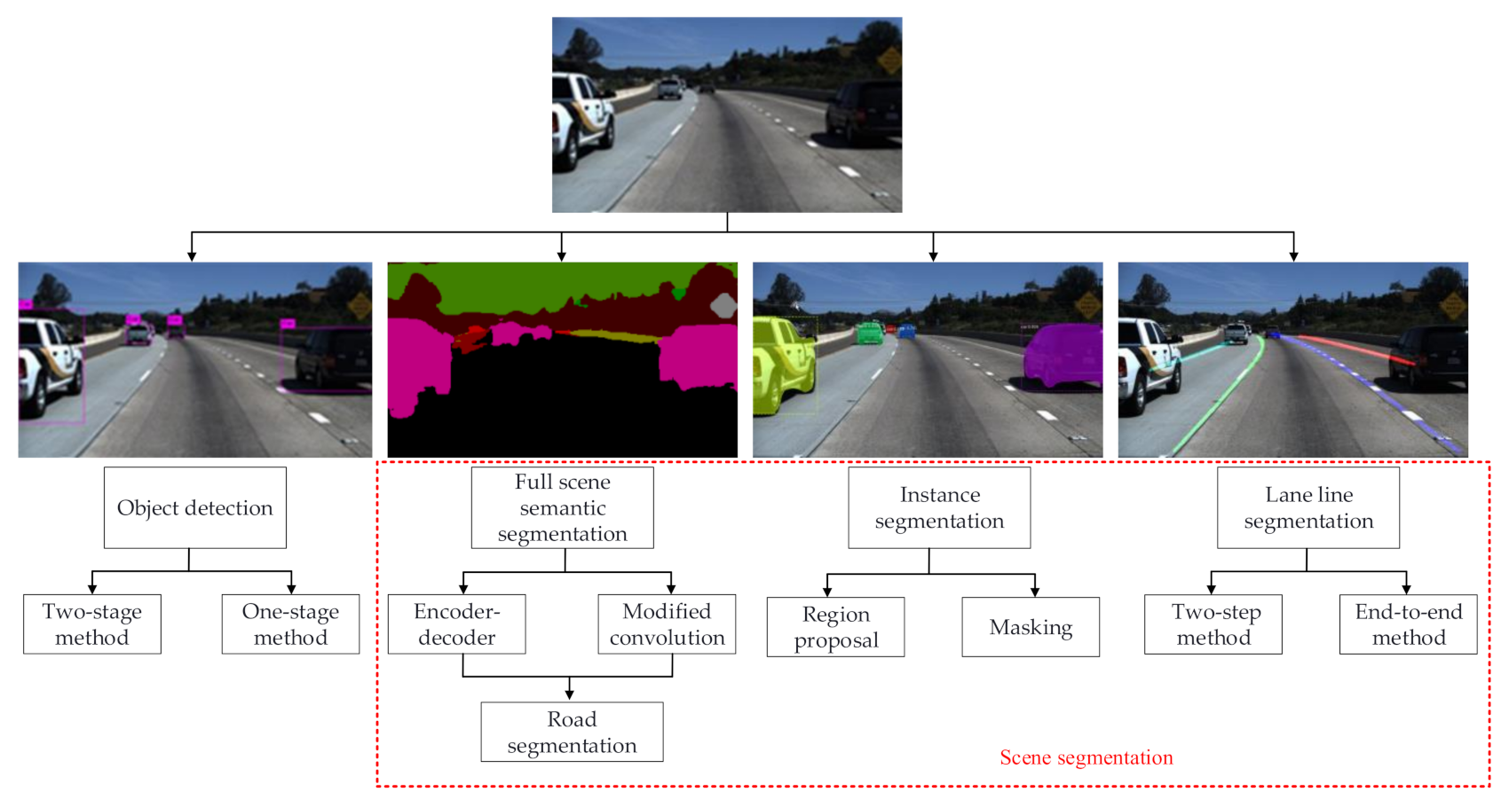
Figure 1. The overall framework of this paper.
Electronics 10 00471 g001
Figure 2. The process of R-CNN detection: (1) input an image; (2) generate around 2000 bottom-up region proposals; (3) extract features for each proposal using a large number of Convolutional Neural Networks (CNNs); and (4) classify each region using class-specific linear Support Vector Machine (SVMs) (Figure reproduced in [20]).
Electronics 10 00471 g002
Figure 3. An illustration of the SegNet architecture (Figure reproduced from [37]).
Electronics 10 00471 g003
Figure 4. An illustration of the dilated convolution architecture. This can be summarized as the relationship between the dilated number i and the receptive field area F, expressed as F i = ( 2 × i 1 ) × ( 2 × i 1 ) (Figure reproduced from [48]).
Electronics 10 00471 g004
Figure 5. The framework of DeepLab-V3+ architecture. Multiscale downsampling is performed through an atrous pyramid convolution to obtain 1/16 feature maps at the encoding stage. The decoding stage consists of three parts: F1, F2, and F3. In F1, the features extracted at the encoding stage are upsampled four times. In F2, the feature at the same scale as F1 is additionally extracted at the encoding stage, and 1 × 1 convolution is performed to reduce the number of channels to obtain F2. In F3, the respective feature maps of F1 and F2 are connected, and 3 × 3 convolution fine-tuning features are performed, and the segmentation map by upsampling four times is output.
Electronics 10 00471 g005
Figure 6. Visualization results with the Cityscapes dataset.
Electronics 10 00471 g006
Figure 7. Segmentation results for road segmentation extracted from the KITTI benchmark. Green corresponds to correct segmentation, red to false negative detection, and blue to false positive detection (Figure reproduced from the papers).
Electronics 10 00471 g007
Figure 8. The technical process of simultaneous detection and segmentation (SDS). Multiscale Combinatorial Grouping (MCG) [77] is used to extract region proposals. A CNN extracts the features in the region and classifies them with SVM, then finally refines the segmentation effect. (Figure reproduced from [64]).
Electronics 10 00471 g008
Figure 9. An illustration of the Mask R-CNN architecture. The technical processes are as follows: (1) feature extraction by using ResNet [10] and an FPN [25]; (2) ROI generation by a region proposal network (RPN) on the last layer of the convolution feature map [23]; (3) an RoI Align layer making each suggestion window generate a fixed-size feature map; and (4) the generation three output vectors, the first being the softmax classification, the second being the coordinate regression of each class, and the third being the ROI segmentation mask.
Electronics 10 00471 g009
Figure 10. An illustration of the PAN architecture. (a) FPN backbone; (b) Bottom-up path augmentation; (c) Adaptive feature pooling; (d) Boxbranch; (e) Fully-connected fusion. (Figure reproduced from [70]).
Electronics 10 00471 g010
Figure 11. Visualization results of the PAN [70].
Electronics 10 00471 g011
Figure 12. The technical route of convolutional feature masking (CFM) and simultaneous detection and segmentation (SDS) comparison. (Figure reproduced from [71]).
Electronics 10 00471 g012
Figure 13. The technical route of LaneNet. (Figure reproduced from [4]).
Electronics 10 00471 g013
Figure 14. Illustration of the row-based selecting problem.
Electronics 10 00471 g014
Figure 15. Evaluation based on the mean intersection over union (mIoU). In the third column, the blue lines are the ground truth and other colors are the predicted results of each line.
Electronics 10 00471 g015
Table 1. Summary of classic convolutional neural network (CNN) models for classification.
Classical
Methods
YearBackgroundAlgorithm
Characteristics
Contributions
LetNet [5]1998This classical CNN was originally proposed for character recognition5-layer CNN
Simple architecture,
less parameters
The basic structure of the modern CNN
AlexNet [6]2012The championship in ILSVRC 2012layer CNN
Use Relu and Dropout functions for reducing overfitting.
It brought the research boom of deep learning today
VGGNet [7]2014The championship of location project in ILSVRC 2014Repeatedly superimposing the convolutional layer and the pooling layerThe relationship between the depth of the CNN and the performance of the model is studied
GoogLeNet [9]2014The championship of classification
project in ILSVRC 2014
Inception V1 moduleEfficient use of 1 × 1, 3 × 3, and 5 × 5 convolution. The efficiency reached the human level and subsequently developed into V2 [13], V3 [14], V4 [15], and Xception [16].
ResNet [10]2015The championship in ILSVRC 2015Residual UintLearning the difference between the input and output. Subsequently, ResNeXt [11] was proposed by combining it with Inception.
DenseNet [17]2016Proposed by Gao et al.DenseBlockRealization of reuse between features
NASNet [18]2017Proposed by GoogleResNet + InceptionCombination of previous network Structures
ShuffleNet [12]2017Proposed by Zhang et al.Channel shuffleImproving network information blocking
SeNet [19]2017The championship in ILSVRC 2017Squeeze and excitation moduleThe relationship between the feature
channels is studied
Table 2. Comparison of deep learning-based approaches for object detection.
Method CategoryTypical WorkCharacteristicsAdvantages and DisadvantagesBasic Framework
Two-stageR-CNN [20]
SPPNet [21]
Fast R-CNN [22]
Faster R-CNN [23]
Cascade R-CNN [24]
FPN [25]
(1)
Propose a large number of regions by selective searching;
(2)
Detect objects in the region proposals;
(3)
Change the way of extracting features from samples and solve the problem that a CNN model is hard to be trained with a small number of samples.
Advantages:
High detection accuracy
 
Disadvantages:
Multistage pipeline training
Slow object detection
Electronics 10 00471 i001
One-stageYOLO-V1 [26]
SSD [27]
RetinaNet [28]
YOLO-V2 [29]
YOLO-V3 [30]
FCOS [31]
GC-YOLOv3 [32]
AlignDet [33]
CenterNet [34]
(1)
No region proposal stage and processing of the entire picture during training and prediction;
(2)
End-to-end detection with a single CNN model so it can directly output object positions and categories from the input image.
Advantages:
Fast object detection
 
Disadvantages:
Relatively low detection accuracy
Electronics 10 00471 i002
Table 3. Comparison of deep learning-based approaches for full-scene semantic segmentation.
Method CategoryTypical WorkCharacteristicsCore Technology
and Functions
Basic FrameworkRoad Segmentation
Encoder–
Decoder
FCN [36]
SegNet [37]
U-Net [38]
ENet [39]
PSPNet [40]
Deeplab-V3+ [41]
Fast FCN [42]
CED-Net [43]
DANet [44]
End-to-end dense pixel output
The pyramid pooling module can ensure global information integrity
(1)
Deconvolution:
Upsampling;
(2)
UnPooling:
Increasing the resolution of the feature map;
(3)
Bilinear interpolation:
Restoring the image
Size.
Electronics 10 00471 i003Up-Conv-Poly [45]
LidCamNet [46]
DEEP-DIG [47]
Modified ConvolutionDeeplab-V1 [48]
Dilated convolution [49]
Deeplab-V2 [50]
Deeplab-V3 [51]
CRFasRNN [52]
DRN [53]
HDC [54]
Deeplab-V3+ [41]
Ensure local information correlates through modified convolution
(1)
Dilated convolution:
Increasing convolution receptive fields
(2)
ASPP:
Capturing image global information
Electronics 10 00471 i004
Table 4. Comparison of deep learning-based approaches for instance segmentation.
Method CategoryTypical Work Characteristics Advantages and Disadvantages Basic Framework
Region ProposalsSDS [64]
HyperColumns [65]
MNC [66]
ISFCN [67]
FCIS [68]
Mask RCNN [69]
PANet [70]
Common detection methods such as R-CNN [20], SSD [27], R-FCN [24], FPN [25], and so on Pixel classification in identified regionsAdvantages:
(1)
High positioning accuracy;
(2)
Simultaneous detection and segmentation.
Electronics 10 00471 i005
Disadvantages:
(1)
Lack of consideration of global scene information;
(2)
Poor segmentation of occlusion and small objects.
MaskingCFM [71]
DeepMask [72]
SharpMask [73]
MultipathNet [74]
Mask-X RCNN [75]
CenterMask [76]
(1)
The original image is divided into several blocks of different sizes, and a CNN is used to determine whether there are potential objects in the small blocks.
(2)
A potential mask is generated for each small block, and the final segmentation instance is optimized from multiple potential masks.
Advantages:
The refining module optimizes the rough segmentation masks and can process the hidden information in various sizes and background pictures.
 
Disadvantages:
Low positioning accuracy
Electronics 10 00471 i006
Table 5. Comparison of deep-learning based approaches for lane line segmentation.
Method CategoryTypical WorkDatasetAlgorithm CharacteristicsCore Technology and Function
Core TechnologyFunction
Two-step MethodVPGNet
[84]
VPGNet
Dataset [84]
Road marking detection is guided by a vanishing point under adverse weather conditions.Inducing grid-level
annotation
Vanishing point
prediction task
SCNN [85]CULane [85]
(1)
It is suitable for long continuous shape structures or large objects.
(2)
The branch network detects lane line markings and predicts lane lines by a cubic spline curve.
Slice-by-slice
convolutions
Messages between pixels can pass across rows and columns in a layer
Cubic spline curveTrajectory prediction
LaneNet+
H-Net [4]
TuSimple Lane
Dataset [86]
Turning the lane line detection problem into an instance segmentation problemE-Net [39]Segmentation network
DLF [87] Clustering the lane embedding
H-Net [4]Learning projection matrix
LaneNet [88]5000 road imagesLane edge proposal and lane line localizationLane proposal and
localization network
Detection and localization
EL-GAN [89]TuSimple Lane
Dataset [86]
Discriminating based on learned embedding of both the labels and the predictionGAN [83]Segmentation network
DenseNet [17]Feature extraction
PINet [90]TuSimple Lane
Dataset [86]
Casting a clustering problem for the generated points as a point cloud instance segmentation problemLane Instance
Point Network
Exact points of the lanes
Reference [91]Approximately 69,000 pointsA practical real-time working prototype for road lane detection using LiDAR data3D LiDAR sensorScan 3D point clouds
Reference [92]Naver Map [92]Road lane detection using LiDAR dataa 3D LiDAR sensorCategorizing the points of the drivable region
FusionLane [93]14000 road imagesA lane marking semantic segmentation method based on LIDAR and camera fusionDeeplab-V3+ [41]Lane line segmentation
LIDAR–camera fusionConversion into LIDAR point clouds
End-to-End
Method
Reference [94]TuSimple Lane
Dataset [86]
Directly regressing the lane parametersDifferentiable least squares fittingEstimating the curvature parameters of the lane lines
ERFNet [74]Lane line segmentation
3D-LaneNet [95]Synthetic-3D-
lanes Dataset
[95]
Directly predicting the 3D layout of lanes in a road scene from a single imageAnchor-based lane
representation
Replacing common heuristics
Reference [96]TuSimple Lane
Dataset [86]
Treating the process of lane detection as a row-based selection problemStructural lossUtilizing prior information of lanes
Table 6. Datasets of traffic scenarios used in autonomous driving research.
DatasetPic lgDiversityAnnotation
3D2DVideoLane
CamVid [97]960 × 720Day timeNoPixel: 7102D/2 classes
KITTI [63]1242 × 375Day time80k 3D boxPixel: 400-No
Cityscapes [62]2048 × 1024Day timeNoPixel: 25k-No
Mapillary [98]1920 × 1080Various weather,
day and night
NoPixel: 25k-2D/2 classes
BDD100K [99]1280 × 720Various weather,
four regions in the US
NoPixel:100k2D/2 classes
ApolloScape [100]3384 × 2710Various weather,
four regions in China
3Dsemantic point 70K 3D fitted carsPixel:143k3D / 2D video
35 classes
TuSimple Lane [86] 1280 × 720Various weatherNoPixel: 36262D/2 classes
Caltech Lanes [101]640 × 480Day timeNoPixel: 1225-2D/2 classes
CULane [85] 640 × 590Various weatherNoPixel:133k2D/2 classes
Table 7. Performance comparison on representative full-scene semantic segmentation algorithms.
Method CategoryTypical WorkYearCore TechnologymIoU
(%)
Speed
(fps)
Encoder–DecoderFCN [36]2014VGG + Skip Connected65.32
SegNet [37]2015FCN + Deconvolution Upsampling5716.7
ENet [39]2016FCN + Dilated Residual58.376.9
PSPNet [40]2017ResNet + Pyramid Pooling Module78.40.45
Deeplab-V3+ [41]2018Xception + ASPP82.1N/A
FastFCN [42]2019ResNet80.97.5
DANet [44]2019Dual Attention Network81.5N/A
Modified ConvolutionDeeplab-V1 [48]2014ResNet + Dilated Convolution63.10.25
CRFasRNN [52]2015ResNet + CRF + RNN68.21.4
Deeplab-V2 [50]2016ResNet + ASPP70.40.25
DNR [53]2017ResNet + Dilated Residual70.90.4
Deeplab-V3 [51]2017ResNet + ASPP81.3N/A
HDC [54]2017ResNet + DUC + HDC80.11.1
Deeplab-V3+ [41]2018Xception +ASPP82.1N/A
FastFCN [42]2019ResNet80.97.5
Note: N/A in the table indicates that the relevant paper did not mention or could not reproduce the item.
Table 8. Performance comparison on representative instance segmentation algorithms.
Method
Category
Typical WorkYearCore TechnologyDatasetsEvaluation CriteriaAccuracy
(%)
Region proposal-based methodHyperColumns [65]2015SDS + SVMVOC2012 [104]mAP60.0
MNC [66]2015RPN + ROImAP63.5
ISFCN [67]2016Positive-sensitive score mapMS COCO [105]AR39.2
FCIS [68]2017Positive-sensitive inside and outside score mapsAP29.2
Mask RCNN [69]2017ResNext + FPN + ROI AlignAP35.7
PAN [70]2018FPN + AF Pooling + FC FusionAP41.4
Masking-based methodDeepMask [72]2015Top-down refinement moduleAR33.1
SharpMask [73]2016Refine segmentation maskAR66.4
MultipathNet [74]2016Fast R-CNN + DeepMaskmPA45.4
CenterMask [76]2019FCOS+SAG-MaskAP53.1
Publisher’s Note: MDPI stays neutral with regard to jurisdictional claims in published maps and institutional affiliations.