Abstract
Real-time neural spike detection is an important step in understanding neurological activities and developing brain-silicon interfaces. Recent approaches exploit minimally invasive sensing techniques based on implanted complementary metal-oxide semiconductors (CMOS) multi transistors arrays (MTAs) that limit the damage of the neural tissue and provide high spatial resolution. Unfortunately, MTAs result in low signal-to-noise ratios due to the weak capacitive coupling between the nearby neurons and the sensor and the high noise power coming from the analog front-end. In this paper we investigate the performance achievable by using spike detection algorithms for MTAs, based on some variants of the smoothed non-linear energy operator (SNEO). We show that detection performance benefits from the correlation of the signals detected by the MTA pixels, but degrades when a high firing rate of neurons occurs. We present and compare different approaches and noise estimation techniques for the SNEO, aimed at increasing the detection accuracy at low SNR and making it less dependent on neurons firing rates. The algorithms are tested by using synthetic neural signals obtained with a modified version of NEUROCUBE generator. The proposed approaches outperform the SNEO, showing a more than 20% increase on averaged sensitivity at 0 dB and reduced dependence on the neuronal firing rate.
1. Introduction
Neurons communicate by means of electric pulses, called action potentials (APs), or “spikes”, a sudden, fast, transitory, and propagating change of the resting membrane potential. These voltage variations are recorded with neural sensors able to sense many neurons at same time. Multielectrode intracortical recording is offering scientists great opportunities to gain a better understanding of the brain, owing to a very good spatial and temporal resolution [,]. Among these types of biosensors, the electrolyte oxide semiconductor field effect transistor (EOSFET) multi transistor arrays (MTAs) are very promising, as they allow researchers to integrate, in the same chip recording, signal processing electronics and a communication interface outside the cutis [,].
EOSFET MTAs are a minimally invasive sensing technique that detects and records the neural signals through capacitive coupling between the nearby neuron and the electronics. In this extracellular recording technique, there is a space between the cell membrane and the sensor surface (electrodes) which limits the damage of the cell and allows long-term implants. The biocompatibility is guaranteed by the manufacturing process, that combines a complementary metal-oxide-semiconductor (CMOS) standard technique with a biocompatible metal oxide for the gate [,]. The small size and pitch of the grid pixels (electrodes) of the EOSFET MTAs results in a very good spatial resolution; on the other hand, these sensors, being extracellular, provide a limited signal-to-noise ratio (3–6 dB) compared to the standard passive electrodes [], due to the weak capacitive coupling between the nearby neurons and the sensor and the high noise power coming from the analog front-end. For this reason, very efficient spike detection algorithms are required for this kind of sensors to extract the relevant neural spikes from the background noise.
The spike detection is the core and the first step of spike sorting, which consists, globally, of extracting the spikes and classifying them into different groups based on the extracted features. In applications such as wireless brain-machine interfaces, these operations should be performed on-the-fly, in the sensor themselves, to minimize the data transmission [,]. Implantable systems, in addition to requiring an extremely small area, must be characterized by a very low power consumption to be wireless-powered and to preserve the brain tissue from thermal damage. These requirements call for a computationally simple real-time processing algorithm [,].
Spike detection typically consists of two phases: pre-emphasis and threshold crossing. The first step aims at differentiating the spike from the background noise while the second consists in a comparison of the pre-emphasized signal with a threshold. The simplest spike detection technique is amplitude thresholding, in which a spike is detected when the amplitude (absolute value) of the recorded data crosses a pre-defined threshold []. The threshold can be set manually or based on the (estimated) standard deviation of the data. In this case, the threshold is usually set to α∙σ, where sigma is the noise standard deviation estimate and α a multiplier in the range between 3 and 6. This approach is attractive for real-time implementations because of its computational simplicity, but results in low detection performances []. Another class of spike detection method uses template matching []. These algorithms assume that neural spikes belong to a set of templates, and matched filters are constructed from these templates to emphasize the spikes from the background noise. Unfortunately, these algorithms (and the related wavelet-based detectors) are computationally prohibitive for a real-time multichannel detector [,,]. Other algorithms are based on the signal energy, such as those using a nonlinear energy operator (NEO), or its smoothed version (smoothed NEO), that measure the instantaneous product of the square amplitude and frequency of signals. The energy-based methods are a good trade-off between accuracy and computational complexity, and for this reason they are one of the best candidates for real-time implementation [,,]. Whatever the algorithm used to differentiate the spike from the noise, a common problem is the accurate estimation of noise level in the raw data []. The challenge is to estimate the noise distribution’s standard deviation σ, starting from recorded data that include spikes. Spikes are outliers compared to background noise and affect the signal distributions, leading to an overestimation of σ [].
Another important issue concerns the variability of the neural firing rate. The spike rate plays a major role in encoding the information transmitted by the spikes [] and can show large variability, depending on the specific stimulus. As a consequence, it is very important to design a spike detector with a performance (almost) insensitive to the spike firing rate [].
In this paper we investigate the performance achievable by using spike detection algorithms for MTAs, based on some variants of SNEO. We study the SNEO algorithm applied to signals coming from an MTA sensor composed of 7 honeycomb pixels. We show that detection performance benefits from the correlation of the signals detected by the MTA pixels, but degrades when a high firing rate of neurons occurs. We present and compare different approaches for robust noise estimation, aimed at increasing the detection accuracy at low SNR and making the accuracy less dependent on neuron firing rates. To evaluate the performances of the spike detector and the different noise estimation techniques, we used neural test data generated by our modified version of NEUROCUBE [], a well-established Matlab toolbox for generating realistic synthetic extracellular recordings.
A first-order estimate of the number of logic gates required for hardware implementation of the investigated spike detection algorithms is also provided, to find the most suitable technique for an implantable on-chip implementation.
2. Materials and Methods
2.1. Figures of Merit
The spike detection performance is evaluated by measuring detection accuracy defined as:
where TP, FP, and FN are true positive (representing the number of correctly detected spikes), false positive (the number of false spikes due to mis-detecting noise as spikes), and false negative (representing the number of missed spikes), respectively []. The accuracy is generally reported as a function of SNR.
Other parameters used to evaluate the quality of detection methods, are the false-alarm rate (FAR) and the true-positive rate (TPR), defined as in []:
FAR and TPR are calculated in order to plot the receiver operating characteristic (ROC) curve []. The area under this curve represents the probability that an ideal observer will correctly classify an event in a two-alternative forced-choice [].
2.2. Extracellular Recordings Datasets
The neural signal used for testing has been generated by a modified version of the toolbox NEUROCUBE [], a generator for extracellular recording based on detailed models of individuals neurons, which emulates a typical in-vivo scenario. In NEUROCUBE the neurons near the recording electrodes are modelled by detailed biophysics models that accurately take into account the distance between a neuron and each electrode. We added to the generator the possibility to add artifacts and local field potential (LFP) as described in []. The LFP characterizes the low frequency content of the background noise (≤300 Hz). Thermal noise, which takes into account the contribution due to the analog front-end and is very important for EOSFET MTAs [], is simulated by adding a Gaussian noise with zero mean to the extracellular recording.
The NEUROCUBE generator does not allow us to simulate an electrode configuration similar to that of an in vitro recording with an MTA sensor. So, we further modified the toolbox to include the possibility of simulating an array of 7 honeycomb channels, using the sensor dimensions reported in []: pixel size of 6 μm, spaced by 2 μm. The simulation parameters are characterized by a sampling rate of 10 kHz and an active neuron firing rate of 10% in 1 mm3 of virtual brain tissue. The 7-honeycomb pattern is shown in Figure 1a. Thanks to the small size of the pixels and the reduced pixel spacing, the AP produced by a single neuron is captured by more than 1 pixel, albeit with different amplitudes (related to the neuron-pixel distance). This effect can be observed in the simulation of Figure 1b, which shows signals detected by two sensor pixels, for a neuron positioned on the west side of the sensor (in the absence of interference and noise). In practice, the detected APs are submerged in noise, as shown in Figure 1c, where the AP signal detected from pixel #1 is displayed, for SNR = 3 dB. Figure 2a,b shows the effect of different noise levels (SNR) on the same AP detected by pixel #1. At a lower SNR value, the AP shape is corrupted (see Figure 2a), making the detection procedure more difficult.
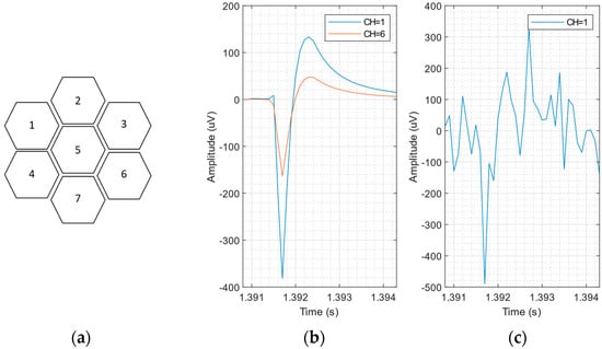
Figure 1.
(a) The 7-honeycomb sensor pattern (b) signals detected by pixel #1 and pixel #6, for a neuron positioned on the west side of the sensor (in the absence of interference and noise). (c) Synthetic neural recording with SNR = 3 dB, adding white noise on a noiseless synthetic recording.
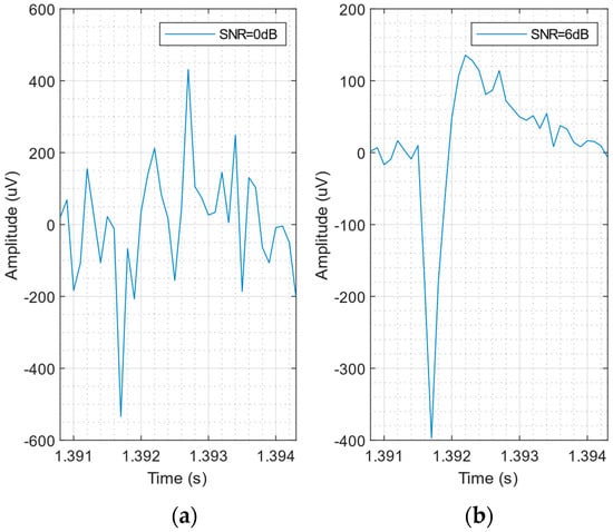
Figure 2.
Signal detected by pixel #1 for a neuron positioned on the west side of the sensor at different SNR levels, adding white noise on a noiseless synthetic recording. (a) SNR = 0 dB and (b) SNR = 6 dB.
In the spike detection pipeline the synthetic signal is firstly filtered with a 4th-order passband Butterworth filter (300–3000 Hz) to eliminate low-frequency LFP and to limit high-frequency thermal noise before further processing []. Therefore, to reduce CPU time, we keep the generation of the synthetic data simple and fast, considering only the thermal noise superimposed to the noiseless simulated extracellular recording.
2.3. SNEO Algorithm
Energy operators basically measure the cross energy between a signal and its derivatives []. A spike may be described as a short-lived burst with high amplitude and frequency; therefore, this class of operators enhances the differentiation between spikes and noise, improving the signal-to-noise ratio (SNR). This property and the low hardware complexity make the spike detection algorithm based on an energy operator suitable for on-chip implementation [,]. A popular technique is the non-linear energy operator (NEO), sometimes known as teager energy operator (TEO) []. In discrete time, the NEO φ of a signal x(n) is defined as:
Equation (4) describes how the NEO emphasizes both localized high energy and frequency on input signal: it is large only when the signal is high in power (i.e., large magnitude) and changing fast (i.e., high frequency) [].
The multi-resolution version of NEO (k-NEO) [] is introduced to improve detection performance at a low SNR. The k-NEO operator introduces a resolution parameter k and is described as follows:
The k-NEO output is often smoothed by a window such as Bartlett or Hamming [], which is called Smoothed NEO, or SNEO, as described in Equation (6).
In the following we use the Hamming window of length 4k + 1, as suggested in []. Figure 3 shows how the value of k (and hence the window width) affects the SNEO output. In the following we used k = 4 as the best compromise between spike amplification and time resolution.
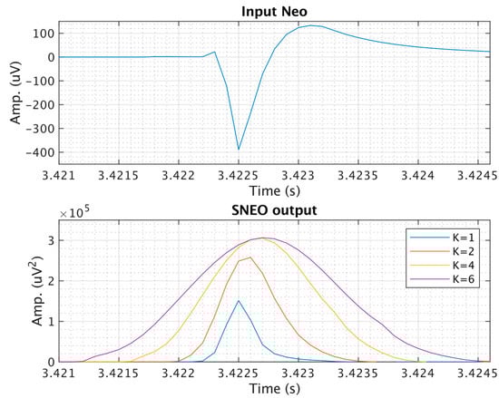
Figure 3.
The smoothed non-linear energy operator (SNEO) output at different resolution parameters considering a noiseless spike as input.
2.4. Thresholding
The threshold in any spike detection algorithm should be selected to maximize the probability of detecting the spikes, while keeping the number of false detections below a reasonable limit. The standard approach for SNEO is to take the threshold as a scaled version of the mean of :
where NC is the size of the sliding window used to estimate the mean, and C is the scale factor determined by the experiment with the ROC curves, as suggested in []. A schematic of the classical SNEO method is shown in Figure 4. Taking advantage of spatial correlation leads to a higher probability of detecting a true spike and thus improves performance. This is shown by the ROC curves in Figure 5.
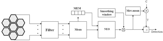
Figure 4.
SNEO block diagram. Signals from the seven channels are filtered and averaged, to exploit the correlation between data captured by adjacent pixels. The memory block (MEM) stores the samples needed to compute the nonlinear energy operator (NEO). Then, threshold T is a scaled version of the mean of the filtered NEO.
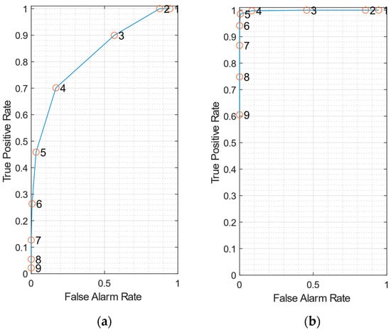
Figure 5.
(a) receiver operating characteristic (ROC) curve using data from a single pixel of the multi transistor arrays (MTA), for SNR = 3 dB. (b) ROC curve exploiting the correlation between signals coming from the 7 honeycomb pixels is exploited, for SNR = 3 dB. In both plots, true-positive and false-alarm rates are averaged on 10 datasets.
Figure 5a displays the ROC when data sampled from a single MTA pixel is employed for spike detection. By reducing the scale factor C, both true-positive rate and false-alarm rates increase, as expected. A FAR lower than 0.02 is obtained for C = 6, with a corresponding TPR of about 0.26.
Figure 5b shows the ROC obtained when the input of the k-NEO is obtained as the average of the signals coming from the 7 pixels of the sensor, to exploit the spatial correlation. The ROC curve increases much more steeply in this case. For C = 5, a FAR lower than 0.01 is obtained with a TPR of about 0.98. This example clearly shows that detection performance largely benefits from the correlation of the signals detected by the MTA pixels.
In the following analysis we consider simulated data for SNR = 0 dB. An example of the ROC curve at SNR = 0 dB and a sliding window of Nc = 5000 samples is shown in Figure 6a. The ROC shows that using C = 5 is a reasonable choice, giving a false-alarm rate of less than 0.02 (2%) and a respectable 60% accuracy even at SNR = 0 dB.
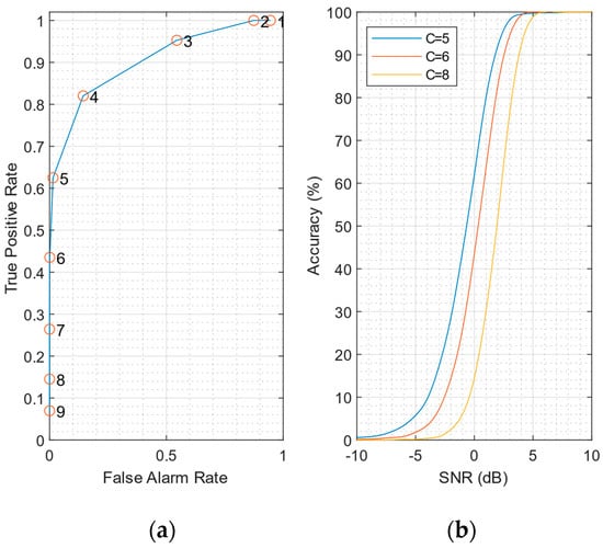
Figure 6.
(a) ROC curve at SNR = 0 dB, using the mean of the signals coming from the 7 honeycomb pixels. True-positive and false-alarm rates are averaged on 10 datasets. The scale factor C varies from 1 to 9. (b) Accuracy curves for different values of scale factor C.
Unfortunately, computing the threshold from the mean value of the SNEO operator results in performance degradation for high neuron firing rates. Figure 7 shows the accuracy curves for different neuron firing rates. As can be clearly observed, as the firing rate increases the detection performance worsens due to the increment of the threshold value. The accuracy at 0 dB SNR decreases from 60% for a firing rate of 10 Hz to about 25% when the firing rate reaches 200 Hz.
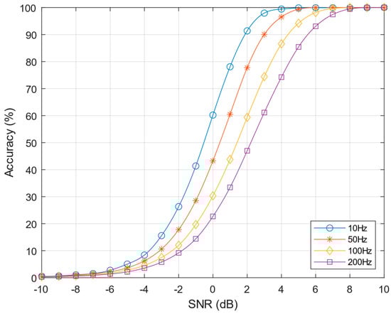
Figure 7.
SNEO accuracy at k = 4 varying the action potentials (APs) firing rate from 10–200 Hz, scale factor C = 5.
2.5. Proposed Approaches
To reduce the performance degradation for high firing rates, we have investigated two alternatives to the basic SNEO algorithm. Let us assume, for the time being, that the noise standard deviation σ is known beforehand (in practice, the σ value is estimated from the recorded neural signal—we will discuss some simple robust estimation techniques in Section 2.6).
In a first approach (that we name the following pre-normalization technique, or pre-norm) the signal coming from each channel, xi, is normalized (divided by) the corresponding channel noise standard deviation σi. Then, the mean of the normalized channel is calculated:
The SNEO operator is applied to x(n), and the result is compared with the threshold C. Figure 8 shows this implementation.
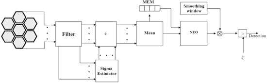
Figure 8.
Block diagram of the pre-norm technique. Each channel is normalized with its noise standard deviation estimate and then averaged and processed by SNEO. The comparison with the threshold C gives the detection result.
Figure 9 shows the improvement given by the pre-norm technique. The accuracy curves get closer to each other, showing the almost independence of the method from the neurons firing rates. The accuracy value at SNR = 0 dB is quite the same for the four firing rates (about 61%).
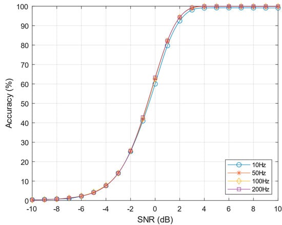
Figure 9.
Performances of pre-norm algorithm varying the neuron firing rate from 10–200 Hz, k = 4 and C = 7.
Unfortunately, the pre-norm technique requires a division to be performed for each channel. This increases the computational cost and makes this approach less amenable to hardware implementation.
To alleviate this problem, we developed a second algorithm named in the following post-normalization technique, or post-norm. In this algorithm, the mean of the signals coming from each channel is computed as:
xmean is sent to the SNEO operator, as in the basic algorithm of Section 2.4. The noise variance of xmean is estimated and a spike is detected when:
The post-norm algorithm avoids divisions and is depicted in the block diagram in Figure 10. As shown in Figure 11, the accuracy curves remain better and closer than the standard SNEO, with a slight performance decrease (about 1 dB) compared to the pre-norm approach.
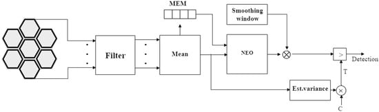
Figure 10.
Post-norm block diagram. The variance estimate block takes the averaged signal as input and estimates the noise variance.
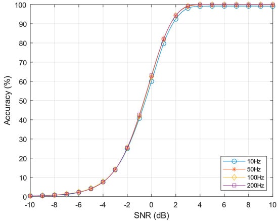
Figure 11.
Performance of post-norm algorithm varying the neurons firing rates from 10–200 Hz, k = 4 and C = 50.
2.6. Noise Estimation Techniques
Noise estimation techniques aim at estimating the noise distribution’s standard deviation σ, starting from recorded data that include spikes. Spikes are outliers with respect to background noise and affect the signal distributions, leading to an overestimation of σ [].
Please note that in the following discussion we assume that the signal x has zero mean thanks to the 2nd-order high pass filtering.
2.6.1. Median
The most well-known robust statistical method to estimate the background noise is based on computing the median of absolute value of the signal, scaled by a numerical factor of 0.6745, assuming a Gaussian noise distribution as in []:
where x(n) is the sample of the waveform at time n. This technique will be named median absolute deviation (MAD) in the following. Please note that the median requires us to sort a large array of neural samples, which requires a lot of computational resources and precludes a low-power hardware implementation [].
2.6.2. Mean Absolute
A simpler way to estimate the background noise is simply to take the root mean square of x(n), but the main issue of this straightforward technique is its dependency from the spike firing rates, which degrades the overall performance of the spike detection []. A viable alternative is using the absolute value of the signal in the moving average. This limits the error in the estimate due to spikes, since spike amplification by the squaring is avoided, while keeping low the complexity of the hardware implementation. The new σ estimation is defined as follows:
where M is the length of the moving average window, while the coefficient 1.25 is computed so that σn is equal to the standard deviation of x, when x is a zero-mean signal with a Gaussian distribution. Considering the main operations required for this estimate, we name this technique absolute average, or AA.
2.6.3. Winsorization
Another, more robust approach we propose is based on a technique called winsorization. The idea is to truncate the high value samples in the signal that come, with high probability, from spike outliers. In this way the clipped signal is mainly composed of noise, and we can obtain a robust estimate of σ from it [] (a similar technique is the kappa-sigma clipping used in astronomy []). Our implementation of winsorization method follows three steps:
- An initial noise standard deviation σ′ is required for the clipping (we used AA for this initial estimate).
- σ′ is then used for the clipping of the absolute value of the signal as follows:
- from the clipped signal x′(n), the standard deviation is finally estimated as:where the coefficient 1.58 is computed so that is equal to the standard deviation of x, when x is a zero-mean signal with a Gaussian distribution.
Since this approach combines winsorization and a moving average operation, we name this technique winsorization average, or WA, in the following.
3. Results
3.1. Performance Results
The values reported in the following have been obtained by averaging the results of 10 independent simulations, for each firing rate and SNR value. In all cases, the scale factor C has been chosen to obtain an accuracy not lower than 60% for a 10 Hz firing rate and a FAR lower than 0.02 at SNR = 0 dB. The detection performances for the standard SNEO and the proposed approaches at SNR = 0 dB for each firing rate are summarized in Table 1, Table 2 and Table 3, respectively.

Table 1.
Detection performances of Standard SNEO at different firing rates at SNR = 0 dB (C = 5).
Table 2.
Detection performances of pre-norm algorithm at different firing rates at SNR = 0 dB (C = 7).
Table 3.
Detection performances of post-norm algorithm at different firing rates at SNR = 0 dB (C = 50).
Figure 12 compares the performance of the investigated noise estimation techniques applied to the pre-norm algorithm, using the scale factor of 10 Hz (C = 7). As can be observed, the three sigma estimation techniques perform equally well in this case, with results very close to the ones in Figure 9 (that assumes an a-priori knowledge of the sigma). As a result, the simple AA approach is preferred, due to its simplicity.
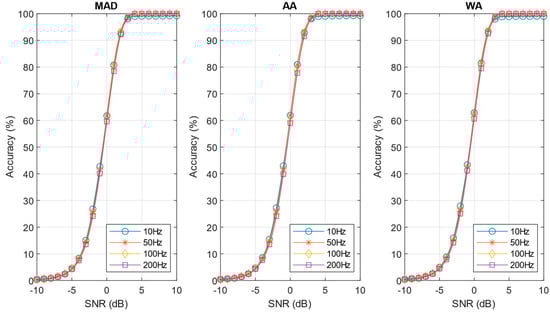
Figure 12.
Performances of pre-norm algorithm with the investigated noise estimation techniques. The neuron firing rate varies 10–200 Hz (C = 7).
The accuracy curves for the post-norm algorithm are shown in Figure 13. In this case the sigma estimation technique plays an important role in defining accuracy, and the results are less optimistic than shown in Figure 11. The detection decrease is also evident comparing the performance values of the pre-norm and post-norm approach reported in Table 2 and Table 3, respectively. It can be observed from Figure 13 that the WA estimate give remarkably good results, very close to the MAD technique, while being much simpler and more amenable to hardware implementation. The simpler AA estimate, while giving better results compared to the standard SNEO algorithm, is less effective that WA (see Table 3).
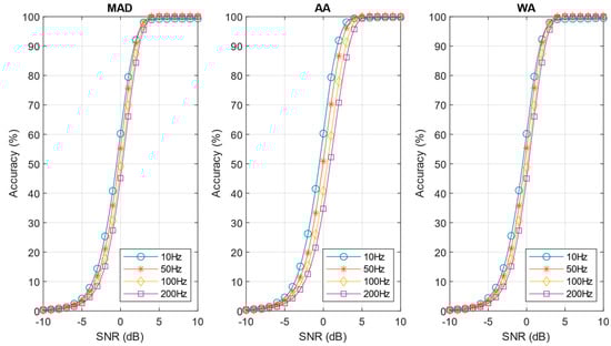
Figure 13.
Performances of post-norm algorithm with the investigated noise estimation techniques (C = 50).
3.2. Resource Consumption
The hardware complexity of the investigated algorithms can be estimated by considering the required arithmetic operations and their hardware cost, in terms of logic gates.
The cost of each arithmetic operator is assumed as: adder 5N, multiplier 6N2, division 13N + 20N2, comparator 7N, and register 9N, where N is the number of bits.
Table 4 reports the complexity estimate of the blocks in common between the investigated techniques (input filter, the mean of the seven channels, and SNEO), while the resources needed for the noise estimates AA and WA are listed in Table 5. We have not considered the MAD technique that requires the sorting of an array of values and is not suited for hardware implementation []. The additional computational resources required to implement each detector are shown in Table 6.
Table 4.
Resources required by the hardware implementation of common blocks. The division by 7 in the mean block is implemented by a multiplication for the inverse of 7.
Table 5.
Resources required by the hardware implementation of noise estimate blocks. The length M of the window is assumed to be a power of 2, to avoid hardware division.
Table 6.
Additional resources to build up each detector.
4. Discussion
Figure 14 shows the accuracy curves averaged on the four firing rates considered (10 Hz, 50 Hz, 100 Hz, 200 Hz); Figure 14a refers to the pre-norm approach, and Figure 14b to the post-norm approach. Table 7 summarizes the averaged detection performances at SNR = 0 dB and the hardware complexity. The number of logic gates has been estimated considering the SNEO tuning parameter k = 4 and assuming values encoded on N = 8-bit number, which is a typical value for power-constrained applications [,].
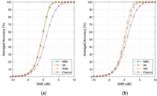
Figure 14.
Averaged accuracy curves. (a) pre-norm and Classic SNEO; (b) post-norm and Classic SNEO.
Table 7.
Averaged detection performance at SNR = 0 dB and computational cost (N = 8, k = 4).
The results in Figure 14a and in Table 7 show that the accuracy of the pre-norm approach outperforms the classic SNEO by a factor of 1.5× at 0 dB SNR. The false-alarm rate is larger that SNEO but still has an acceptable value, lower than 0.6%. The estimated number of logic gates for the pre-norm algorithm, however, is more than 1.2× compared to the standard SNEO method (mainly for the need of hardware divider), making this technique less attractive when low power is the main concern.
The post-norm approach shows a decrease of performance compared to pre-norm, and the choice of noise estimate method, moreover, influences the detection results. The MAD and WA estimates provides almost the same performance, while AA sigma estimates result in a 7% accuracy reduction (see Table 7). In any case, post-norm gives a better detection performance than classic SNEO in terms of accuracy and sensitivity (TPR). The MAD/WA accuracy outperforms classic SNEO by a factor of 1.3× at 0 dB SNR, while the AA outperforms SNEO by a factor of 1.1×, as summarized in Table 7. The false-alarm rate is larger that SNEO but remains below 0.5%. The post-norm technique is ideally suited for hardware implementation, not requiring any division. This is clearly shown in Table 7: the post-norm WA requires only 6% more logic gates compared to standard SNEO, while post-norm AA requires only 4% more gates.
5. Conclusions
In this paper we have investigated the performance achievable by using spike detection algorithms for CMOS multi transistors arrays, based on some variants of smoothed non-linear energy operator. We have shown that detection performance benefits from the correlation of the signals detected by the MTA pixels, but degrades when a high firing rate of neurons occurs. To solve this problem, we have presented two algorithm variants (pre-norm and post-norm) and two noise estimation techniques. In addition, a first order estimate of the number of logic gates required for hardware implementation of the investigated peak detection algorithms has been presented, to find the most suitable technique for an implantable on-chip implementation.
The pre-norm method shows an overall increase of 30% with respect to standard SNEO in terms of accuracy and sensitivity even when the simple AA noise estimation technique is employed. Unfortunately, the use of dividers makes this algorithm less amenable to hardware implementation. Hence, pre-norm can be useful when spike detection is not performed in the sensors themselves and adequate computational resources are available. The post-norm technique, while not as accurate as the pre-norm one, provides an accuracy and sensitivity improvement of 22% compared to the classic SNEO, with a reduced dependence on the neuronal firing rate. For post-norm, the WA noise estimation technique is a good choice, being simple to implement and similar in performance with the median absolute deviation estimate. This makes post-norm with WA noise estimate a suitable candidate for implantable MTA spike detectors.
On the basis of the obtained results, further investigation will be devoted to the VLSI implementation of post-norm algorithms.
Author Contributions
Conceptualization: G.S. and A.G.M.S.; methodology: G.S., M.T., E.A.V., and S.V.; software: G.S. and M.T.; writing—original draft preparation: G.S.; writing—review: G.S. and A.G.M.S.; supervision: S.V., A.G.M.S., A.B., and M.D.M.; funding acquisition, S.V., A.G.M.S., A.B. and M.D.M. All authors have read and agreed to the published version of the manuscript.
Funding
This research was supported by the Brain28 nm PRIN project, founded by MIUR.
Data Availability Statement
The data presented in this study are available on request from the first author.
Conflicts of Interest
The authors declare no conflict of interest.
References
- Berényi, A.; Somogyvári, Z.; Nagy, A.J.; Roux, L.; Long, J.D.; Fujisawa, S.; Stark, E.; Leonardo, A.; Harris, T.D.; Buzsáki, G. Large-Scale, High-Density (up to 512 Channels) Recording of Local Circuits in Behaving Animals. J. Neurophysiol. 2014, 111, 1132–1149. [Google Scholar] [CrossRef] [PubMed]
- Zhu, Q.; Cai, Y.; Fang, L.; Liang, X.; Ye, X.; Liang, B. A Lithops-Like Pt Nanorods Modified Microelectrode Array for Cellular ATP Release Detection. In Proceedings of the 2018 IEEE SENSORS, New Delhi, India, 28–31 October 2018; pp. 1–3. [Google Scholar]
- Tambaro, M.; Vallicelli, E.A.; Saggese, G.; Strollo, A.; Baschirotto, A.; Vassanelli, S. Evaluation of In Vivo Spike Detection Algorithms for Implantable MTA Brain—Silicon Interfaces. J. Low Power Electron. Appl. 2020, 10, 26. [Google Scholar] [CrossRef]
- Vallicelli, E.A.; Fary, F.; Baschirotto, A.; de Matteis, M.; Reato, M.; Maschietto, M.; Rocchi, F.; Vassanelli, S.; Guarrera, D.; Collazuol, G.; et al. Real-Time Digital Implementation of a Principal Component Analysis Algorithm for Neurons Spike Detection. In Proceedings of the 2018 International Conference on IC Design & Technology (ICICDT), Otranto, Italy, 4–6 June 2018; pp. 33–36. [Google Scholar]
- Vallicelli, E.A.; De Matteis, M.; Baschirotto, A.; Rescati, M.; Reato, M.; Maschietto, M.; Vassanelli, S.; Guarrera, D.; Collazuol, G.; Zeiter, R. Neural Spikes Digital Detector/Sorting on FPGA. In Proceedings of the 2017 IEEE Biomedical Circuits and Systems Conference (BioCAS), Turin, Italy, 19–21 October 2017; pp. 1–4. [Google Scholar]
- Tambaro, M.; Vallicelli, E.A.; Tomasella, D.; Baschirotto, A.; Vassanelli, S.; Maschietto, M.; De Matteis, M. Real-Time Neural (RT-Neu) Spikes Imaging by a 9375 Sample/(Sec Pixel) 32×32 Pixels Electrolyte-Oxide-Semiconductor Biosensor. In Proceedings of the 2019 15th Conference on Ph.D Research in Microelectronics and Electronics (PRIME), Lausanne, Switzerland, 15–18 July 2019; pp. 233–236. [Google Scholar]
- Miccoli, B.; Lopez, C.M.; Goikoetxea, E.; Putzeys, J.; Sekeri, M.; Krylychkina, O.; Chang, S.-W.; Firrincieli, A.; Andrei, A.; Reumers, V.; et al. High-Density Electrical Recording and Impedance Imaging With a Multi-Modal CMOS Multi-Electrode Array Chip. Front. Neurosci. 2019, 13, 641. [Google Scholar] [CrossRef] [PubMed]
- Obeid, I.; Wolf, P.D. Evaluation of Spike-Detection Algorithms for a Brain-Machine Interface Application. IEEE Trans. Biomed. Eng. 2004, 51, 905–911. [Google Scholar] [CrossRef] [PubMed]
- Do, A.T.; Yeo, K.S. A Hybrid NEO-Based Spike Detection Algorithm for Implantable Brain-IC Interface Applications. In Proceedings of the 2014 IEEE International Symposium on Circuits and Systems (ISCAS), Melbourne VIC, Australia, 1–5 June 2014; pp. 2393–2396. [Google Scholar]
- Thies, J.; Alimohammad, A. Compact and Low-Power Neural Spike Compression Using Undercomplete Autoencoders. IEEE Trans. Neural Syst. Rehabil. Eng. 2019, 27, 1529–1538. [Google Scholar] [CrossRef] [PubMed]
- Tariq, T.; Satti, M.H.; Saeed, M.; Kamboh, A.M. Low SNR Neural Spike Detection Using Scaled Energy Operators for Implantable Brain Circuits. In Proceedings of the 2017 39th Annual International Conference of the IEEE Engineering in Medicine and Biology Society (EMBC), Jeju, Korea, 11–15 July 2017; pp. 1074–1077. [Google Scholar]
- Eisen, E.S.; Toreyin, H. A Preliminary Analysis on Impact of Additive Flicker Noise on Detection Sensitivity of Neural Spikes. In Proceedings of the 2019 41st Annual International Conference of the IEEE Engineering in Medicine and Biology Society (EMBC), Berlin, Germany, 23–27 July 2019; pp. 5164–5167. [Google Scholar]
- Mirzaei, S.; Hosseini-Nejad, H.; Sodagar, A.M. Spike Detection Technique Based on Spike Augmentation with Low Computational and Hardware Complexity. In Proceedings of the 2020 42nd Annual International Conference of the IEEE Engineering in Medicine & Biology Society (EMBC), Montreal, QC, Canada, 20–24 July 2020; pp. 894–897. [Google Scholar]
- Huang, L.; Ling, B.W.-K.; Cai, R.; Zeng, Y.; He, J.; Chen, Y. WMsorting: Wavelet Packets’ Decomposition and Mutual Information-Based Spike Sorting Method. IEEE Trans. Nanobiosci. 2019, 18, 283–295. [Google Scholar] [CrossRef] [PubMed]
- Schaffer, L.; Nagy, Z.; Kineses, Z.; Fiath, R. FPGA-Based Neural Probe Positioning to Improve Spike Sorting with OSort Algorithm. In Proceedings of the 2017 IEEE International Symposium on Circuits and Systems (ISCAS), Baltimore, MD, USA, 28–31 May 2017; pp. 1–4. [Google Scholar]
- Barzan, H.; Ichim, A.-M.; Muresan, R.C. Machine Learning-Assisted Detection of Action Potentials in Extracellular Multi-Unit Recordings. In Proceedings of the 2020 IEEE International Conference on Automation, Quality and Testing, Robotics (AQTR), Cluj-Napoca, Romania, 21–23 May 2020; pp. 1–5. [Google Scholar]
- Shaikh, S.; So, R.; Libedinsky, C.; Basu, A. Experimental Comparison of Hardware-Amenable Spike Detection Algorithms for IBMIs. In Proceedings of the 2019 9th International IEEE/EMBS Conference on Neural Engineering (NER), San Francisco, CA, USA, 20–23 March 2019; pp. 754–757. [Google Scholar]
- Sablok, S.; Gururaj, G.; Shaikh, N.; Shiksha, I.; Choudhary, A.R. Interictal Spike Detection in EEG Using Time Series Classification. In Proceedings of the 2020 4th International Conference on Intelligent Computing and Control Systems (ICICCS), Madurai, India, 13–15 May 2020; pp. 644–647. [Google Scholar]
- Abd El-Samie, F.E.; Alotaiby, T.N.; Khalid, M.I.; Alshebeili, S.A.; Aldosari, S.A. A Review of EEG and MEG Epileptic Spike Detection Algorithms. IEEE Access 2018, 6, 60673–60688. [Google Scholar] [CrossRef]
- Brychta, R.J.; Shiavi, R.; Robertson, D.; Diedrich, A. Spike Detection in Human Muscle Sympathetic Nerve Activity Using the Kurtosis of Stationary Wavelet Transform Coefficients. J. Neurosci. Methods 2007, 160, 359–367. [Google Scholar] [CrossRef] [PubMed]
- Beche, J.-F.; Bonnet, S.; Levi, T.; Escola, R.; Noca, A.; Charvet, G.; Guillemaud, R. Real-Time Adaptive Discrimination Threshold Estimation for Embedded Neural Signals Detection. In Proceedings of the 2009 4th International IEEE/EMBS Conference on Neural Engineering, Antalya, Turkey, 29 April–2 May 2009; pp. 597–600. [Google Scholar]
- Pregowska, A.; Kaplan, E.; Szczepanski, J. How Far Can Neural Correlations Reduce Uncertainty? Comparison of Information Transmission Rates for Markov and Bernoulli Processes. Int. J. Neur. Syst. 2019, 29, 1950003. [Google Scholar] [CrossRef] [PubMed]
- Pregowska, A.; Casti, A.; Kaplan, E.; Wajnryb, E.; Szczepanski, J. Information Processing in the LGN: A Comparison of Neural Codes and Cell Types. Biol. Cybern. 2019, 113, 453–464. [Google Scholar] [CrossRef] [PubMed]
- Camuñas-Mesa, L.A.; Quiroga, R.Q. A Detailed and Fast Model of Extracellular Recordings. Neural Comput. 2013, 25, 1191–1212. [Google Scholar] [CrossRef] [PubMed]
- Gibson, S.; Judy, J.W.; Markovic, D. Technology-Aware Algorithm Design for Neural Spike Detection, Feature Extraction, and Dimensionality Reduction. IEEE Trans. Neural Syst. Rehabil. Eng. 2010, 18, 469–478. [Google Scholar] [CrossRef] [PubMed]
- Mondragón-González, S.L.; Burguière, E. Bio-Inspired Benchmark Generator for Extracellular Multi-Unit Recordings. Sci. Rep. 2017, 7, 43253. [Google Scholar] [CrossRef] [PubMed]
- Ng, A.K.; Ang, K.K.; Guan, C. Automatic Selection of Neuronal Spike Detection Threshold via Smoothed Teager Energy Histogram. In Proceedings of the 2013 6th International IEEE/EMBS Conference on Neural Engineering (NER), San Diego, CA, USA, 6–8 November 2013; pp. 1437–1440. [Google Scholar]
- Yang, Y.; Mason, A.J. Hardware Efficient Automatic Thresholding for NEO-Based Neural Spike Detection. IEEE Trans. Biomed. Eng. 2017, 64, 826–833. [Google Scholar] [CrossRef] [PubMed]
- Do, A.T.; Zeinolabedin, S.M.A.; Jeon, D.; Sylvester, D.; Kim, T.T.-H. An Area-Efficient 128-Channel Spike Sorting Processor for Real-Time Neural Recording With 0.175 μW/Channel in 65-Nm CMOS. IEEE Trans. VLSI Syst. 2019, 27, 126–137. [Google Scholar] [CrossRef]
- Osipov, D.; Paul, S.; Stemmann, H.; Kreiter, A.K. Energy-Efficient Architecture for Neural Spikes Acquisition. In Proceedings of the 2018 IEEE Biomedical Circuits and Systems Conference (BioCAS), Cleveland, OH, USA, 17–19 October 2018; pp. 1–4. [Google Scholar]
- Schaffer, L.; Pletl, S.; Kincses, Z. Spike Detection Using Cross-Correlation Based Method. In Proceedings of the 2019 IEEE 23rd International Conference on Intelligent Engineering Systems (INES), Gödöllő, Hungary, 25–27 April 2019; pp. 000175–000178. [Google Scholar]
- Choi, J.H.; Jung, H.K.; Kim, T. A New Action Potential Detector Using the MTEO and Its Effects on Spike Sorting Systems at Low Signal-to-Noise Ratios. IEEE Trans. Biomed. Eng. 2006, 53, 738–746. [Google Scholar] [CrossRef] [PubMed]
- Gibson, S.; Judy, J.W.; Markovic, D. Comparison of Spike-Sorting Algorithms for Future Hardware Implementation. In Proceedings of the 2008 30th Annual International Conference of the IEEE Engineering in Medicine and Biology Society, Vancouver, BC, Canada, 20–25 August 2008; pp. 5015–5020. [Google Scholar]
- Quiroga, R.Q.; Nadasdy, Z.; Ben-Shaul, Y. Unsupervised Spike Detection and Sorting with Wavelets and Superparamagnetic Clustering. Neural Comput. 2004, 16, 1661–1687. [Google Scholar] [CrossRef] [PubMed]
- Rizk, M.; Wolf, P.D. Optimizing the Automatic Selection of Spike Detection Thresholds Using a Multiple of the Noise Level. Med. Biol. Eng. Comput. 2009, 47, 955–966. [Google Scholar] [CrossRef] [PubMed]
- Pastor, D.; Socheleau, F.-X. Robust Estimation of Noise Standard Deviation in Presence of Signals With Unknown Distributions and Occurrences. IEEE Trans. Signal Process. 2012, 60, 1545–1555. [Google Scholar] [CrossRef]
- Sánchez-Monge, Á.; Schilke, P.; Ginsburg, A.; Cesaroni, R.; Schmiedeke, A. STATCONT: A Statistical Continuum Level Determination Method for Line-Rich Sources. Astron. Astrophys. 2018, 609, A101. [Google Scholar] [CrossRef]
- Tai, M.-Y.; Tu, W.-C.; Chien, S.-Y. VLSI Architecture Design of Layer-Based Bilateral and Median Filtering for 4k2k Videos at 30 fps. In Proceedings of the 2017 IEEE International Symposium on Circuits and Systems (ISCAS), Baltimore, MD, USA, 28–31 May 2017; pp. 1–4. [Google Scholar]
Publisher’s Note: MDPI stays neutral with regard to jurisdictional claims in published maps and institutional affiliations. |
© 2021 by the authors. Licensee MDPI, Basel, Switzerland. This article is an open access article distributed under the terms and conditions of the Creative Commons Attribution (CC BY) license (http://creativecommons.org/licenses/by/4.0/).