Input-Series-Output-Parallel DC Transformer Impedance Modeling and Phase Reshaping for Rapid Stabilization of MVDC Distribution Systems

Abstract

This paper focuses on the instability problem of the medium-voltage DC (MVDC) distribution system and proposes an impedance phase reshaping (IPR) method. To obtain the load impedance model of the MVDC distribution system, the input impedance of the input-series-output-parallel (ISOP) DC transformer (DCT) is derived by the generalized average modeling (GAM). Based on the obtained model, the traditional ISOP DCT controller optimization (IDCO) approach is discussed and the IPR method is developed. An impedance phase controller is introduced based on the original control method. According to the optimized impedance stability criterion, the parameters of the impedance phase controller are determined. Compared with the IDCO approach, the proposed method weakens the negative resistance characteristic of the load impedance at the resonant frequency. Therefore, the MV bus voltage oscillation is rapidly mitigated. Besides, the dynamic performance of the system using the IPR method can be classified as good. The simulation results show that the mathematical model is correct, and the proposed method is effective for the rapid stabilization of MVDC distribution systems.

1. Introduction

The medium-voltage DC (MVDC) distribution system has become the trend of the future energy internet power distribution due to the beneficial attributes, such as its flexibility and efficiency [1,2,3]. An MVDC grid was designed for the interconnection of high-power test benches at a university campus [4]. Furthermore, the MVDC power distribution has been widely applied in railway electrification systems and marine electrical distribution systems [5,6,7,8,9,10].

A typical DC distribution system is shown in Figure 1. The DC transformer (DCT) plays a prominent role in the modern MVDC distribution system. As the key device, it connects the MVDC bus and the low-voltage DC (LVDC) bus. Given the voltage stress of the switching devices, the inputs-series-output-parallel (ISOP) topology of several DC/DC converter modules has been introduced. For the ISOP DCT, the dual-active bridge (DAB) converter is a more suitable submodule than other converters, such as the bidirectional half-bridge converter and the series resonant converter [11,12]. In addition, an input voltage sharing (IVS) control strategy has been presented to ensure the power sharing of the ISOP DCT [13,14]. However, a tightly regulated converter behaves as a constant power load (CPL) [15,16,17,18], which exhibits a negative resistance characteristic and may destabilize the system. When a regulated ISOP DCT is connected to a power electronic converter or an inductive circuit as shown in Figure 1, the stability of the MVDC distribution system may become corrupted and substantial oscillations would occur. Besides, it has been confirmed that the system behaves in an unstable way with the increase of the source-side inductance [19,20,21]. Consequently, an impedance-based stability analysis for the ISOP DCT is essential to guarantee the stability of the MVDC distribution system.

The prerequisite for the impedance-based stability analysis is to develop the impedance model of the system, including the source impedance and the load impedance. Based on the model, the stability of the system can be analyzed by the impedance stability criterion.

Several theoretical modeling techniques have been proposed to obtain an impedance model. Taking the first harmonic approximation into consideration, the generalized average modeling (GAM) [22,23,24] is more accurate than the reduced-order modeling [25] for the DAB converter. Based on the impedance model, Middlebrook et al. discussed the stability criterion for voltage regulated DC/DC converters [26], and Sun et al. studied the stability criterion for grid-connected inverters [27]. The ratio of the source impedance and the load impedance is known as the minor loop gain, and the whole system is stable if it satisfies the Nyquist Criterion [28]. Moreover, various stability criteria have been proposed by defining the constraint boundary of the minor loop gain [29,30]. Riccobono et al. [31] presented a Passivity-Based Stability Criterion (PBSC), which increases the phase of the system total impedance up to 0° at the resonant frequency. Hence, the impedance becomes passive to guarantee the bus stability [32,33].

According to the above-mentioned stability criteria, the system stability can be improved by reshaping the impedance. Feng et al. [34] introduced two control methods to modify the impedance by building a virtual impedance connected in parallel or series with the input impedance of the DAB converter. There was no intersection of the impedance amplitude by increasing the input impedance amplitude. In [35], a resonance term was applied to dampen the bus impedance. However, this approach only relies on the source impedance and ignores the influence of the load impedance. Compared with the impedance amplitude reshaping, the phase modification takes into account that the amplitude must intersect. Zhang et al. [36] proposed a parallel virtual impedance (PVI) and a series virtual impedance (SVI) control strategy to modify the load impedance phase at a small range of frequency. According to the approaches introduced in [36], Feng et al. [37] analyzed the stability improvement of the system via the controller optimization. Meanwhile, an impedance shaping regulator has been proposed to reshape the impedance phase. Although they both enhance the stability of the DAB-based energy storage systems, the impedance shaping regulator has better dynamic responses than the optimized method of the DAB controller. The system with the optimized DAB controller requires minimum cost. Moreover, Guan et al. [38] proposed a three-closed-loop control strategy to reshape the input impedance of the DAB converter. On the basis of the control method introduced in [38], Wang et al. [39] investigated a triple-close-loop IVS control strategy, which improved the dynamic and steady-state performance of the ISOP DCT. However, the strategy has drawbacks with complicated parameter calculation and extra design steps.

This paper proposes an impedance phase reshaping (IPR) method, the load impedance model is obtained by the GAM method, and the impedance phase is modified for the MVDC distribution system rapid stabilization.

This paper presents the following major contributions.

(1)

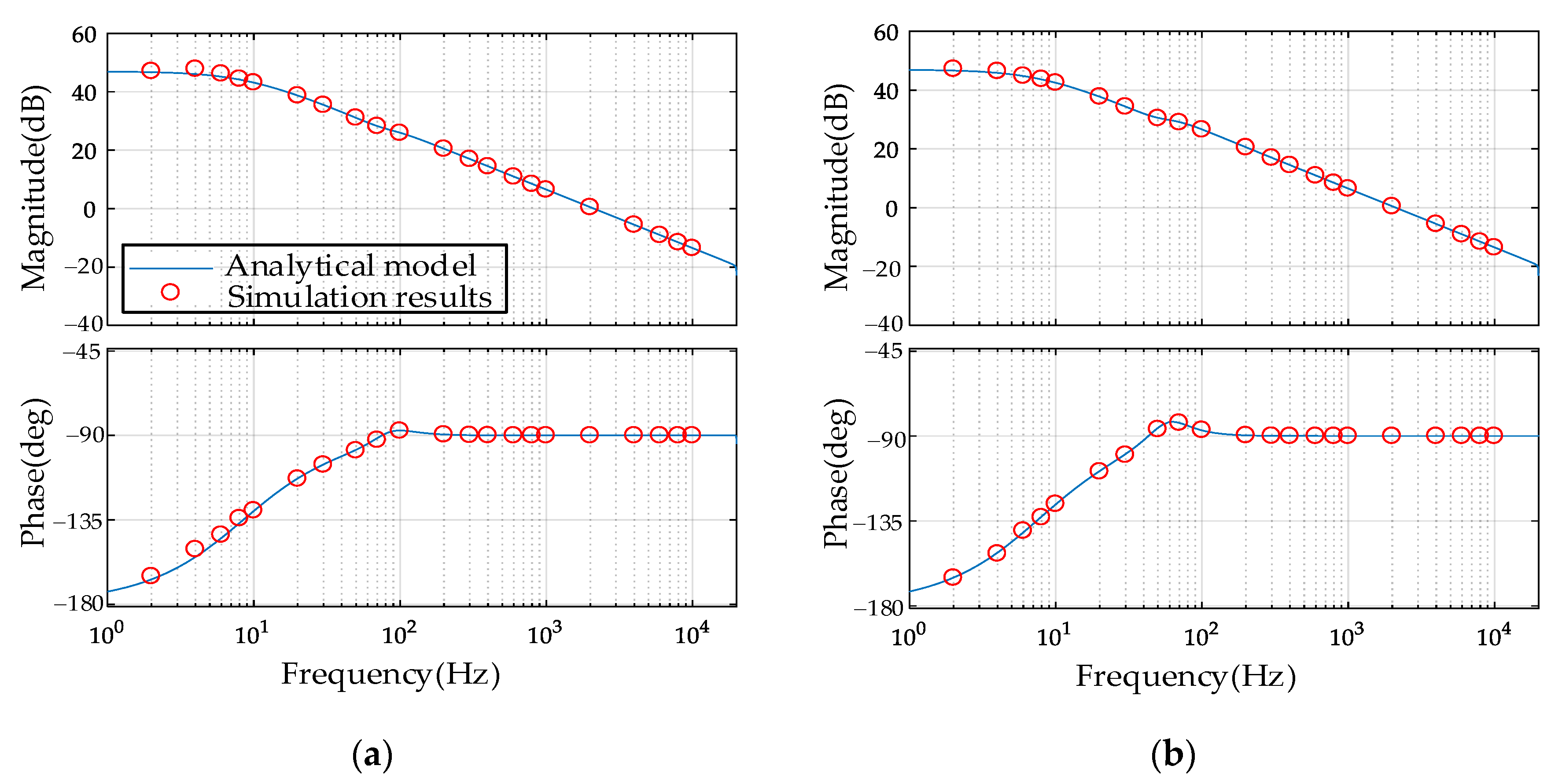
Establish a GAM input impedance model for the ISOP DCT. The obtained model is accurate and programmable, which provides a theoretical basis for the stability analysis.

(2)

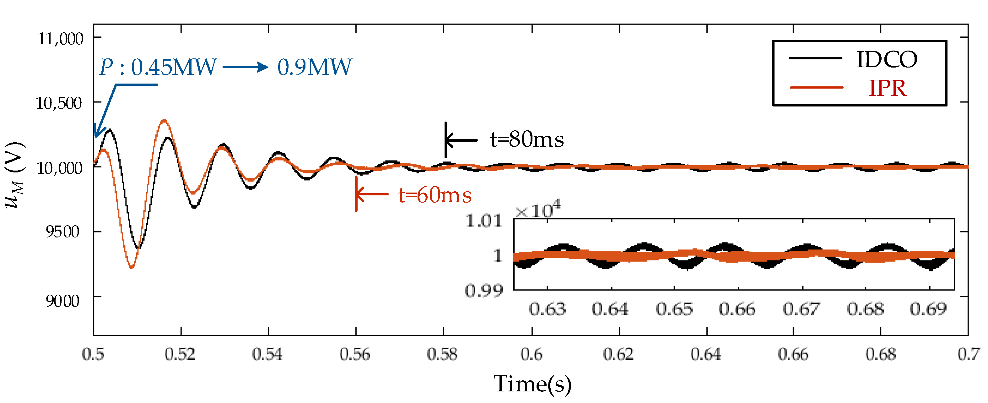
Propose an IPR method to modify the impedance phase, which weakens the negative resistance characteristic of the ISOP DCT. The ISOP DCT controller optimization (IDCO) method is investigated. Compared with the IDCO method, the proposed approach mitigates the MV bus voltage oscillation rapidly and improves the voltage quality of the ISOP DCT.

The paper is organized as follows. Section 2 introduces the configuration of the MVDC Distribution System, and the GAM input impedance model of the ISOP DCT is established as the load impedance. Section 3 describes the IDCO method. Section 4 discusses the proposed IPR method. Section 5 displays the simulation analysis results. Section 6 summarizes the major outcomes of this paper and its possible future extensions.

2. Impedance Modeling of the MVDC Distribution System

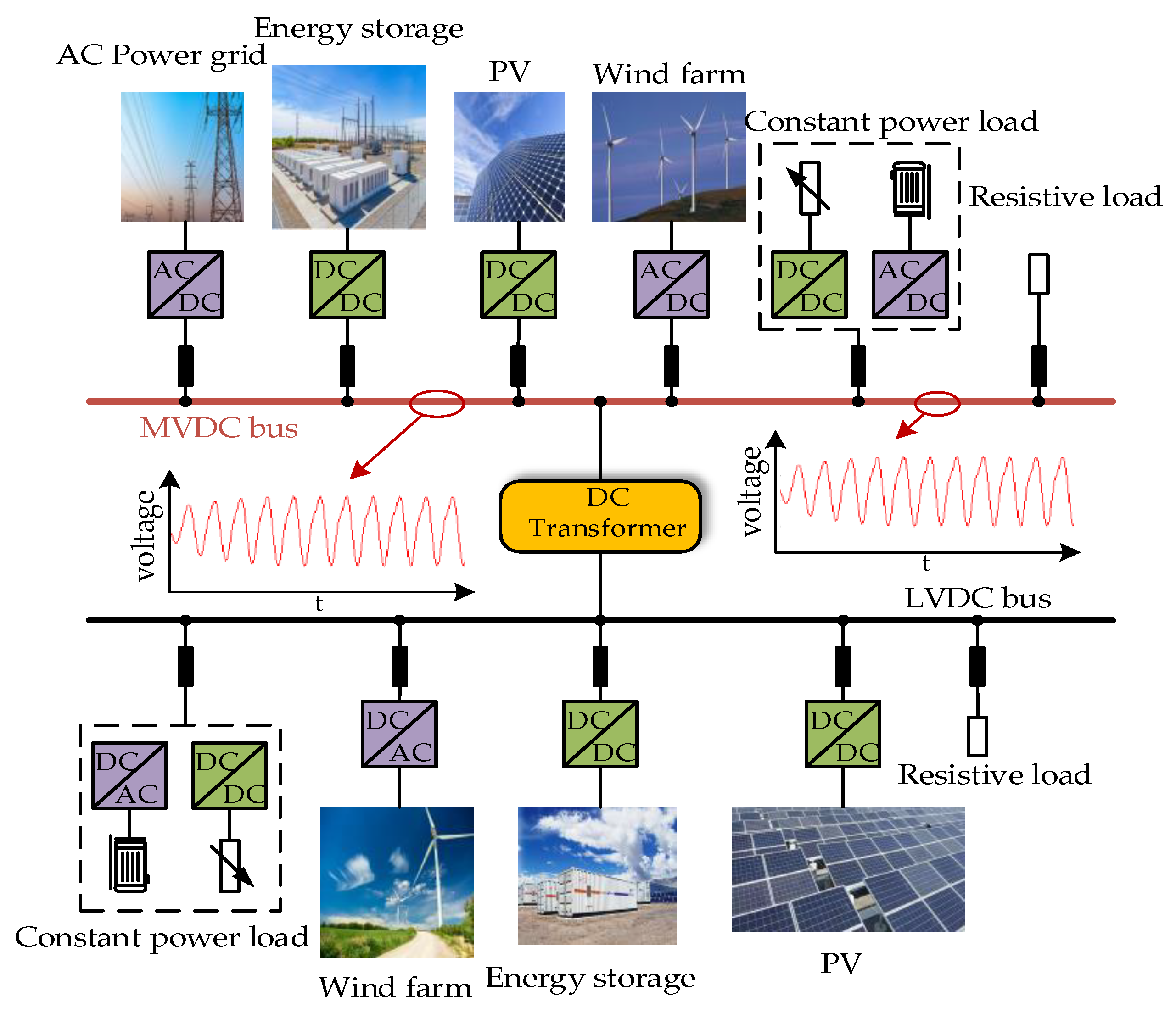
2.1. Configuration of the MVDC Distribution System

The MVDC distribution system includes the DC grid, the ISOP DCT, and the load. The structure of the MVDC distribution system is shown in Figure 2.

$R_L$ is the load impedance. $u_M$ and $u_L$ are the MVDC and the LVDC bus voltage, respectively. Meanwhile, $u_L$ is the voltage of the output capacitance $C_o$. In the DC grid, $V_g$ is the DC grid voltage, $L_g$ is the transmission line inductance. In the ISOP DCT, $C_o$ is the output capacitance, n (n ∈ N+, N+ is a set of positive integers) is the number of the DAB modules of the ISOP DCT. In the i-th (i = 1, 2 … n) DAB module, ${\mathrm{H}}_1$ and ${\mathrm{H}}_2$ are the rectifier and the inverter full bridges respectively. ${\mathrm{S}}_1\sim {\mathrm{S}}_8$ are the switches of the bridge arms. $i_L$ is the current of $L_s$. $C_{ini}$ is the input capacitance. K is the turns ratio of the high-frequency transformer. $L_s$ is the leakage inductance of the high-frequency transformer and resonant inductance. $u_{ini}$ and $i_p$ are the primary side voltage and current, respectively. Moreover, $u_M={\displaystyle {\sum }_{i=1}^n{u}_{ini}}$.

In addition, the control block diagram of the ISOP DCT is descripted in Figure 3. The input voltage sharing (IVS) control strategy of the ISOP DCT is illustrated in Figure 3. It consists of an output voltage controller $G_{u_L}$ and n − 1 input voltage sharing controllers $G_{u_M}$. $u_M^{*}$ and $u_L^{*}$ are the MV and the LV bus voltage, respectively. The commonly used single phase shift (SPS) method is adopted in this paper. $d_L$ is the basic phase shift ratio of each DAB module and is generated by the output voltage controller $G_{u_L}$. $d_{ini}$ (i = 1, 2 … n) is the compensation in phase shift ratio of the i-th DAB module, which is generated by the input voltage sharing controller $G_{u_M}$. $d_i$ (i = 1, 2 … n) is the phase shift ratio.

As can be seen from Figure 3, the phase shift ratio $d_i$ (i = 1, 2 … n) is the difference between the two items, which can be expressed as

$$d_i=d_L-d_{ini},$$

(1)

Moreover, the decoupling condition of the basic phase shift ratio $d_L$ and the compensation in phase shift ratio $d_{ini}$ (i = 1, 2 … n − 1) is defined as follows:

$$d_{inn}=-{\displaystyle \sum _{i=1}^{n-1}{d}_{ini}},$$

(2)

where $d_{inn}$ is the compensation in the phase shift ratio of the n-th DAB module.

Based on (2), the controllers of the ISOP DCT can be decoupled from each other. The phase shift ratio $d_i$ (i = 1, 2 … n) is a constant value when power sharing is achieved. Thus, assuming that the phase shift ratio $d_i=d$ (i = 1, 2 … n), then the load impedance modeling for the MVDC distribution system is as follows.

2.2. Generalized Average Modeling of the ISOP DCT

The load impedance model $Z_L(s)$ of the MVDC distribution system, i.e., the GAM input impedance model of the ISOP DCT is established in this section. The voltage $u_L$ of the output capacitance $C_o$ and the current $i_L$ of the inductance $L_s$ are selected as the state variables. Thus, the state equation of the ISOP DCT can be expressed as

$$\{\begin{array}{l}\frac{d{i}_L}{dt}=\frac{{\mathrm{s}}_1}{n{L}_s}{u}_M-\frac{K{\mathrm{s}}_2}{L_s}{u}_L,\\ \frac{d{u}_L}{dt}=\frac{Kn{\mathrm{s}}_2}{C_o}{i}_L-\frac{1}{C_o}\frac{u_L}{R_L},\end{array}$$

(3)

where ${\mathrm{s}}_1$ and ${\mathrm{s}}_2$ are the switching functions of the bridge ${\mathrm{H}}_1$ and ${\mathrm{H}}_2$ in the DAB converter, respectively.

Besides, the primary side current $i_p$ and the LV bus voltage $u_L$ are selected as the output variables. The output equation of the ISOP DCT can be given as

$$\{\begin{array}{l}{i}_p={\mathrm{s}}_1{i}_L,\\ u_L=u_L.\end{array}$$

(4)

Equations (3) and (4) are based heavily on the model in [22]. More detailed derivation of the state equation, output equation and switching functions ${\mathrm{s}}_1$ and ${\mathrm{s}}_2$ may be found therein.

Due to the pure alternating current characteristic of the inductor current $i_L$, the state-variable vector x is expressed as

$$\mathit{x}={\left[\begin{array}{ccc}<u_L{>}_0& <i_L{>}_{1\mathrm{R}}& <i_L{>}_{1\mathrm{I}}\end{array}\right]}^T,$$

(5)

where $<u_L{>}_0$ denotes the zeroth coefficient in the Fourier series of $u_L$. $<i_L{>}_{1\mathrm{R}}$ and $<i_L{>}_{1\mathrm{I}}$ denote the real part and imaginary part of the 1st coefficient in the Fourier series of $i_L$, respectively.

Similarly, the output vector y can be expressed as

$$\mathit{y}={\left[\begin{array}{cc}{i}_p& u^L\end{array}\right]}^T.$$

(6)

Substitute (5) into (3) and (4) and apply the small perturbation to d,$u_{ini}$ and the state variables at the steady-state operation point. After linearization, the small-signal matrix equation is given as

$$\{\begin{array}{l}\dot{\hat{\mathit{x}}}=\mathit{A}\hat{\mathit{x}}+\mathit{B}\hat{\mathit{u}},\\ \hat{\mathit{y}}=\mathit{C}\hat{\mathit{x}}+\mathit{D}\hat{\mathit{u}},\end{array}$$

(7)

where A, B, C and D are the constant matrixs. $u$ is the input vector. $\hat{\mathit{x}}$ and $\hat{\mathit{u}}$ represent the small signal value of the state-variable vector x and the input vector $\mathit{u}$, respectively. $\dot{\hat{\mathit{x}}}$ is the derivative of $\hat{\mathit{x}}$. $\hat{\mathit{y}}$ is the small signal value of the output vector y.

$$\hat{\mathit{x}}=\left[\begin{array}{l}<{\hat{u}}_L{>}_0\\ <{\hat{i}}_L{>}_{1\mathrm{R}}\\ <{\hat{i}}_L{>}_{1\mathrm{I}}\end{array}\right],$$

(8)

$$\hat{\mathit{y}}=\left[\begin{array}{l}{\hat{i}}_p\\ {\hat{u}}_L\end{array}\right],$$

(9)

$$\hat{\mathit{u}}=\left[\begin{array}{l}{\hat{u}}_{ini}\\ \hat{d}\end{array}\right],$$

(10)

$$\mathit{A}=\left[\begin{array}{ccc}\frac{-1}{R{C}_o}& \frac{-4Kn\sin (d\pi )}{\pi C_o}& \frac{-4Kn\cos (d\pi )}{\pi C_o}\\ \frac{2K\sin (d\pi )}{\pi L_s}& 0& {\omega }_s\\ \frac{2K\cos (d\pi )}{\pi L_s}& -{\omega }_s& 0\end{array}\right],$$

(11)

$$\mathit{B}=\left[\begin{array}{cc}0& -\frac{4Kn<i_L{>}_{1\mathrm{R}}\cos (d\pi )}{C_o}+\frac{4Kn<i_L{>}_{1\mathrm{I}}\sin (d\pi )}{C_o}\\ 0& \frac{2K<u_L{>}_0\cos (d\pi )}{L_s}\\ -\frac{2}{\pi L_s}& -\frac{2K<u_L{>}_0\sin (d\pi )}{L_s}\end{array}\right],$$

(12)

$$\mathit{C}=\left[\begin{array}{ccc}0& 0& -\frac{4}{\pi }\\ 1& 0& 0\end{array}\right],$$

(13)

$$\mathit{D}=\mathbf{0},$$

(14)

where ${\omega }_s=2\pi f_s$ and $f_s$ is the switching frequency of the ISOP DCT. $<{\hat{u}}_L{>}_0$, $<{\hat{i}}_L{>}_{1\mathrm{R}}$, $<{\hat{i}}_L{>}_{1\mathrm{I}}$, ${\hat{i}}_p$, ${\hat{u}}_L$, ${\hat{u}}_{ini}$ and $\hat{d}$ are the small signal values of $<u_L{>}_0$, $<i_L{>}_{1\mathrm{R}}$, $<i_L{>}_{1\mathrm{I}}$, $i_p$, $u_L$, $u_{ini}$ and d respectively.

Thus, combining (7)–(14), the open-loop transfer functions $Y_{op}(s)$, $G_{i_{p}d}(s)$, $G_{u_L{u}_{ini}}(s)$ and $G_{u_{L}d}(s)$ can be defined as

$$\left[\begin{array}{l}{\hat{i}}_p\\ {\hat{u}}_L\end{array}\right]=\left[\begin{array}{cc}{Y}_{op}(s)& G_{i_{p}d}(s)\\ G_{u_L{u}_{ini}}(s)& G_{u_{L}d}(s)\end{array}\right]\left[\begin{array}{l}{\hat{u}}_{ini}\\ \hat{d}\end{array}\right].$$

(15)

where $Y_{op}(s)$ is the transfer function from ${\hat{i}}_p$ to ${\hat{u}}_{ini}$, $G_{i_{p}d}(s)$ is the transfer function from ${\hat{i}}_p$ to $\hat{d}$, $G_{u_L{u}_{ini}}(s)$ is the transfer function from ${\hat{u}}_L$ to ${\hat{u}}_{ini}$ and $G_{u_{L}d}(s)$ is the transfer function from ${\hat{u}}_L$ to $\hat{d}$ respectively.

According to (15) and Figure 3, the small-signal block diagram of the i-th (i = 1, 2 … n − 1) DAB module is shown in Figure 4. ${\hat{u}}_L^{*}$ is the small-signal value of the LVDC bus reference voltage. ${\hat{u}}_{ini}^{*}$ is the small-signal value of the primary side reference voltage of the i-th (i = 1, 2 … n − 1) DAB module.

As can be seen from Figure 4, ${\hat{u}}_L^{*}$ and ${\hat{u}}_{ini}^{*}$ are zero. Given the input capacitance C_ini of the i-th (i = 1, 2 … n) DAB converter, the close-loop input admittance $Y_{L\_n-1}(s)$ for these n − 1 DAB modules is obtained as follows:

$$Y_{L\_n-1}(s)={\displaystyle \sum _{i=1}^{n-1}[Y_{op}(s)+Y_{ci}(s)-\frac{G_{u_L{u}_{ini}}(s)G_{u_L}(s)G_{i_{p}d}(s)}{1+G_{u_L}(s)G_{u_{L}d}(s)}+\frac{G_{u_M}(s)G_{i_{p}d}(s)}{1+G_{u_L}(s)G_{u_{L}d}(s)}]},$$

(16)

where Y_ci (s) is the admittance of the capacitance C_ini.

Similarly, the small-signal block diagram of the n-th DAB module is shown in Figure 5.

From Figure 5, we can see that the compensation in phase shift ratio $d_{inn}$ for the n-th DAB converter is different from $d_{ini}$ (i = 1, 2 … n − 1) for the i-th DAB converter as shown in Figure 4, which is caused by the decoupling condition expressed in (2). Based on the control block diagram, the close-loop input admittance Y_{L_n}(s) of the n-th DAB module is derived as follows:

$$Y_{L\_n}(s)=Y_{op}(s)+Y_{ci}(s)-\frac{G_{u_L{u}_{ini}}(s)G_{u_L}(s)G_{i_{p}d}(s)}{1+G_{u_L}(s)G_{u_{L}d}(s)}-{\displaystyle \sum _{i=1}^{n-1}\frac{G_{u_M}(s)G_{i_{p}d}(s)}{1+G_{u_L}(s)G_{u_{L}d}(s)}}.$$

(17)

The input impedance of the ISOP DCT is the sum of the input impedance for these n DAB modules. By adding (16) and (17), the admittance term ${\displaystyle \sum _{i=1}^{n-1}\frac{G_{u_M}(s)G_{i_{p}d}(s)}{1+G_{u_L}(s)G_{u_{L}d}(s)}}$ could be eliminated. The impedance generated by the input voltage sharing control is zero. Hence, the input impedance of the ISOP DCT, i.e., the load impedance Z_L(s) of the MVDC distribution system can be calculated by

$$Z_L(s)=\frac{1}{Y_{L\_n-1}(s)+Y_{L\_n}(s)}=n/[Y_{op}(s)+Y_{ci}(s)-\frac{G_{u_L{u}_{ini}}(s)G_{u_L}(s)G_{i_{p}d}(s)}{1+G_{u_L}(s)G_{u_{L}d}(s)}].$$

(18)

Based on the impedance model obtained in (18), the inter connection of the sub-system for the system is shown as Figure 6. $Z_S(s)$ and $Z_L(s)$ are the source impedance and the load impedance of the MVDC distribution system, i.e., the transmission line inductance and the input impedance of the ISOP DCT, respectively.$G_S(s)$ and $G_L(s)$ are the transfer functions of the source sub-system and the load sub-system, respectively.

The cascade of the two individually stable sub-systems is shown in Figure 6, and the total input-to-output transfer function G_gL(s) is.

$$G_{gL}(s)=\frac{u_L}{V_g}=G_S(s)G_L(s)\cdot \frac{Z_L(s)}{Z_S(s)+Z_L(s)}=G_S(s)G_L(s)\cdot \frac{1}{1+T_m},$$

(19)

where the minor loop gain $T_m$ is defined as

$$T_m=\frac{Z_S(s)}{Z_L(s)},$$

(20)

According to (19), since $G_S(s)$ and $G_L(s)$ are stable transfer functions, the minor loop gain $T_m$ is the one responsible for the system stability. Therefore, a necessary and sufficient condition for stability of the MVDC distribution system can be obtained by applying the Nyquist Criterion to $T_m$, i.e., the stability of the system is guaranteed if and only if the Nyquist contour of $T_m$ does not encircle the (−1, j0) point. Otherwise, the MV bus voltage oscillation would occur. The amplitude intersection $f_0$ in the Bode diagram of $Z_S(s)$ and $Z_L(s)$ is the oscillation frequency. Besides, the Nyquist criterion is also met by ensuring that the phase difference is less than 180°.

3. Stability Improvement via the IDCO Method

In an unstable MVDC distribution system, the original proportional coefficient and the integral coefficient of the output voltage controller are K_p0 and K_i0, respectively. Similarly, the proportional coefficient and the integral coefficient of the input voltage sharing controller are K_pi and K_ii, respectively. The parameters of the system are listed in

Table 1. Parameters of the MVDC distribution system.

	Parameters	Description	Value
DC Grid	Lg	Transmission line inductance	0.06 H
	Vg	DC grid voltage	10 kV
ISOP DCT	$u_M$	MVDC bus voltage	10 kV
	$u_L$	LVDC bus voltage	750 V
	K	Turns ratio of the high-frequency transformer	3
	n	Number of DAB modules	3
	$u_{ini}$	The primary side voltage of the i-th DAB module	3.33 kV
	Ls	The leakage inductance of the high-frequency transformer and resonant inductance of every DAB module	112.5 μH
	$f_s$	Switching frequency	20 kHz
	Cini	Input capacitance of the i-th DAB module	225 μF
	Co	Output capacitance	3 mF
	Pr	Rated power	0.9 MW
Input Voltage Sharing Controller	Kpi	Proportional coefficient	0.7754
	Kii	Integral coefficient	136.3038
Output Voltage Controller	Kp0	Original proportional coefficient	1.0449
	Ki0	Original integral coefficient	1520.6999
	Kp	Optimized proportional coefficient	0.1682
	Ki	Optimized integral coefficient	344.7928
Impedance Phase Reshaping Method	θ	Impedance phase interval	(0.90)
	k	Gain of impedance phase controller	0.45
	f	Cut-off frequency of first-order low-pass filter	450 Hz

. The bode diagram of the source impedance $Z_S(s)$ and the load impedance $Z_L(s)$ are shown in Figure 6. α is the phase difference at the intersection frequency $f_0$. ${\beta }_0$ is the phase of the load impedance $Z_L(s)$ at $f_0$.

As can be seen from Figure 7, $Z_S(s)$ and $Z_L(s)$ intersect at $f_0$ = 70 Hz. ${\beta }_0$ = −91.5° and the phase difference α = 181.5°. According to the stability criterion, the MVDC distribution system is unstable and the oscillation frequency of the MV bus voltage is 70 Hz.

According to the analysis in Section 2, the input impedance generated by the input voltage sharing control is zero. Therefore, the input voltage sharing controller optimization can hardly affect the input impedance of the ISOP DCT.

The traditional ISOP DCT controller optimization (IDCO) method is used to optimize the output voltage controller, which ensures that the phase difference at the impedance intersection frequency $f_0$ is less than 180°. According to Section 2, the open-loop transfer function of the output voltage controller is $G_{u_L}(s)G_{u_{L}d}(s)$. Based on the open-loop transfer function, the optimized PI parameters of the output voltage controller can be obtained by limiting the cut-off frequency and the phase margin. The objective function and constraints of the IDCO method are expressed as

$$\min {\left|\arg \frac{Z_S(s,f_c,PM,K_p,K_i)}{Z_L(s,f_c,PM,K_p,K_i)}\right|}_{s=j{\omega }_0},$$

(21)

$$s.t.\{\begin{array}{l}{\left|Z_S(s,f_c,PM,K_p,K_i)/Z_L(s,f_c,PM,K_p,K_i)\right|}_{s=j{\omega }_0}=1,\\ {\left|\arg \left[Z_S(s,f_c,PM,K_p,K_i)/Z_L(s,f_c,PM,K_p,K_i)\right]\right|}_{s=j{\omega }_0}<180°, \\ \left|G_{u_L}({\omega }_c,K_p,K_i)\cdot G_{u_{L}d}({\omega }_c,K_p,K_i)\right|=1,\\ 180°+\arg \left[G_{u_L}({\omega }_c,K_p,K_i)\cdot G_{u_{L}d}({\omega }_c,K_p,K_i)\right]=PM,\\ 30°\le PM\le 60°,\\ {\omega }_c=2\pi f_c,{\omega }_0=2\pi f_0,\end{array}$$

(22)

where $f_c$ and PM are the cut-off frequency and the phase margin for the transfer function $G_{u_L}(s)G_{u_{L}d}(s)$, respectively. K_p and K_i are the optimized proportional coefficient and optimized integral coefficient, respectively. ${\omega }_c$ and ${\omega }_0$ are the angular frequencies corresponding to $f_c$ and $f_0$, respectively.

The reasonable value of PM of the control system is 30–60°. With other parameters unchanged, the larger the PM, the more stable the system. Thus, PM = 60° is selected. To investigate the influence of the output voltage controller on the system stability, eight sets of controller parameters with different cut-off frequency $f_c$ are selected. The Bode diagram of the load impedance $Z_L(s)$ and the Nyquist diagram of the minor loop gain $T_m$ are shown in Figure 8.

From Figure 8a, we can see that the phase of $Z_L(s)$ varies obviously with the change of $f_c$ at low frequency. The phase at high frequency is −90° due to the capacitance characteristic. Moreover, the phase at low frequency exhibits negative resistance characteristics and can easily cause oscillation of the MV bus voltage. The phase of $Z_S(s)$ is 90° as shown in Figure 7. Therefore, the impedance phase difference can be less than 180° at 70 Hz by optimizing the output controller in Figure 8a. When the cut-off frequency $f_c$ is 20 Hz or 30 Hz, the stability criterion is satisfied and the MV bus voltage is stable.

As can be seen from Figure 8b, the Nyquist contour of $T_m$ does not encircle (−1, j0) with the decrease of $f_c$ from 90 Hz to 20 Hz. Thus, the stability of the MVDC distribution system is improved with the reduction of the cut-off frequency $f_c$. However, the bandwidth of the system relies on the cut-off frequency, which will affect the dynamic performance. To improve the dynamic performance and system stability, the cut-off frequency $f_c$ = 30 Hz is selected. The optimized output controller parameters K_p and K_i can be obtained based on (22), which are given in Table 1.

4. Proposed IPR Method

Although the traditional IDCO method improves the system stability, it is slow to respond due to the large phase margin PM and small cut-off frequency $f_c$. To stabilize the bus voltage rapidly, an impedance phase reshaping (IPR) method is proposed, and the flowchart is shown in Figure 9.

As shown in Figure 9, the stability criterion is optimized based on $Z_S(s)$ and $Z_L(s)$. Then, an impedance phase controller $G_{ph}(s)$ is introduced to the traditional controller. By adjusting the parameters k and f, the phase θ of load impedance could meet the optimized stability criterion. Therefore, the bus voltage oscillation is rapidly damped and the stability of the MVDC distribution system is guaranteed.

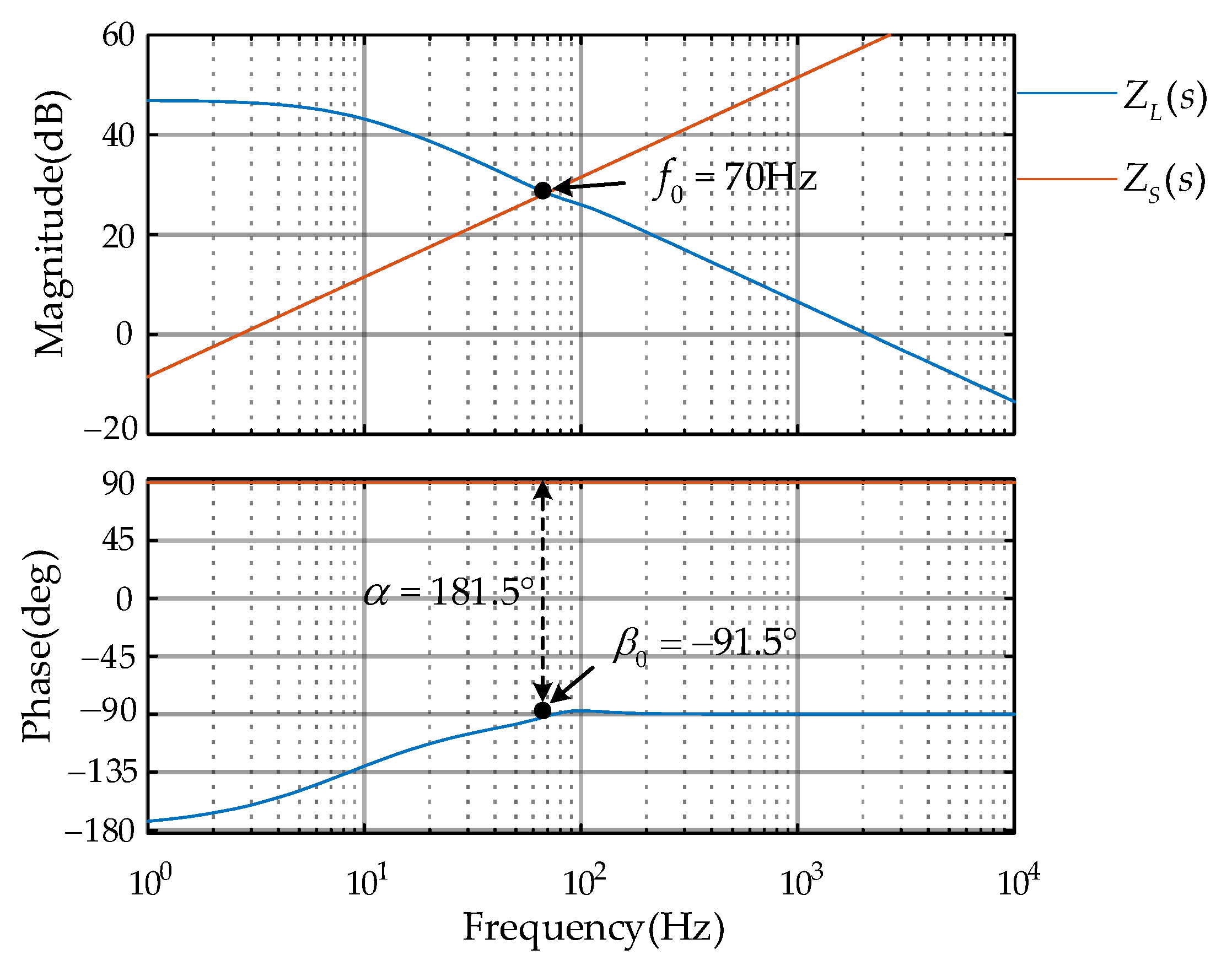
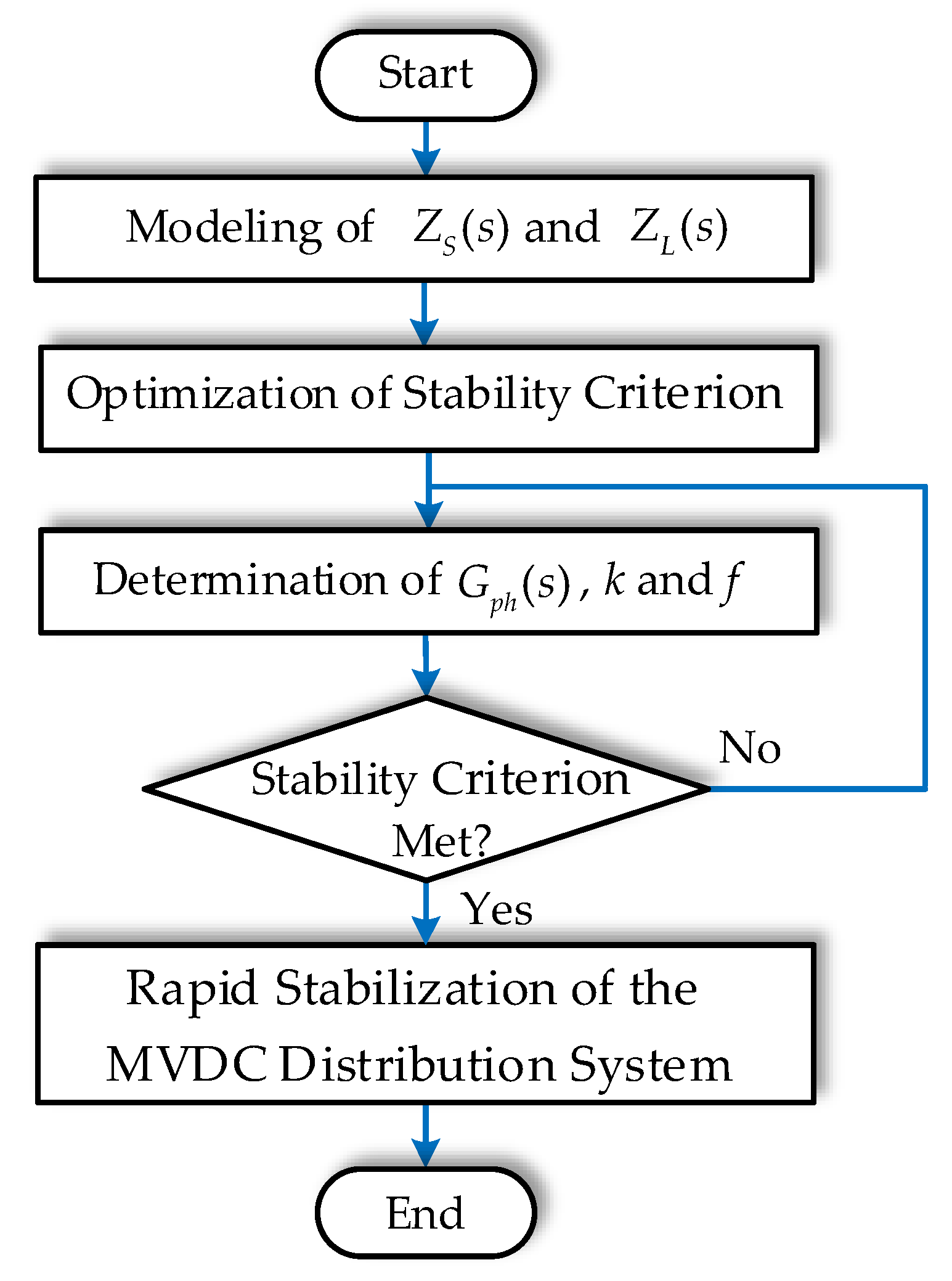
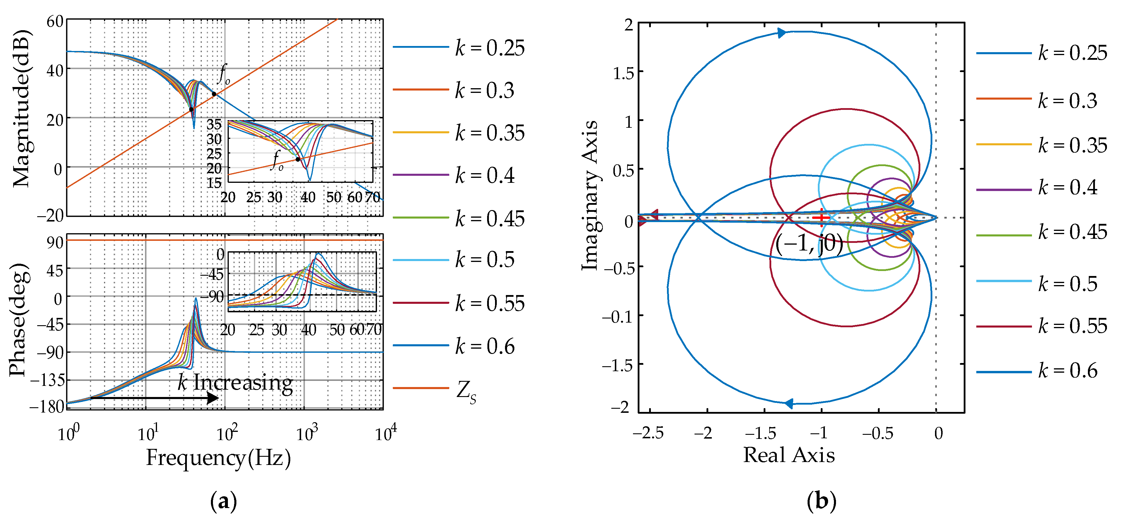
4.1. Optimization of the Stability Criterion

Since the analysis of Section 2 shows that the input impedance term generated by the input voltage sharing controllers is zero, the input voltage sharing loop transfer function $G_{u_M}(s)$ can be ignored. The small-signal block diagram of the i-th (i = 1, 2 … n) DAB converter with the impedance phase controller $G_{ph}(s)$ is shown in Figure 10.

According to (18) and Figure 10, the reshaped load impedance $Z_{L\_IPR}(s)$ can be calculated by

$$Z_{L\_IPR}(s)=n/[Y_{op}(s)+Y_{ci}(s)+\frac{G_{u_L{u}_{ini}}(s)G_{ph}(s)G_{u_L}(s)G_{i_{p}d}(s)}{1+G_{u_L}(s)G_{ph}(s)G_{u_{L}d}(s)}].$$

(23)

At the intersection of the source impedance amplitude and the load impedance amplitude, the load impedance $Z_{L\_IPR}(j{\omega }_0)$ can be expressed as

$$Z_{L\_IPR}(j{\omega }_0)=\left|Z_{L\_IPR}(j{\omega }_0)\right|e^{j\theta },$$

(24)

where θ is the phase of load impedance at the intersection, ${\omega }_0$ is the angular frequency of the intersection and ${\omega }_0=2\pi f_0$.

The traditional stability criterion is described as

$$\{\begin{array}{l}\left|Z_S(j{\omega }_0)\right|=\left|Z_L(j{\omega }_0)\right|,\\ \left|\arg \left[Z_S(j{\omega }_0)\right]-\arg \left[Z_L(j{\omega }_0)\right]\right|<{180}^{°}.\end{array}$$

(25)

In the MVDC distribution system, the phase of $Z_S(j{\omega }_0)$ is 90°. According to (25), the phase of the load impedance at $f_0$ should be satisfied θ ∈ (−90°, 270°).

To weaken the negative resistance characteristic of the ISOP DCT, the load impedance phase interval is optimized by narrowing θ ∈ (−90°, 0°). According to (24), the optimized stability criterion can be obtained as

$$\{\begin{array}{l}{\left|Z_{L\_IPR}(s)/Z_S(s)\right|}_{s=j{\omega }_0}=1,\\ -90^o<\theta <0^o.\end{array}$$

(26)

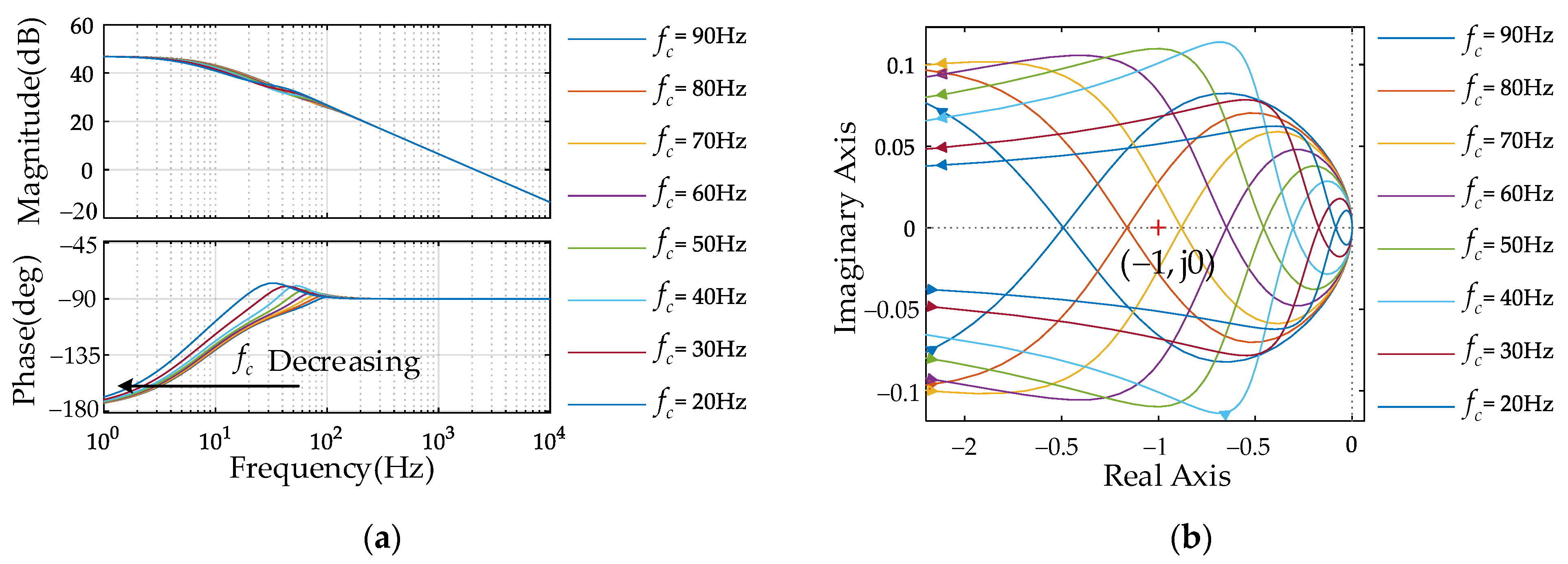
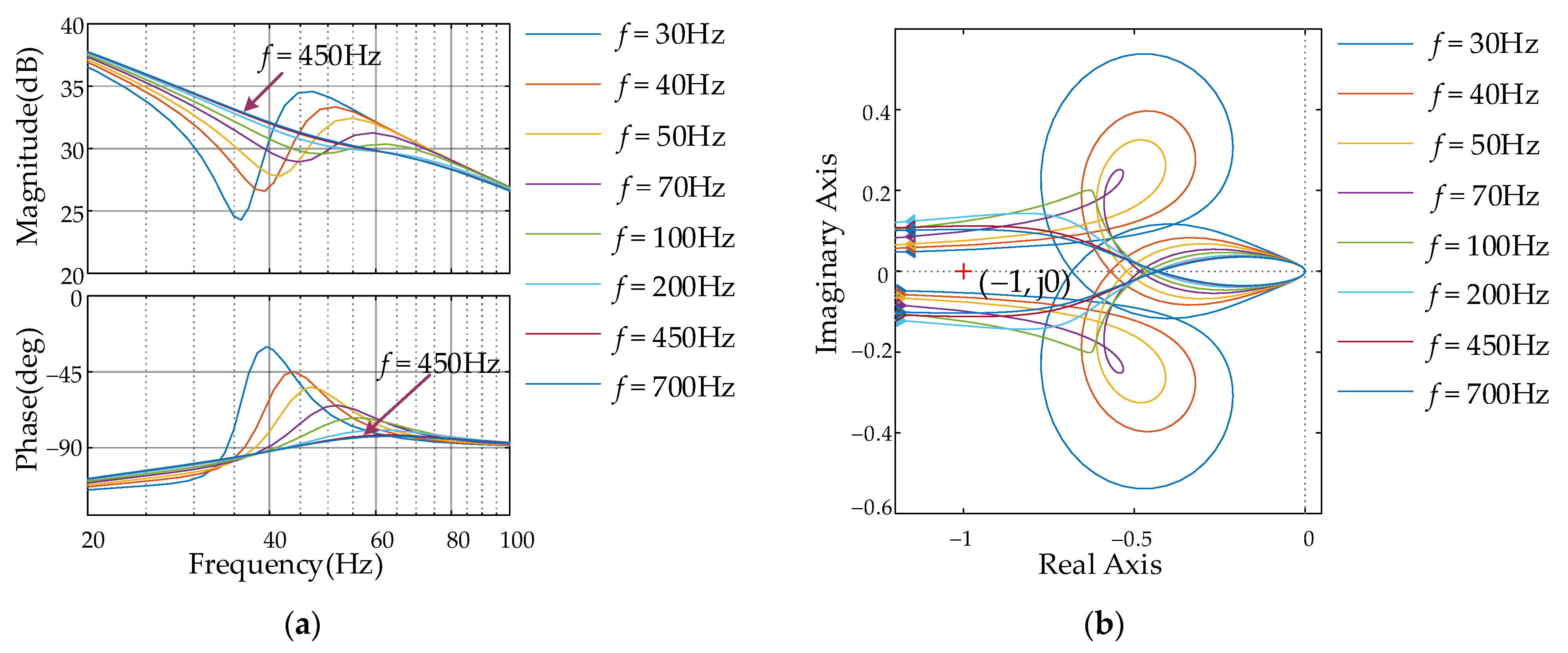
4.2. Design for the Impedance Phase Controller

As the order of the low-pass filter increases, the phase increases by 90° gradually. In this paper, a first-order low-pass filter is used to reshape the impedance phase at the intersection. The transfer function $G_{ph}(s)$ of the impedance phase controller can be expressed as

$$G_{ph}(s)=\frac{k\omega }{s+\omega },$$

(27)

$$\omega =2\pi f,$$

(28)

where ω and f are the cut-off angular frequency and cut-off frequency of the first-order low-pass filter, respectively. k is the gain of the impedance phase controller.

In this section, the determination of k and f is discussed. The constraint condition is to ensure that the intersecting impedance phase θ satisfies the optimized stability criterion in (26), while the amplitude is rarely affected. To analyze the influence of the gain k on the stability of the MV bus voltage, the initial cut-off frequency of the low-pass filter f is 30 Hz. The system stability analysis versus the gain k and cut-off frequency f are shown in Figure 11 and Figure 12.

From Figure 11a, we can see that with the increasing of k, the impedance phase is closer to 0° at low frequency. Since the negative resistance characteristic of $Z_{L\_IPR}(j{\omega }_0)$ is weakened, the stability of the MVDC distribution system is improved. However, the frequency band that satisfies the optimized stability criterion in (26) is narrowed. Meanwhile, with the increasing of k, the amplitude of $Z_{L\_IPR}(j{\omega }_0)$ changes obviously. When k > 0.5, the intersection frequency $f_0$ moves forward because of the amplitude change. Figure 11b shows that when k > 0.5, the Nyquist contour of the minor loop gain $T_m$ would encircle the point (−1, j0), so the MV bus voltage is unstable. When k = 0.5, the Nyquist contour of $T_m$ is close to the point (−1, j0). Therefore, the voltage tends to be unstable. While k = 0.45, the dynamic performance of the system is good, and the optimized stability criterion is satisfied.

It can be seen from Figure 12a that with the increase of cut-off frequency f, the impact on the amplitude becomes smaller and can be ignored. When f > 450 Hz, the phase and amplitude of $Z_{L\_IPR}(j{\omega }_0)$ are hardly changed. Figure 12b shows that none of the Nyquist contour of the minor loop gain $T_m$ encircles (−1, j0) when k = 0.45. Thus, the system remains stable with the increasing of f. When f = 450 Hz, the magnitude is hardly changed.

In summary, the proposed method can solve the instability problem of the MVDC distribution system by weakening the negative resistance characteristic of the load impedance. When the gain k = 0.45 and the cut-off frequency f = 450 Hz, the impedance satisfies the optimized stability criterion, resulting in the MV bus voltage oscillation being rapidly damped. Moreover, the impedance amplitude is rarely affected, and the dynamic performance of the system is good.

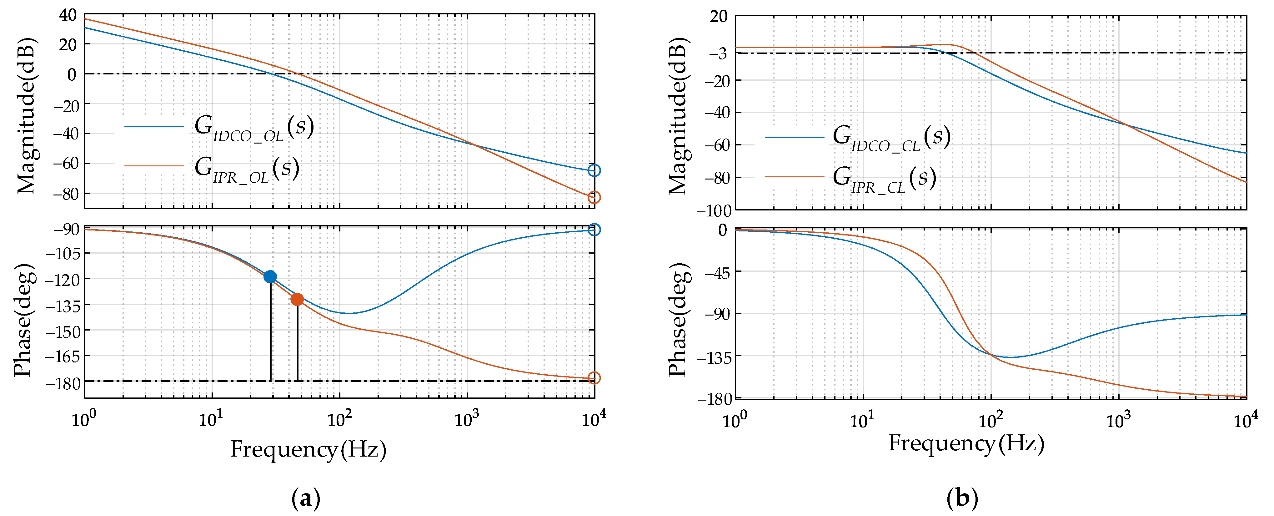
4.3. Comparison between the IDCO Method and IPR Method

4.3.1. Negative Resistance Characteristic of the Input Impedance for ISOP DCT

The negative impedance characteristics of the ISOP DCT may destabilize the system. At the impedance intersection $f_0$, the weakening of the negative impedance characteristic can suppress the bus voltage oscillation. Therefore, the suppression ability of the bus voltage oscillation based on the two methods can be evaluated by

$${\beta }_{IDCO}=\arg \left[Z_L(j\cdot 2\pi f_o)\right],$$

(29)

$${\beta }_{IPR}=arg\left[Z_{L\_IPR}(j\cdot 2\pi f_o)\right],$$

(30)

where ${\beta }_{IDCO}$ and ${\beta }_{IPR}$ are the phases of $Z_L(j\cdot 2\pi f_o)$ and $Z_{L\_IPR}(j\cdot 2\pi f_o)$, respectively. $Z_L(j\cdot 2\pi f_o)$ is the load impedance at $f_0$ based on the IDCO method and $Z_{L\_IPR}(j\cdot 2\pi f_o)$ is the load impedance at $f_0$ based on the IPR method.

Figure 7 shows that the impedance phase of the original system at $f_o$ is ${\beta }_0=-91.5°$. Substituting (18) and (23) into (29) and (30), respectively and combining the parameters in Table 1, ${\beta }_{IDCO}=-85°$ and ${\beta }_{IPR}=-83°$ can be obtained at $f_0=70Hz$. Both methods weaken the negative impedance characteristics of the ISOP DCT. However, the negative resistance characteristic of the load impedance based on the IPR method (${\beta }_{IPR}=-83°$) is weaker than that of the IDCO method (${\beta }_{IDCO}=-85°$), indicating that the system can achieve stability faster based on the IPR control.

4.3.2. Dynamic Performance of the MVDC Distribution System

The objective of the IDCO method and the IPR method is to improve the stability of the MVDC distribution system. Both can accomplish the goal by reshaping the load impedance as shown in Figure 8, Figure 11, and Figure 12. To further analyze the dynamic performance of the system, the voltage control closed-loop transfer functions are expressed as

$$G_{IDCO\_CL}(s)=\frac{G_{u_L}(s)G_{u_{L}d}(s)}{1+G_{u_L}(s)G_{u_{L}d}(s)},$$

(31)

$$G_{IPR\_CL}(s)=\frac{G_{u_L}(s)G_{ph}(s)G_{u_{L}d}(s)}{1+G_{u_L}(s)G_{ph}(s)G_{u_{L}d}(s)},$$

(32)

where $G_{IDCO\_CL}(s)$ is the voltage control closed-loop transfer function based on the IDCO method and $G_{IPR\_CL}(s)$ is the voltage control closed-loop transfer function based on the proposed IPR method.

The Bode diagram of $G_{IDCO\_OL}(s)$, $G_{IPR\_OL}(s)$, $G_{IDCO\_CL}(s)$, and $G_{IPR\_CL}(s)$ are shown in Figure 13, and the system parameters are listed in Table 1. $G_{IDCO\_OL}(s)$ and $G_{IPR\_OL}(s)$ are the output voltage control open-loop transfer functions, which are the numerator of (31) and (32), respectively. The comparisons between the IDCO method and the IPR method are summarized in

Table 2. Comparisons of the transfer functions.

	${\mathit{G}}_{\mathit{I}\mathit{D}\mathit{C}\mathit{O}\_\mathit{C}\mathit{L}}(\mathit{s})$	${\mathit{G}}_{\mathit{I}\mathit{P}\mathit{R}\_\mathit{C}\mathit{L}}(\mathit{s})$
Bandwidth	44 Hz	74 Hz
Phase Margin (PM)	60°	47°

.

As can be seen from Table 2, the bandwidth of $G_{IPR\_CL}(s)$ is 30 Hz greater than that of $G_{IDCO\_OL}(s)$. Thus, compared with the IDCO approach, the dynamic performance of the MVDC distribution system with the proposed method is better. Moreover, the PMs of both control methods are in the proper range, and the PM of the IDCO method is larger.

In conclusion, although the system stability is improved in both methods, the negative impedance characteristics of the system are weaker based on the IPR method. Therefore, the proposed IPR method could achieve the rapid stabilization of the MVDC distribution system. In addition, the bandwidth of the IPR method is larger than that of the IDCO method. Thus, the dynamic characteristics of the system are better. However, due to the small PM, the IPR method may produce a large overshoot in the dynamic process.

5. Simulation Results and Discussion

Based on the structure as shown in Figure 2, a 10 kV MVDC distribution system was built in MATLAB/Simulink. The ISOP DCT consists of three DAB modules, whose rated power P_r = 0.9 MW. The parameters of the simulation model are given in Table 1.

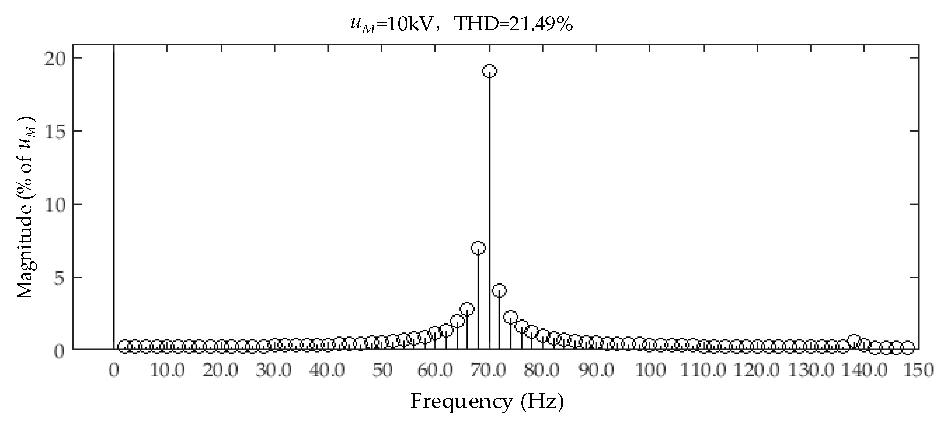
5.1. Verification of the Voltage Instability in the MVDC Distribution System

Fourier transform is a basic method in transform analysis from the time domain to the frequency domain. To verify the unstable problem of the MVDC distribution system, the MV bus voltage $u_M$ was analyzed by the fast Fourier transform (FFT) analysis function in MATLAB. The FFT analysis result of $u_M$ is illustrated in Figure 14. THD is the total harmonic distortion of $u_M$.

As can be seen from Figure 14, the oscillation frequency is mainly concentrated at 70 Hz and the THD is 21.49%. The results confirm that the original MVDC distribution system is unstable and the oscillation frequency of the MV bus voltage $u_M$ is consistent with Figure 7.

5.2. Verification of the Load Impedance Models

To verify the correctness of the developed impedance models, the bode diagrams of the analytical models are compared with the simulation results. The measurement method of the impedance simulation results is depicted in Figure 15. Moreover, the analytical modeling results and the simulation results of the load impedance are shown in Figure 16.

As shown in Figure 15, the sinusoidal perturbations ${\hat{u}}_f$ are superimposed on the MV bus. The frequency varies from 2 Hz to 10 kHz, and the peak amplitude of ${\hat{u}}_f$ is 500 V. Meanwhile, the disturbance current ${\hat{i}}_f$ is extracted by FFT analysis. The measured load impedance of the simulation system is expressed as

$$Z_L(s)=\frac{{\hat{u}}_f}{{\hat{i}}_f}.$$

(33)

From Figure 16, we can see that the analytical models match well with the measured results in the swept frequency range from 2 Hz to 10 kHz, indicating that the models expressed in (18) and (23) are accurate. Moreover, the proposed IPR method only changes the phase of $Z_{L\_IPR}(s)$ at 70 Hz and rarely affect the amplitude. The phase of $Z_{L\_IPR}(s)$ satisfies the phase interval in (26), which coincides with the proposed method.

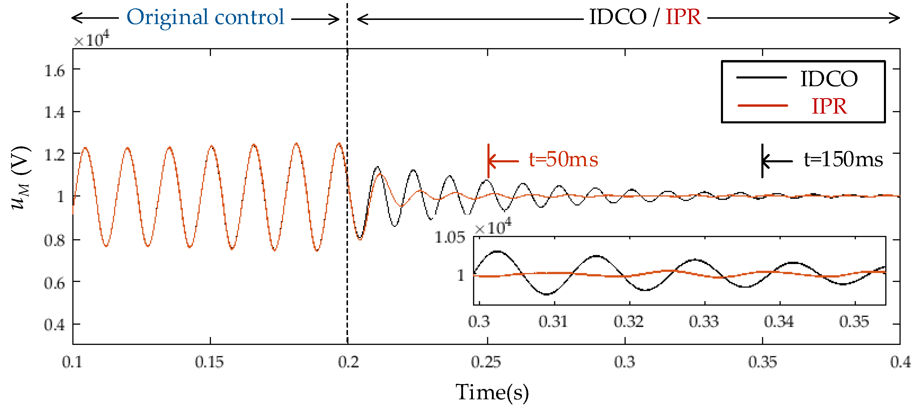
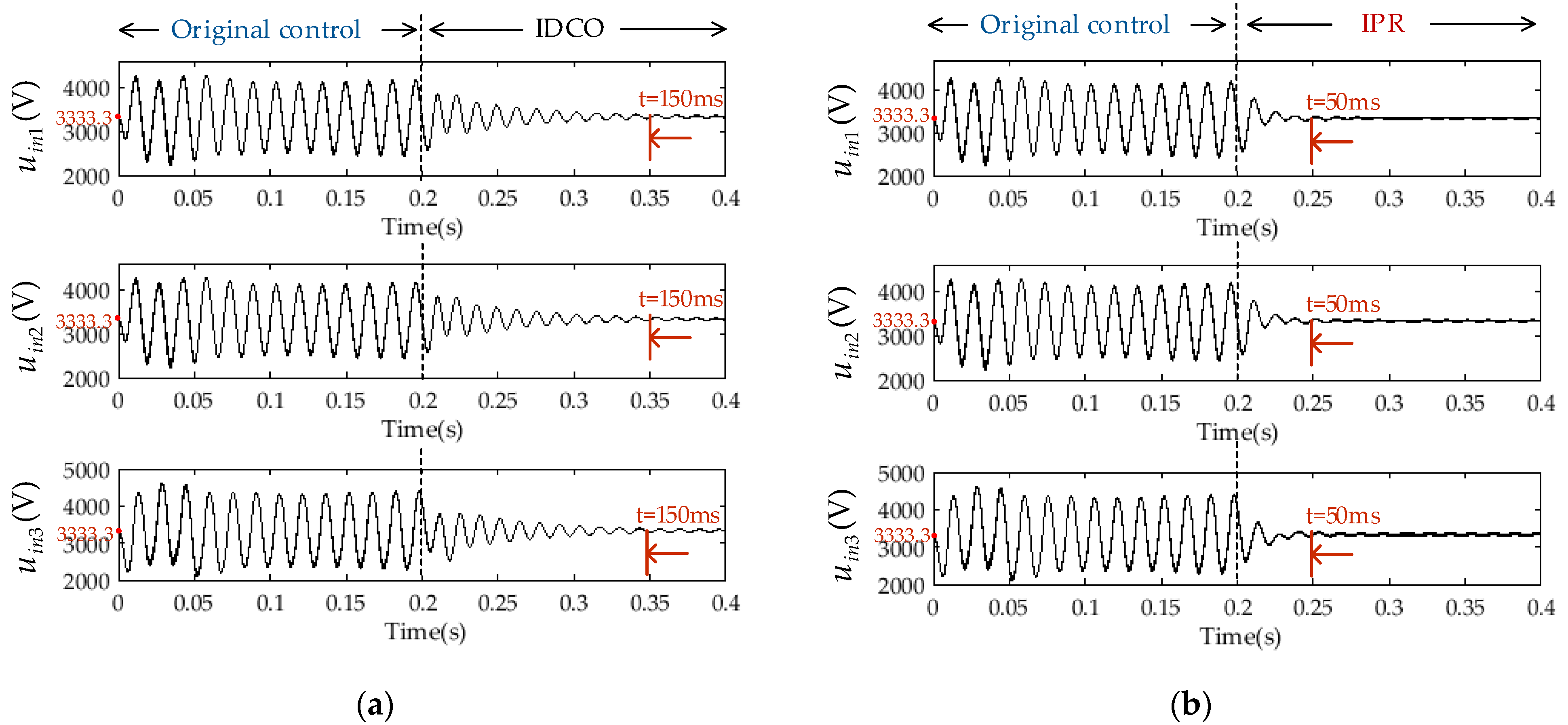
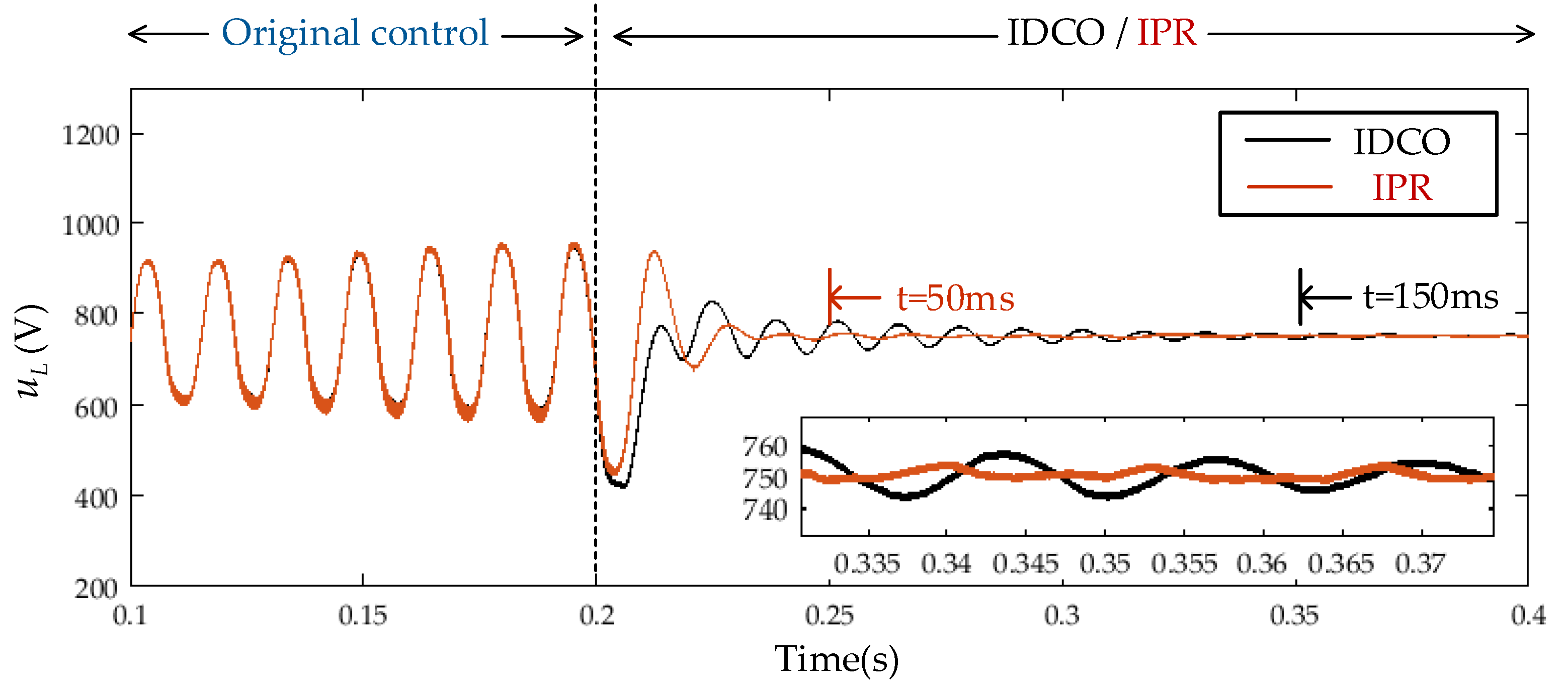
5.3. Verification of the IPR Method

The simulation model is tested under different working conditions to validate the proposed method. When t = 0.2, the system is switched from the original control to the IDCO control or the IPR control. When t = 0.5, the system changes from half load (p = 0.45 MW) to full load (p = 0.9 MW), i.e., the load steps from 1.25 Ω to 0.625 Ω. Besides, the reference value $u_L^{*}$ of the LV bus voltage steps from 100% ($u_L^{*}$ = 750 V) to 80% ($u_L^{*}$ = 600 V) at t = 0.7 s. The damping ability to bus voltage oscillation of these two methods is illustrated in Figure 17, Figure 18 and Figure 19. The dynamic performance of the MVDC distribution system is shown in Figure 20, Figure 21 and Figure 22.

From Figure 17, we can see that for the IDCO and the IPR method, the oscillation of the MV bus voltage $u_M$ is suppressed within 150 ms and 50 ms, respectively. This confirms that the IPR method rapidly suppresses the MV bus voltage oscillation. Moreover, the ripple of $u_M$ using the proposed IPR method is smaller than that of the IDCO approach, because the negative resistance characteristic of the ISOP DCT is weakened.

In the observation from Figure 18a,b, the DAB modules voltage $u_{in1}$, $u_{in2}$, and $u_{in3}$ are stable at 3333.3 V. The simulation results demonstrate that the ISOP DCT achieves input voltage sharing. It indicates that the input voltage sharing controller optimization could be ignored, which is consistent with Figure 10. In addition, the transient period of the proposed IPR method is 100 ms shorter than that of the IDCO method. These results indicate that the proposed method can stabilize the voltage faster.

As shown in Figure 19, when the IPR controller is activated, the stabilization time of the LV bus voltage $u_L$ is reduced from 150 ms to 50 ms. This validates that the proposed method is effective. The voltage ripple rate of $u_L$ with the proposed method (about 2%) is lower than that of the IDCO approach (about 2.7%). This illustrates that compared with the IDCO method, the waveform quality based on the IPR method is significantly better. This also indicates that the impedance phase satisfies the phase interval, which further weakens the negative resistance characteristic of the load impedance.

As can be seen from Figure 20, the transient recovery time of the proposed IPR method is 60 ms, which is faster than that of the IDCO approach (about 80 ms). Although the ripple rates are both less than 1%, the result shows that the voltage is more stable with the proposed IPR method than the IDCO method. This validates the effectiveness of the proposed method at the full-load condition. Furthermore, the dynamic performance is good due to the proper bandwidth and phase margin as shown in Table 2.

The waveforms of the LV bus voltage $u_L$ also confirm the good dynamic performance of the IPR method as shown in Figure 21 and Figure 22. It is evident that $u_L$ tracks the step reference well as shown in Figure 21, and the corresponding transient voltage has a short settling time (40 ms). As can be seen from Figure 22, the overshoot of $u_L$ with the proposed IPR control approach is 25 V and the overshoot rate is 4%. It can be seen from Figure 21 and Figure 22 that compared with the IDCO method, the overshoot based on the IPR control is larger, but is still within a reasonable range. These results validate the robustness and effectiveness of the proposed control.

6. Conclusions

This paper proposes an IPR method to rapidly stabilize the MVDC distribution system. Based on the obtained load impedance model, the 10 kV MVDC distribution system using the traditional IDCO method and the proposed IPR method was analyzed and simulated. The following relevant conclusions were obtained:

(i)

Due to the decoupling condition of the control strategy for the ISOP DCT, the load impedance is hardly affected by the input voltage sharing controller optimization.

(ii)

Compared with the IDCO method, the proposed method further weakens the negative resistance characteristic of the ISOP DCT and suppresses the voltage oscillation rapidly. Moreover, regardless of load step-change or voltage reference step-change, the proposed method has a good dynamic performance and stability for the system. The overshoot of the proposed IPR method is larger than that of the traditional IDCO method, but it is still reasonable. This is a tradeoff for the rapid stabilization of the MVDC distribution systems.

(iii)

Compared with the method of modifying the impedance amplitude, the proposed IPR method considers the problem that the amplitude must intersect. The phase interval of the optimized stability criterion is adjustable. Furthermore, the impedance phase controller can be designed by the high order low-pass filter and bandpass filter, which are flexible and can be applied to the stability analysis for other systems.

References

1. Baran, M.E.; Mahajan, N.R. DC distribution for industrial systems: Opportunities and challenges. IEEE Trans. Ind. Appl. 2003, 39, 1596–1601. [Google Scholar] [CrossRef]
2. Simiyu, P.; Xin, A.; Wang, K.; Adwek, G.; Salman, S. Multiterminal medium voltage DC distribution network hierarchical control. Electronics 2020, 9, 506. [Google Scholar] [CrossRef] [Green Version]
3. Huang, A.Q.; Crow, M.L.; Heydt, G.T.; Zheng, J.P.; Dale, S.J. The future renewable electric energy delivery and management (FREEDM) system: The energy internet. Proc. IEEE 2011, 99, 133–148. [Google Scholar] [CrossRef]
4. Mura, F.; De Doncker, R.W. Design aspects of a medium-voltage direct current (MVDC) grid for a university campus. In Proceedings of the 8th International Conference on Power Electronics—ECCE Asia, Jeju, Korea, 30 May–3 June 2011. [Google Scholar]
5. Steimel, A. Under europe’s incompatible catenary voltages a review of multi-system traction technology. In Proceedings of the 2012 Electrical Systems for Aircraft, Railway and Ship Propulsion, Bologna, Italy, 16–18 October 2012. [Google Scholar]
6. Verdicchio, A.; Ladoux, P.; Caron, H.; Courtois, C. New medium-voltage DC railway electrification system. IEEE Trans. Transp. Electrif. 2018, 4, 591–604. [Google Scholar] [CrossRef]
7. Zhu, R.; Liang, T.; Dinavahi, V.; Liang, G. Wideband modeling of power SiC mosfet module and conducted EMI prediction of MVDC railway electrification system. IEEE Trans. Electromagn. Compat. 2020, 62, 2621–2633. [Google Scholar] [CrossRef]
8. Castellan, S.; Menis, R.; Tessarolo, A.; Sulligoi, G. Power electronics for all-electric ships with MVDC power distribution system: An overview. In Proceedings of the 2014 Ninth International Conference on Ecological Vehicles and Renewable Energies (EVER), Monte-Carlo, Monaco, 25–27 March 2014. [Google Scholar]
9. Li, Z.; Liang, S.; Ren, L.; Tan, X.; Xu, Y.; Tang, Y.; Li, J.; Shi, J. Application of flux-coupling-type superconducting fault current limiter on shipboard MVDC integrated power system. IEEE Trans. Appl. Supercond. 2020, 30, 1–8. [Google Scholar] [CrossRef]
10. Javaid, U.; Freijedo, F.D.; Dujic, D.; van der Merwe, W. MVDC supply technologies for marine electrical distribution systems. CPSS Trans. Power Electron. Appl. 2018, 3, 65–76. [Google Scholar] [CrossRef]
11. Tu, H.; Feng, H.; Srdic, S.; Lukic, S. Extreme fast charging of electric vehicles: A technology overview. IEEE Trans. Transp. Electrif. 2019, 5, 861–878. [Google Scholar] [CrossRef]
12. Mohammadpour, A.; Parsa, L.; Todorovic, M.H.; Lai, R.; Datta, R.; Garces, L. Series-input parallel-output modular-phase DC–DC converter with soft-switching and high-frequency isolation. IEEE Trans. Power Electron. 2016, 31, 111–119. [Google Scholar] [CrossRef]
13. Zumel, P.; Ortega, L.; Lázaro, A.; Fernández, C.; Barrado, A.; Rodríguez, A.; Hernando, M.M. Modular dual-active bridge converter architecture. IEEE Trans. Ind. Appl. 2016, 52, 2444–2455. [Google Scholar] [CrossRef] [Green Version]
14. Ruan, X.; Chen, W.; Cheng, L.; Tse, C.K.; Yan, H.; Zhang, T. Control strategy for input-series–output-parallel converters. IEEE Trans. Ind. Electron. 2009, 56, 1174–1185. [Google Scholar] [CrossRef]
15. Grigore, V.; Hatonen, J.; Kyyra, J.; Suntio, T. Dynamics of a buck converter with a constant power load. In Proceedings of the PESC 98 Record. In Proceedings of the 29th Annual IEEE Power Electronics Specialists Conference (Cat. No.98CH36196), Fukuoka, Japan, 22–22 May 1998. [Google Scholar]
16. Du, W.; Zhang, J.; Zhang, Y.; Qian, Z. Stability criterion for cascaded system with constant power load. IEEE Trans. Power Electron. 2013, 28, 1843–1851. [Google Scholar] [CrossRef]
17. Su, M.; Liu, Z.; Sun, Y.; Han, H.; Hou, X. stability analysis and stabilization methods of dc microgrid with multiple parallel-connected DC–DC converters loaded by CPLs. IEEE Trans. Smart Grid 2018, 9, 132–142. [Google Scholar] [CrossRef]
18. Emadi, A.; Khaligh, A.; Rivetta, C.H.; Williamson, G.A. Constant power loads and negative resistance instability in automotive systems: Definition, modeling, stability, and control of power electronic converters and motor drives. IEEE Trans. Veh. Technol. 2006, 55, 1112–1125. [Google Scholar] [CrossRef]
19. Javaid, U.; Freijedo, F.D.; Dujic, D.; van der Merwe, W. Dynamic assessment of source–load interactions in marine MVDC distribution. IEEE Trans. Ind. Electron. 2017, 64, 4372–4381. [Google Scholar] [CrossRef]
20. Liu, H.; Xie, X.; He, J.; Xu, T.; Yu, Z.; Wang, C.; Zhang, C. Subsynchronous interaction between direct-drive PMSG based wind farms and weak AC networks. IEEE Trans. Power Syst. 2017, 32, 4708–4720. [Google Scholar] [CrossRef]
21. Li, C. Unstable operation of photovoltaic inverter from field experiences. IEEE Trans. Power Deliv. 2018, 33, 1013–1015. [Google Scholar] [CrossRef]
22. Qin, H.; Kimball, J.W. Generalized average modeling of dual active bridge DC–DC converter. IEEE Trans. Power Electron. 2012, 27, 2078–2084. [Google Scholar]
23. Singh, B.; Shankar, G.; Singh, A. Modelling of inverter interfaced dual active bridge converter. In Proceedings of the 2018 International Conference on Computing, Power and Communication Technologies (GUCON), Greater Noida, India, 28–29 September 2018. [Google Scholar]
24. Mueller, J.A.; Kimball, J.W. Model-based determination of closed-loop input impedance for dual active bridge converters. In Proceedings of the 2017 IEEE Applied Power Electronics Conference and Exposition (APEC), Tampa, FL, USA, 26–30 March 2017. [Google Scholar]
25. Ye, Q.; Mo, R.; Li, H. Stability analysis and improvement of a dual active bridge (DAB) converter enabled DC microgrid based on a reduced-order low frequency model. In Proceedings of the 2016 IEEE Energy Conversion Congress and Exposition (ECCE), Milwaukee, WI, USA, 18–22 September 2016. [Google Scholar]
26. Middlebrook, R.D.; Cuk, S. A general unified approach to modelling switching-converter power stages. In Proceedings of the 1976 IEEE Power Electronics Specialists Conference, Cleveland, OH, USA, 8–10 June 1976. [Google Scholar]
27. Sun, J. Impedance-based stability criterion for grid-connected inverters. IEEE Trans. Power Electron. 2011, 26, 3075–3078. [Google Scholar] [CrossRef]
28. Riccobono, A.; Santi, E. Comprehensive review of stability criteria for DC power distribution systems. IEEE Trans. Ind. Appl. 2014, 50, 3525–3535. [Google Scholar] [CrossRef]
29. Zhong, Q.; Zhang, X. Impedance-sum stability criterion for power electronic systems with two converters/sources. IEEE Access 2019, 7, 21254–21265. [Google Scholar] [CrossRef]
30. Wang, X.; Qing, H.; Huang, P.; Zhang, C. Modeling and stability analysis of parallel inverters in island microgrid. Electronics 2020, 9, 463. [Google Scholar] [CrossRef] [Green Version]
31. Riccobono, A.; Santi, E. A novel passivity-based stability criterion (PBSC) for switching converter DC distribution systems. In Proceedings of the 2012 Twenty-Seventh Annual IEEE Applied Power Electronics Conference and Exposition (APEC), Orlando, FL, USA, 5–9 February 2012. [Google Scholar]
32. Riccobono, A.; Santi, E. Stability analysis of an all-electric ship MVDC power distribution system using a novel passivity-based stability criterion. In Proceedings of the 2013 IEEE Electric Ship Technologies Symposium (ESTS), Arlington, VA, USA, 22–24 April 2013. [Google Scholar]
33. Zhu, X.; Hu, H.; Tao, H.; He, Z. Stability analysis of PV plant-tied MVDC railway electrification system. IEEE Trans. Transp. Electrif. 2019, 5, 311–323. [Google Scholar] [CrossRef]
34. Feng, F.; Wu, F.; Gooi, H.B. Impedance shaping of isolated two-stage AC-DC-DC converter for stability improvement. IEEE Access 2019, 7, 18601–18610. [Google Scholar] [CrossRef]
35. Abdollahi, H.; Arrua, S.; Roinila, T.; Santi, E. A novel DC power distribution system stabilization method based on adaptive resonance-enhanced voltage controller. IEEE Trans. Ind. Electron. 2019, 66, 5653–5662. [Google Scholar] [CrossRef]
36. Zhang, X.; Ruan, X.; Zhong, Q. Improving the stability of cascaded DC/DC converter systems via shaping the input impedance of the load converter with a parallel or series virtual impedance. IEEE Trans. Ind. Electron. 2015, 62, 7499–7512. [Google Scholar] [CrossRef]
37. Feng, F.; Zhang, X.; Zhang, J.; Gooi, H.B. Stability enhancement via controller optimization and impedance shaping for dual active bridge-based energy storage systems. IEEE Trans. Ind. Electron. 2021, 68, 5863–5874. [Google Scholar] [CrossRef]
38. Guan, Y.; Xie, Y.; Wang, Y.; Liang, Y.; Wang, X. An active damping strategy for input impedance of bidirectional dual active bridge DC–DC converter: Modeling, shaping, design, and Experiment. IEEE Trans. Ind. Electron. 2021, 68, 1263–1274. [Google Scholar] [CrossRef]
39. Wang, Y.; Guan, Y.; Fosso, O.B.; Molinas, M.; Chen, S.; Zhang, Y. An input-voltage-sharing control strategy of input-series-output-parallel isolated bidirectional DC/DC converter for dc distribution network. IEEE Trans. Power Electron. 2022, 37, 1592–1604. [Google Scholar] [CrossRef]
Figure 1. A typical DC distribution system.
Electronics 10 03163 g001
Figure 2. Structure of the MVDC distribution system.
Electronics 10 03163 g002
Figure 3. Control block diagram of the ISOP DCT.
Electronics 10 03163 g003
Figure 4. Control block diagram of the i-th (i = 1, 2 … n − 1) DAB module.
Electronics 10 03163 g004
Figure 5. Control block diagram of the n-th DAB converter.
Electronics 10 03163 g005
Figure 6. Inter connection of the sub-system for the MVDC distribution system.
Electronics 10 03163 g006
Figure 7. Bode diagram of Z S ( s ) and Z L ( s ) .
Electronics 10 03163 g007
Figure 8. MVDC distribution system stability analysis with different cut-off frequencies: (a) Bode diagram of Z L ( s ) , (b) Nyquist diagram of T m .
Electronics 10 03163 g008
Figure 9. Flowchart of the proposed IPR method.
Electronics 10 03163 g009
Figure 10. Small-signal block diagram of DAB with G p h ( s ) .
Electronics 10 03163 g010
Figure 11. Stability analysis of the MVDC distribution system: (a) Bode diagram of Z L _ I P R ( j ω 0 ) , (b) Nyquist diagram of T m .
Electronics 10 03163 g011
Figure 12. Stability analysis of the MVDC distribution system: (a) Bode diagram of Z L _ I P R ( s ) , (b) Nyquist diagram of T m .
Electronics 10 03163 g012
Figure 13. Bode diagram of the transfer functions based on the IDCO method and the proposed IPR method: (a) open-loop transfer functions, (b) closed-loop transfer functions.
Electronics 10 03163 g013
Figure 14. FFT analysis of the MV bus voltage u M .
Electronics 10 03163 g014
Figure 15. Impedance measurement by the disturbance injection method.
Electronics 10 03163 g015
Figure 16. Bode diagram of the load impedance: (a) input impedance Z L ( s ) based on the IDCO method, (b) input impedance Z L _ I P R ( s ) based on the proposed IPR method.
Electronics 10 03163 g016
Figure 17. Damping results of the MV bus voltage u M .
Electronics 10 03163 g017
Figure 18. Input voltage of three DAB modules: (a) IDCO method, (b) proposed IPR method.
Electronics 10 03163 g018
Figure 19. Damping results of the LV bus voltage u L .
Electronics 10 03163 g019
Figure 20. Dynamic waveforms of the MV bus voltage u M based on the IDCO or IPR control method under a load step-change.
Electronics 10 03163 g020
Figure 21. Dynamic waveforms of the LV bus voltage u L based on the IDCO or IPR control method under a load step-change.
Electronics 10 03163 g021
Figure 22. Dynamic waveforms of the LV bus voltage u L based on the IDCO or IPR control method under a reference value step-change.
Electronics 10 03163 g022