Research on the Cross-Platform Co-Simulation Strategy of Power Systems Based on the Model-Segmentation Algorithm

Abstract

In recent years, cross-platform co-simulation has become an important development direction of the real-time simulation of power systems. Model segmentation is at the core of the realization of cross-platform joint simulation and parallel real-time simulation of these systems. In essence, it is based on the deep application of a system-decoupling algorithm. In order to solve problems that a single interface cannot, it considers the data interaction of large- and small-step systems at the same time This paper proposes an improved joint-simulation strategy based on the model-segmentation method for the cross-platform joint-simulation technology of a large-scale, flexible direct-power grid sent by the wind farms of RT-lab and Hypersim. Firstly, by studying several common interface algorithms in the current project, the adaptability of different interface algorithms is analyzed. Secondly, the problem of high-frequency oscillation caused by the inductance-decoupling algorithm is improved, and an improved segmentation-model algorithm is proposed. Finally, according to the adaptability, each interface algorithm is applied to the wind-power-based, flexible direct-transmission, dual-platform simulation model that was built for this study. The simulation results verify the feasibility of the improved interface in system decoupling and platform interfacing, and indicate the significantly improved accuracy and stability of the system.

1. Introduction

At present, real-time simulation plays an important role in the experimental research, planning and design, operation scheduling, equipment research and development, control and protection, etc., of power systems [1,2,3,4]. Among them, electromagnetic transient real-time simulation is one of the technical means that is often used to study the dynamic characteristics of power systems, but the calculation step of the electromagnetic transient simulation is small (μs); when the number of system nodes or converter stations that are studied is large, the amount of calculation will greatly increase and the memory and processing overhead will be large, which often leads to processor overload or memory overflow, resulting in calculation failure. In recent years, with the development of the AC/DC power-grid interconnection, the distributed energy-grid connection and the flexible DC transmission, the simulation scale of power systems continues to expand. The impact of the new large-scale energy-grid connection on the power grid is the focus of current power-simulation research. At present, almost all of the focus is on simulating the AC/DC power grid and the new energy under a single simulation platform [5]. This causes two problems: one is the limitation of the simulation scale, and the other is that a single simulation platform has difficulty simultaneously considering the complexity of large-scale AC/DC power grids and the power electronic characteristics of the new energy equipment.

With the development of the large-scale power system, the control strategy and internal structure of the whole grid are more complex than before. Hence, the requirements for the real-time system simulation of the power system are more and more complex. It roughly develops from the following two directions. One of them is the requirement for simulation accuracy at the millisecond level to microsecond level, and even the nanosecond level has been used in some industries such as aerospace. The improvement of the accuracy introduces significant challenges to the hardware performance (such as the CPU) of the simulation platform. In order to avoid these problems, the research on a multi-machine co-simulation platform with a distributed parallel-simulation performance has become another promising development direction [6]. Both of the above development methods need to rely on hardware-in-loop (HIL) technology. Hardware-in-loop simulation can be used to verify the effectiveness of the power-system-control strategy and the correctness of the protection device action, which is beneficial to the R&D of the product. However, all HIL-based research must be based on real-time simulation. The complexity of the model calculation determines the speed of the simulation. To achieve real-time simulation, the simulation hardware should complete all of the calculation tasks within one step. Given the hardware, whether real-time simulation can be achieved is almost always determined by the modeling technology [7].

It is difficult for a single simulation platform to simultaneously consider the modeling of large-scale and complex AC/DC grids and the high-precision simulation of power electronic devices. As a result, multi-platform co-simulation and synchronous communication strategy between platforms have become important research aspects in the development of the real-time simulation of large-scale power systems. In order to solve this problem, there have been studies aimed at the co-simulation method, including one that proposed two methods for the dynamic co-simulation of CoTDS using parallel and series computations of the transmission system and distribution systems, and the results are a step forward in determining the appropriate integration-time step and the co-simulation computation method for numerical convergence [8]. Another study introduced a tightly-coupled (TC) protocol that used the serial method (SM) for solution exchange between the T&D systems [9]. This approach was shown to be computationally efficient compared to the parallel method (PM) of exchanging T&D system solutions. The above methods studied the communication interaction from the perspective of the interface selection. However, the requirements for the system hardware are still strict. Hence, a new co-simulation method is proposed, known as the model-segmentation algorithm, and is becoming one of the more effective methods for solving the real-time-simulation problem of large power grids.

The model-segmentation algorithm is based on the idea of division into space groups. A larger system is divided into several subsystems, and a state-space system is divided into two or more state-space groups. Each state-space group has its own state space. Matrix calculation greatly shortens the calculation time. In addition, the split-core parallel computing based on the segmentation model can greatly reduce the computational burden on a processor and increase the simulation scale. This algorithm becomes an effective way to perform large-scale real-time simulation.

There are some studies on the model-segmentation algorithm in academic and industrial fields. One study described an improved decoupled algorithm in the parallel real-time simulation of large-scale wind power systems and modular multi-level converters based on the RT-lab platform that has a high simulation accuracy, but the CPU utility cannot control in a suitable range [10,11]. Another study uses a model-partition method to perform parallel calculations on AC/DC power systems, which also greatly accelerates the calculation speed [12,13]. On the basis of the stability characteristics of the ideal transformer, one study proposed a model-segmentation interface-conversion algorithm, which makes the segmentation interface universal in the distribution network [14]. However, the above methods indicate that a single interface algorithm cannot simultaneously consider the data interactions of large- and small-step systems, the stability of the interface algorithm under different circuit topologies, and the universality of the compensation algorithm. In summary, this paper proposes a dual-platform simulation architecture of RT-lab and Hypersim based on multi-interface algorithms. The system is decoupled and reduced at the platform interface and inside the systems on both sides, through appropriate interface algorithms, in order to achieve real-time simulation.

The specific contributions of this work are detailed below.

• Comparison of the interface algorithm: different methods of system coupling are compared for their accuracy in modeling the integrated power system for real-time-simulation studies of different integration scenarios.
• Improvement of short-line (inductance) decoupling method: we introduce an improved short-line decoupling method for the co-platform system segmentation. This approach is shown to be computationally efficient compared to the existing short-line decoupling method of power system solutions that was used in our previous work.
• Co-simulation platform structure: a co-simulation platform is built for simulation testing by using the model-segmentation algorithm with the improved decoupling method. It is validated that the proposed co-simulation platform structure is suitable for bulk power systems and has high accuracy, and that the improved interface algorithm has a lower occupancy of resources than before.

2. Interface Algorithm

The decoupling principle of co-simulation is to use the waveguide-delay characteristics of the transmission line. Figure 1 shows the Bergeron equivalent circuit diagram of the transmission line. A transmission line can be split into two independent current-injection two-port networks. This model is called the Distributed Parameters Line (DPL). When performing simulation modeling, decoupling the inductance L of the system or line can be equivalent to the circuit in the Figure 1, where Ts is the simulation step size, L is the equivalent front reactance value, and K and R are the equivalent inductances, etc. The value is obtained after the effect.

There are four widely used interface algorithms for engineering applications: transmission-line-decoupling algorithms, ideal-transformer-model algorithms, short-line (inductance)-decoupling algorithms, and the space-state method [15,16]. This section analyzes and derives the above four interface algorithms.

2.1. Transmission-Line-Decoupling Algorithms

The principle of transmission-line decoupling is based on the inherent delay of electromagnetic waves in a line transmission to achieve natural decoupling. When the transmission delay t of the wave on the line is greater than the simulation step or the delay of the dual platform, the tasks at both ends of the line can be divided into two systems for calculation [12].

For a transmission line, after neglecting its loss, the wave equation of an electromagnetic wave can be obtained as:

$$\begin{array}{l}-\frac{\partial u}{\partial x}=L\frac{\partial i}{\partial t}\\ -\frac{\partial i}{\partial x}=L\frac{\partial u}{\partial t}\end{array}$$

(1)

The above formula has a d’Alembert solution

$$\{\begin{array}{c}i=f_1(x-vt)+f_2(x+vt)\\ u=Z_C{f}_1(x-vt)+Z_C{f}_2(x+vt)\end{array}$$

(2)

where f₁(x − vt) and f₂(x + vt) are functions of and x − vt and x + vt, respectively, which represent the inductance and capacitance of the traveling wave propagating in the positive direction and the reverse direction of km at speed v, and l and C are unit length. The traveling wave transmission speed v = 1/√LC, Z_C = √L/C is wave impedance.

Formula (3) can be obtained from the Formula (2)

$$\{\begin{array}{l}u+Z_{C}i=2Z_C{f}_1(x-vt)\\ u-Z_{C}i=2Z_C{f}_2(x-vt)\end{array}$$

(3)

while x − vt and x + vt are constant, the value of u + Z_Ci or u − Z_Ci is constant. Let the time of the traveling wave from the k-end to the m-end be τ = l/v.

Formula (4) is the expression of the time relationship between voltage and current at both ends of k and m:

$$u\left(k,t-\pi \right)+Z_C{i}_{km}\left(k,t-\pi \right)=u\left(m,t\right)+Z_C{i}_{km}\left(m,t\right)$$

(4)

and,

$$i_{mk}(m,t)=\frac{1}{Z_C}u(m,t)+I_{khis}$$

(5)

$$I_{khis}=-i_{km}(k,t-\tau )-\frac{1}{Z_C}u(k,t-\tau )$$

(6)

Similarly,

$$i_{km}(k,t)=\frac{1}{Z_C}u(k,t)+I_{mhis}$$

(7)

$$I_{mhis}=-i_{mk}(k,t-\tau )-\frac{1}{Z_C}u(m,t-\tau )$$

(8)

Figure 1 shows that the equivalent model of a lossless single-phase distributed parameter line is obtained.

When the long-transmission-line-decoupling method is used for model-segmentation calculation, each simulation step only needs to transmit the node voltage on each side of the transmission line, the communication volume is small, the model segmentation is processed by using the characteristics of the line, and there is no numerical instability problem. However, it can only be carried out on long-distance distributed parameter lines, and the actual system is sometimes difficult to meet the requirements, so this segmentation method has poor flexibility [13].

2.2. Short-Line (Inductance) Decoupling Algorithms

The transmission line decoupling algorithms has high requirements for the line length and ignores the resistance. This decoupling method is more applicable in the transmission network, because in the transmission network, the line length is generally long, which can reach more than hundreds of kilometers, and the voltage-level is high. The line resistance is far less than the inductance, which is not an order of magnitude, the existence of resistance can be ignored.

However, in the type of short distance line (such as distribution network), the voltage-level usually in a low range, the resistance and inductance are in the same order of magnitude, and the existence of resistance cannot be ignored. Moreover, the lines in this type of network are generally short, and the line length cannot meet the minimum requirements of distributed parameter lines. According to the transmission principle of a distributed parameter line, the minimum decoupling distributed-parameter-line length is 15 km [14]. The simulation results may not converge while using transmission-line-decoupling algorithms. Hence, the method of decoupling the short line is proposed.

The principle of inductance decoupling is to solve the transient network equation of inductance by using the trapezoidal integral law. Figure 2 shows the equivalent mathematical model of inductance.

For the terminal voltage u_k, um, the voltage inductance L is shown in Equation (9)

$$u_L=L\frac{d{i}_{km}(t)}{dt}=u_k-u_m$$

(9)

It is obtained from the state known at the current time in Formula (9)

$$i_{km}(t)=i_{km}(t-\Delta t)+\frac{1}{L}{\displaystyle {\int }_{t-\Delta t}^t{u}_k-u_m}$$

(10)

Formulas (11) and (12) can be obtained by using the trapezoidal-integration algorithm for Formula (10)

$$i_{km}(t)=\frac{\Delta t}{2L}\left\{{(u_k-u_m)}_t+{(u_k-u_m)}_{t-\Delta t}\right\}+i_{km}$$

(11)

$$i_{km}(t)=\frac{1}{R_1}{(u_k-u_m)}_t+I_{km}(t-\Delta t)$$

(12)

where

$$I_{km}(t-\Delta t)=\frac{1}{R_1}{(u_k-u_m)}_{t-\Delta t}+i_{km}(t-\Delta t)$$

(13)

where R₁ = 2L/∆t.

In order to connect the simulation models running on different platforms, an inductance L needs to be divided into two equal parts and to be run in two different models. The equivalent simulation diagram of the decoupled inductance is shown in Figure 3.

2.3. Ideal-Transformer-Model Algorithms (ITM)

Based on the substitution theorem in the circuit principle, the ideal-transformer-model algorithm uses the controlled voltage source and controlled current source as the signal-receiving device to receive the voltage or current signal on the opposite side of the interface, in order to achieve the model segmentation of a large-scale system, as well as to achieve the decoupling and order reduction of a large-scale state-space system. According to different interface types, the ideal-transformer-model method is divided into voltage-type ITM and current-type ITM interfaces, as shown in Figure 4.

E₁(t) and E₂(t) are the Thevenin equivalent voltages of system I and system II, respectively, and Z₁ and Z₂ represent the Thevenin equivalent impedance of system I and system II, respectively. In the voltage-type ITM, the interface voltage U₁ of system I is transmitted to the control terminal of the system-II-controlled voltage source after a time delay of one step, and the interface current I₂ of system II is directly transmitted to the control terminal of the system-I-controlled current source; for the current-type ITM, the interface voltage U₂ of system II is directly transmitted to the control terminal of the system-I-controlled voltage source, and the interface current I₁ of system I is transmitted to the control terminal of the system-II-controlled current source after a step delay.

In summary, the characteristics of the ITM method make the structure simple and easy to implement. However, the simulation error caused by interface delay will accumulate in each simulation step, which will affect the accuracy of simulation [17].

To solve the interface-delay problem, one study proposed using the smoothing-prediction-interpolation method and the advance prediction link to compensate for the delay of the serial and parallel computing interfaces, respectively [15].

2.4. State-Space-Node Method (SSN)

The state-space-node method (SSN) is a method of analysis and synthesis of a control system based on the description of state variables in modern control theory. State variables are a group of variables that can fully describe the motion of the system. If the external input of the system is known, the motion state of the system at each time in the future can be completely determined by the current value of this group of variables [18,19,20].

The spatial-state equation for any given group can be expressed as Formula (14)

$$\begin{array}{l}\dot{x}=A_{k}x+B_{k}u\\ \dot{y}=C_{k}x+D_{k}u\end{array}$$

(14)

where x and u are column vectors representing the state variables and input variables of the group. The state variables mainly refer to the current flowing through the inductor and the voltage at both ends of the capacitor. The input variables generally refer to voltage or current, which are the largest combination of unrelated variables in the circuit. The column vector y represents the output. $A_k, B_k, C_k, D_k$ represent the state matrix corresponding to the k-th sequence of switches and nonlinear devices.

Formula (15) is obtained as the discrete form of Formula (14)

$$x_{t+\Delta }t={\tilde{A}}_k{x}_t+{\tilde{B}}_k{u}_{t+\Delta t}$$

(15)

where the time step ∆t,$\widetilde{A_k}, \widetilde{B_k}$ is the matrix generated in the discretization process of the trapezoidal-integral method. Combining the two equations, the spatial-state equation can be refined into Formulas (16) and (17)

$$x_{t+\Delta }t={\tilde{A}}_k{x}_t+{\tilde{B}}_k{u}_{t+\Delta t}+\left[\begin{array}{cc}{\tilde{B}}_{k_i}& {\tilde{B}}_{k_n}\end{array}\right]\left[\begin{array}{c}{u}_{i_{t+\Delta }{}_t}\\ u_{n_{t+\Delta }{}_t}\end{array}\right]$$

(16)

$$\left[\begin{array}{c}{y}_{i_{t+\Delta t}}\\ y_{n_{t+\Delta t}}\end{array}\right]=\left[\begin{array}{c}{C}_{k_i}\\ C_{k_n}\end{array}\right]x_{t+\Delta }{}_t+\left[\begin{array}{cc}{D}_{k_{ii}}& D_{k_{in}}\\ D_{k_{ni}}& D_{k_{nn}}\end{array}\right]\left[\begin{array}{c}{u}_{i_{t+\Delta t}}\\ u_{n_{t+\Delta t}}\end{array}\right]$$

(17)

where subscript i represents internal source injection and the following table n represents the external node injection. Simultaneous equations can be obtained as Equation (18)

$$\begin{array}{l}{y}_{n_{t+\Delta t}}=C_{k_n}({\tilde{A}}_k{x}_t+{\tilde{B}}_k{u}_t+{\tilde{B}}_{k_i}{u}_{i_{t+\Delta t}})+D_{k_{ni}}{u}_{i_{t+\Delta t}}\\ +(C_{k_n}{B}_{k_n}+D_{k_{nn}})u_{n_{t+\Delta t}}\end{array}$$

(18)

The above formula can be equivalent to

$$y_{n_{t+\Delta t}}=y_{k_{his}}+W_{k_n}{u}_{n_{t+\Delta t}}$$

(19)

where $y_{k_{his}}$ represents the known variable $W_{k_n}$ of the system, as shown in Formula (20)

$$W_{k_n}=C_{k_n}{\tilde{B}}_{k_n}+D_{k_{nn}}$$

(20)

Two different explanations can be made from Formula (20). When $y_n$ represents the current injected into the group,$u_n$ is the node voltage, then $y_{his}$ represents the historical injection current, and $W_{k_n}$ is the corresponding admittance matrix. This is the Norton equivalent, which is called the voltage-source SSN group. When $y_n$ represents the voltage and $u_n$ represents the current injected into the node, then $y_{his}$ stands for historical voltage $V_{k_{his}}$ and $W_{k_n}$ is the corresponding impedance matrix, through the Thevenin equivalent, which is called the current-mode SSN group. Generally, Formula (20) can be equivalent to

$$\left[\begin{array}{c}{V}^I{}_{n_{t+\Delta t}}\\ I^V{}_{i_{t+\Delta t}}\end{array}\right]+\left[\begin{array}{c}{V}_{k_{his}}\\ I_{k_{his}}\end{array}\right]+\left[\begin{array}{cc}{W}_{II}& W_{IV}\\ W_{VI}& W_{VV}\end{array}\right]\left[\begin{array}{c}{I}^I{}_{n_{t+\Delta t}}\\ V^V{}_{n_{t+\Delta t}}\end{array}\right]$$

(21)

Superscript V and I represent the relationship between voltage mode and current mode. These equations represent a hybrid group. It can be transformed into a node expression by reorganizing the current vector to the left of the equation and the voltage vector to the right of the equation

$$\left[\begin{array}{c}{I}^I{}_{n_{t+\Delta t}}\\ I^V{}_{i_{t+\Delta t}}\end{array}\right]+{\mathsf{\Gamma }}_{k_n}\left[\begin{array}{c}{V}_{k_{his}}\\ I_{k_{his}}\end{array}\right]+Y_{k_n}\left[\begin{array}{c}{V}^I{}_{n_{t+\Delta t}}\\ V^V{}_{n_{t+\Delta t}}\end{array}\right]$$

(22)

$Y_{k_n}$ represents the node admittance matrix, which can be obtained in any form. Yn is the global admittance matrix composed of $Y_{k_n}$.

$$I_{N_{t+\Delta t}}=Y_N{V}_{N_{t+\Delta t}}$$

(23)

I_N represents the known node injection current and V_N represents the node voltage at the position. If all of the switching states in the system do not change with nonlinear devices and simulation steps, then Y_N remains unchanged.

When using the state-space-node (SSN) method for model-segmentation calculation, the main advantage is that there is no numerical instability problem; it also has good network flexibility and network segmentation can be carried out at any node. However, each simulation step needs not only to transmit voltage and current signals, but also to calculate the Thevenin equivalent impedance of the segmented subsystem in real time and carry out real-time matching. Therefore, compared with the decoupling generation of other decoupling algorithms, this interface algorithm has a large communication volume and complex implementation. With the increase of system complexity, real-time impedance matching will also be more difficult to complete [20].

In summary, with the complexity of the power-system scale, the number and capacity of nodes are increasing. A single interface algorithm cannot adapt to the needs of real-time simulation. Therefore, it is particularly important to study the joint-simulation platform based on multiple interface modes.

3. Co-Simulation Platform Structure

3.1. Introduction to Co-Simulation Platform

The RT-lab real-time simulation platform is a model-based engineering-design and test-simulation platform developed by the OPAL-RT company. It is unique in that it can simplify and decompose the complex system model into multiple parallel-execution subsystem models, and then assign these subsystem models to multiple target-machine nodes (or CPUs), so as to form a distributed parallel real-time-simulation system with strong freedom [12]. It is widely used in the simulation of microgrid, new energy, MMC and other electronic switching devices [21].

Hypersim is an electromagnetic transient simulation software developed by Quebec Hydropower Research and Development Center, which is a world-famous power-system-simulation laboratory, based on the research into what has been the world’s most complex transmission system for many years. It is a test system for real-time electromagnetic transient simulation of super-large power systems with the ability to achieve a 10,000+ node simulation analysis around the world. In a regional power-grid interconnection, a traditional DC transmission or a flexible DC transmission multi-node system, the hardware in the loop simulation has an absolute advantage [22].

3.2. Simulation Platform Structure

The hardware architecture of the Hypersim and RT-lab joint platform is shown in Figure 5. The whole system consists of an upper computer, switch, OP5700 and OP5607. Both the OP5700 and OP5607 are connected through a PCIe, and the upper computer is connected through the switch and the simulator through the network cable.

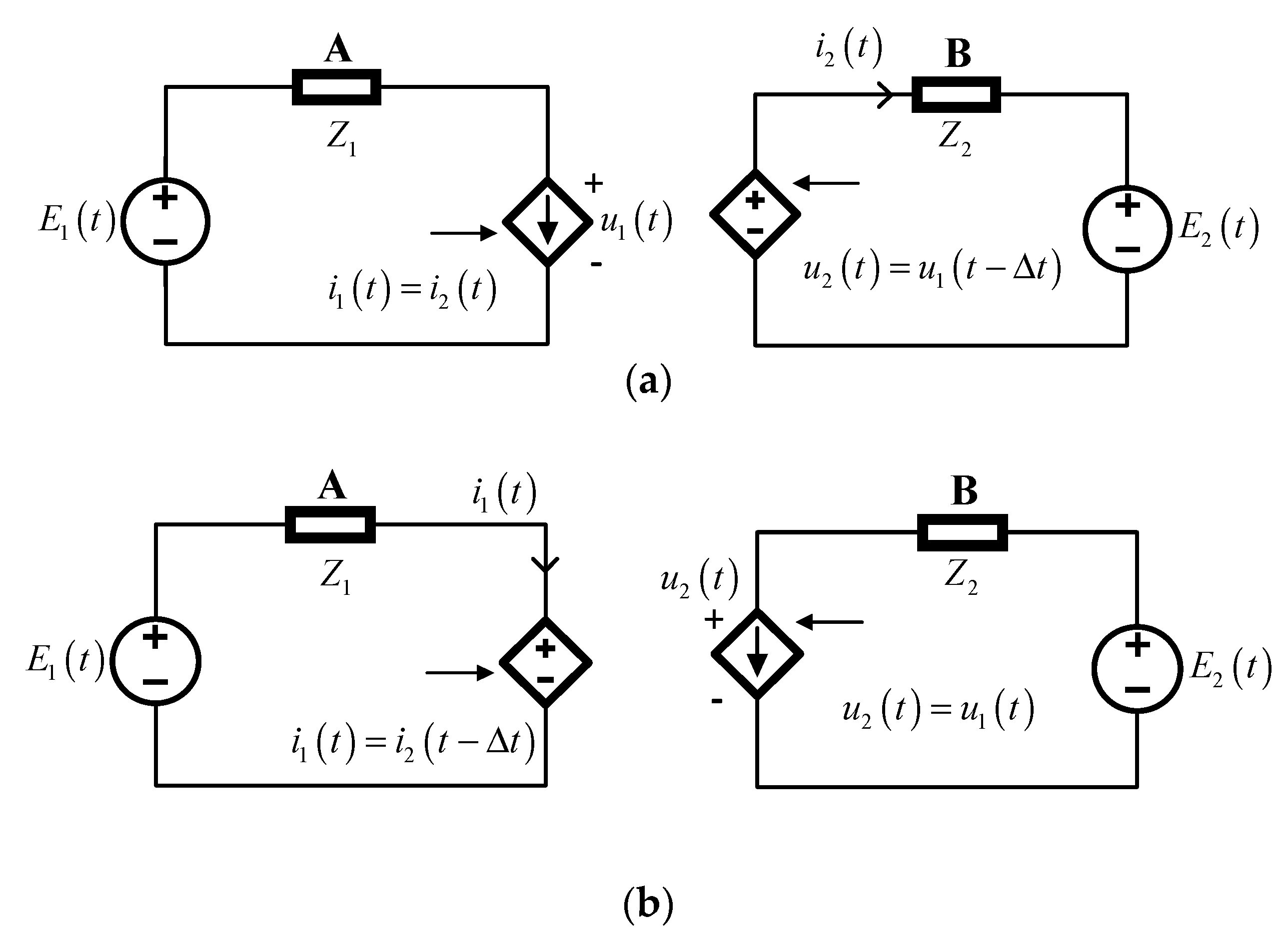
3.3. System-Decoupling Scheme and Improvement of Short-Line (Inductance)-Decoupling Method

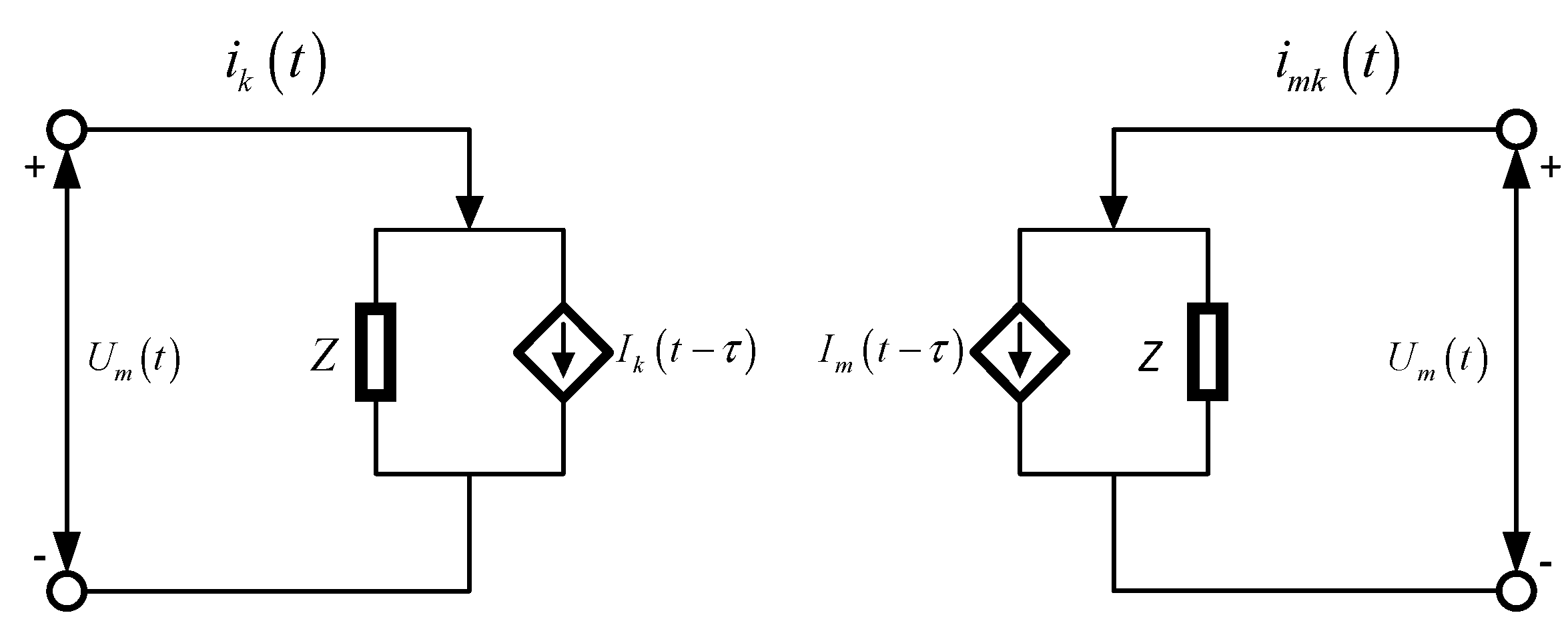
The decoupling of a long-distance transmission line is based on the characteristics of the line itself, so there is no numerical instability problem, and only the voltage and current signals at the opposite end need to be exchanged at both ends of the decoupling side, with small signal transmission. In addition, the influence of the time delay can be improved by combining the long-distance-transmission-line-decoupling method with SSN node splitting method [23]. However, the number of long-distance transmission lines in the model limits the use of this method.

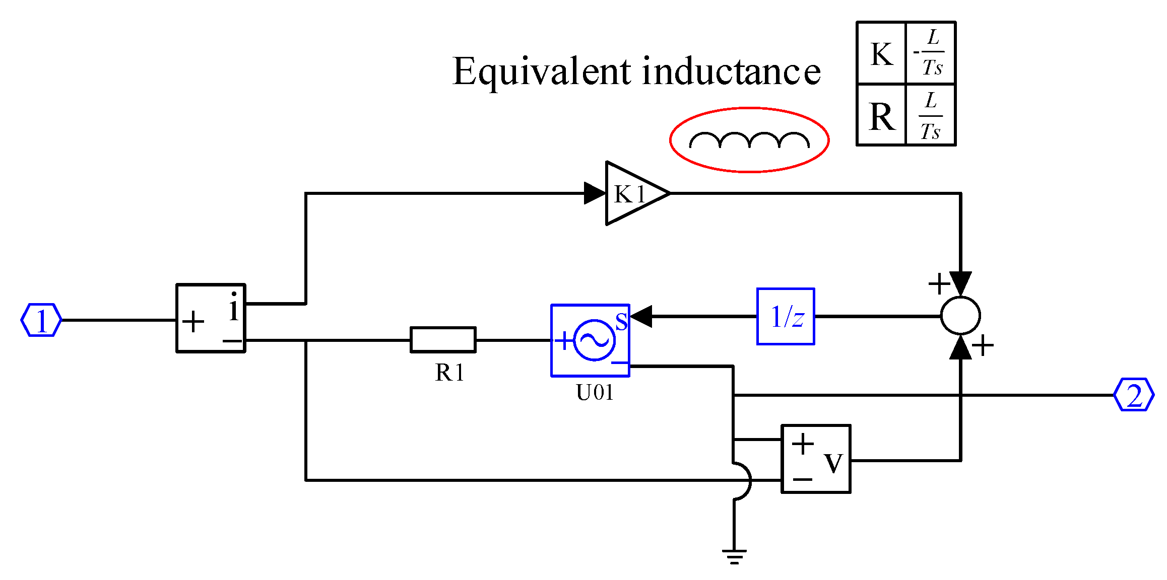
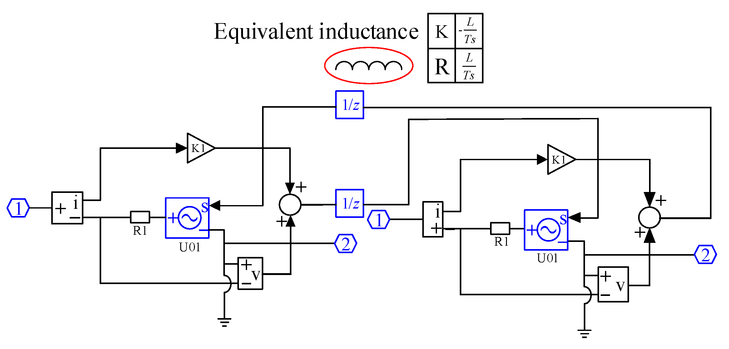
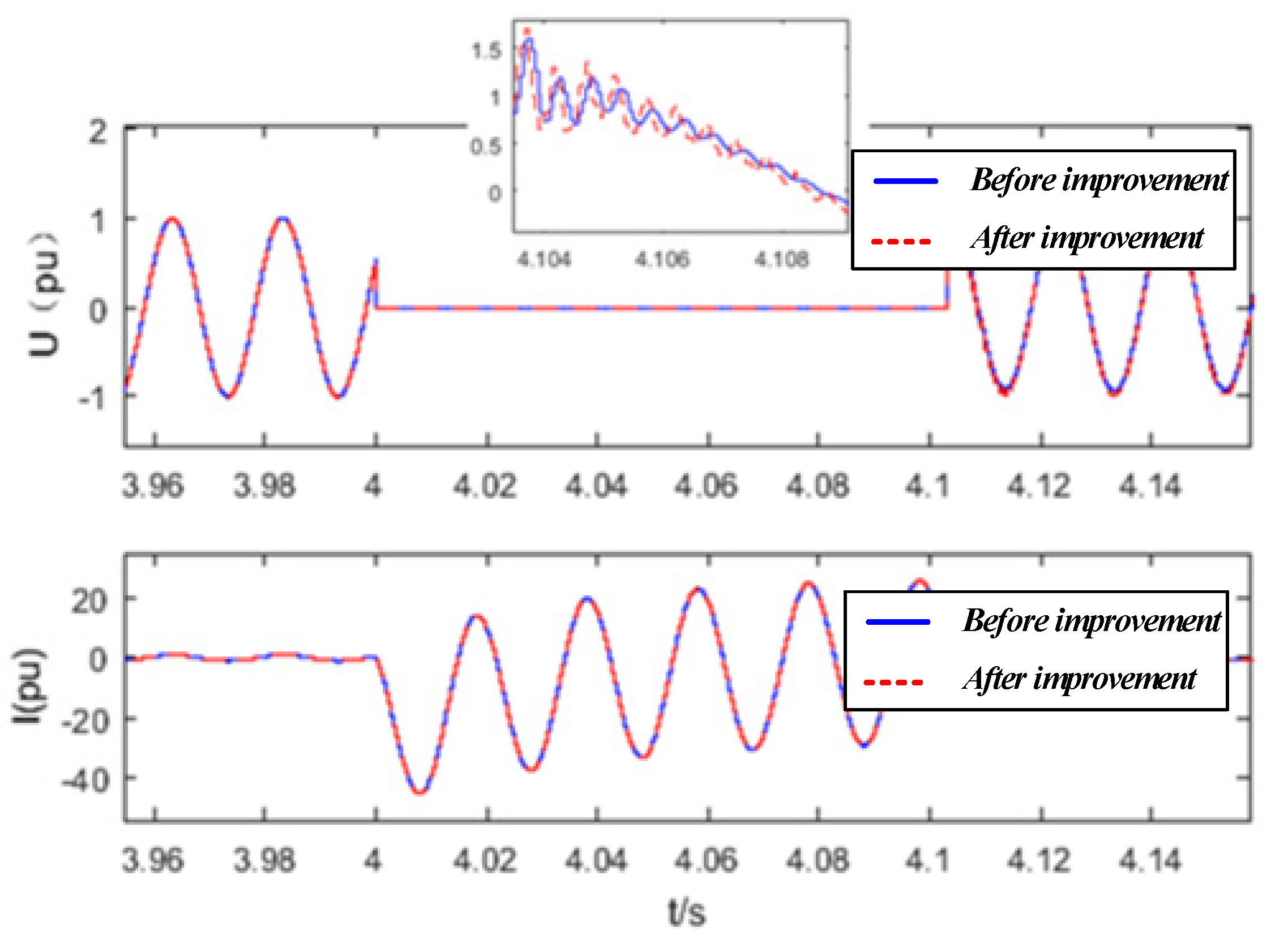
Short-line (inductance) decoupling is a relatively simple but widely applicable decoupling method. In practical application, the short line (the actual length is less than the transmission distance of a single step of the traveling wave) is usually replaced by a section of inductance. Due to the connection mode on the Y side of the transformer, it is also an option to extract the transformer inductance for decoupling. However, because this interface is modeled based on the trapezoidal-integration method, when the circuit breaker acts on the network, the trapezoidal-integration method will cause the abnormal oscillation (numerical oscillation) of the non-state variables. At present, the damping method is commonly used in engineering. In fact, mixing the trapezoidal-integration algorithm with the Euler method can also produce the same effect as the damping method [24,25].

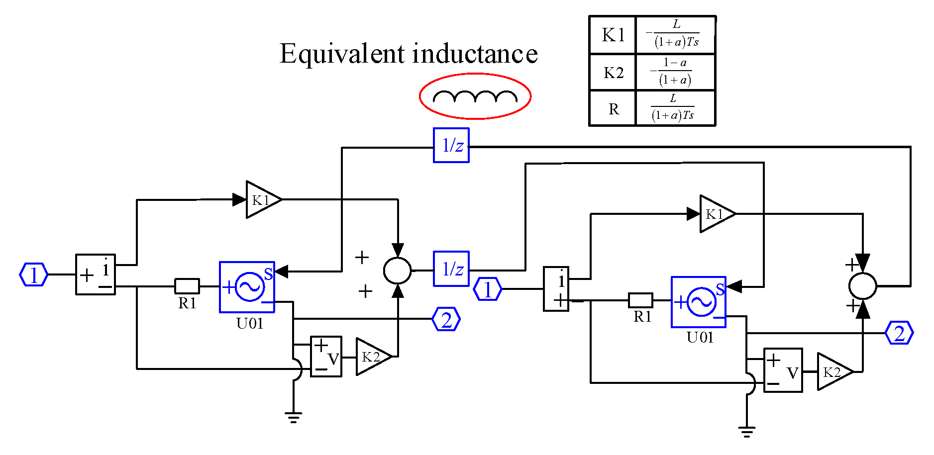
The discrete equation of inductance can be obtained by the backward Euler method

$$i_{km}(t)=\frac{\Delta t}{L}{(u_k-u_m)}_t+i_{km}(t-\Delta t)$$

(24)

If the proportion of the backward Euler method is a, and the proportion of trapezoidal-integration method is (1 − a), the mixed algorithm is as follows in Formula (25):

$$i_{km}(t)=\frac{(1+a)}{R_1}{(u_k-u_m)}_t+\frac{(1-a)}{R_1}{(u_k-u_m)}_{t-\Delta t}+i_{km}(t-\Delta t)$$

(25)

Figure 6 shows the improved interface algorithm. In this way, it is equivalent to the parallel a conductance of which the capacity is $a∆t/2L$ of the inductance, which shows the equivalence between the mixing of the backward Euler method and trapezoidal-integration method and the damping method.

3.4. Co-Simulation Platform-Segmentation Method

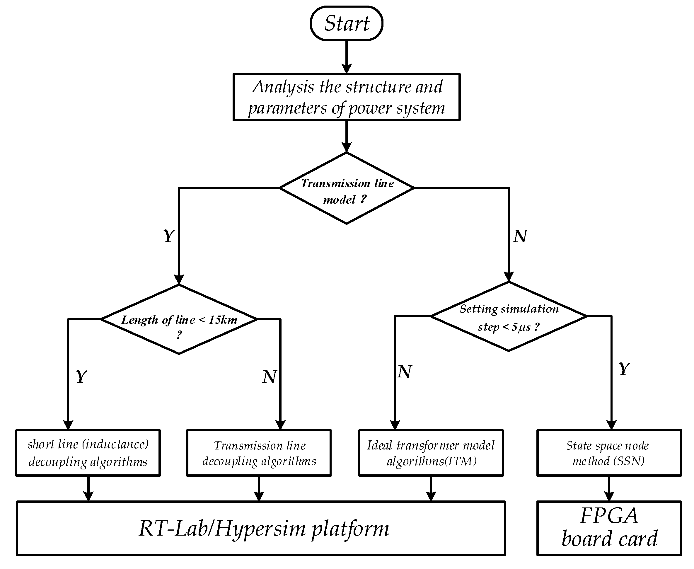
According to the analysis of four interface algorithms in Section 2, this paper uses the chosen criterion in this section as the rule of the proposed co-simulation platform.

This paper divides the whole system into two parts: one for the transmission line and one for the substation.

In comparison with the principle of the short-line decoupling algorithm, the minimum decoupling distributed-parameter-line length of the transmission-line-interface algorithm is 15 km [14,26]. Hence, this paper sets 15 km as the chosen criterion by which to divide the two types of line-interface algorithms. If the line length is less than 15km, then the interface algorithm chooses the short-line interface algorithm; if not, then the transmission-line algorithm will be chosen in the line-decoupling part.

The ideal-transformer-model method is widely used in engineering. It has the advantages of a simple structure, high operation accuracy and convenient improvement, but it has weak numerical stability. With the improvement of the system complexity, the operation scale becomes more and more complex. With regard to parallel operation, because the coupling signal needs to introduce an additional step delay, the introduction of the delay will not only lead to phase error but also amplitude error of the AC system, which must be improved by the compensation algorithm. At present, the widely used methods include interpolation prediction, the dq-transformation method and the impedance-matching method. The first two compensation methods are widely used in MMC model segmentation [16,27], but when there are sudden variables in the joint solution signal, the performance of the transient characteristics is not ideal. The impedance-matching method can better solve the problem of numerical instability, but with the increase in system complexity, the implementation of impedance matching will be more difficult. One study quickly decoupled the bridge-arm voltage and sub mode through the substitution theorem, so that the joint solution signal changed from a sudden variable to a continuous variable [28,29]. On this basis, interpolation prediction is used to better improve the transient characteristics.

When using the state-space-node (SSN) method for model-segmentation calculation, its main advantages are that there is no numerical instability problem, but there is good network flexibility and network segmentation can be carried out at any node. However, when using the SSN algorithm for model-segmentation calculation, each simulation step needs not only to transmit voltage and current signals, but also to calculate the Thevenin equivalent impedance of the segmented subsystem in real time and carry out real-time matching. This interface algorithm has a large amount of communication. Therefore, the SSN algorithm is very effective where there are many electronic switching devices, but overuse will lead to the communication time being greater than the time saved by model segmentation, so the SSN algorithm should be used appropriately.

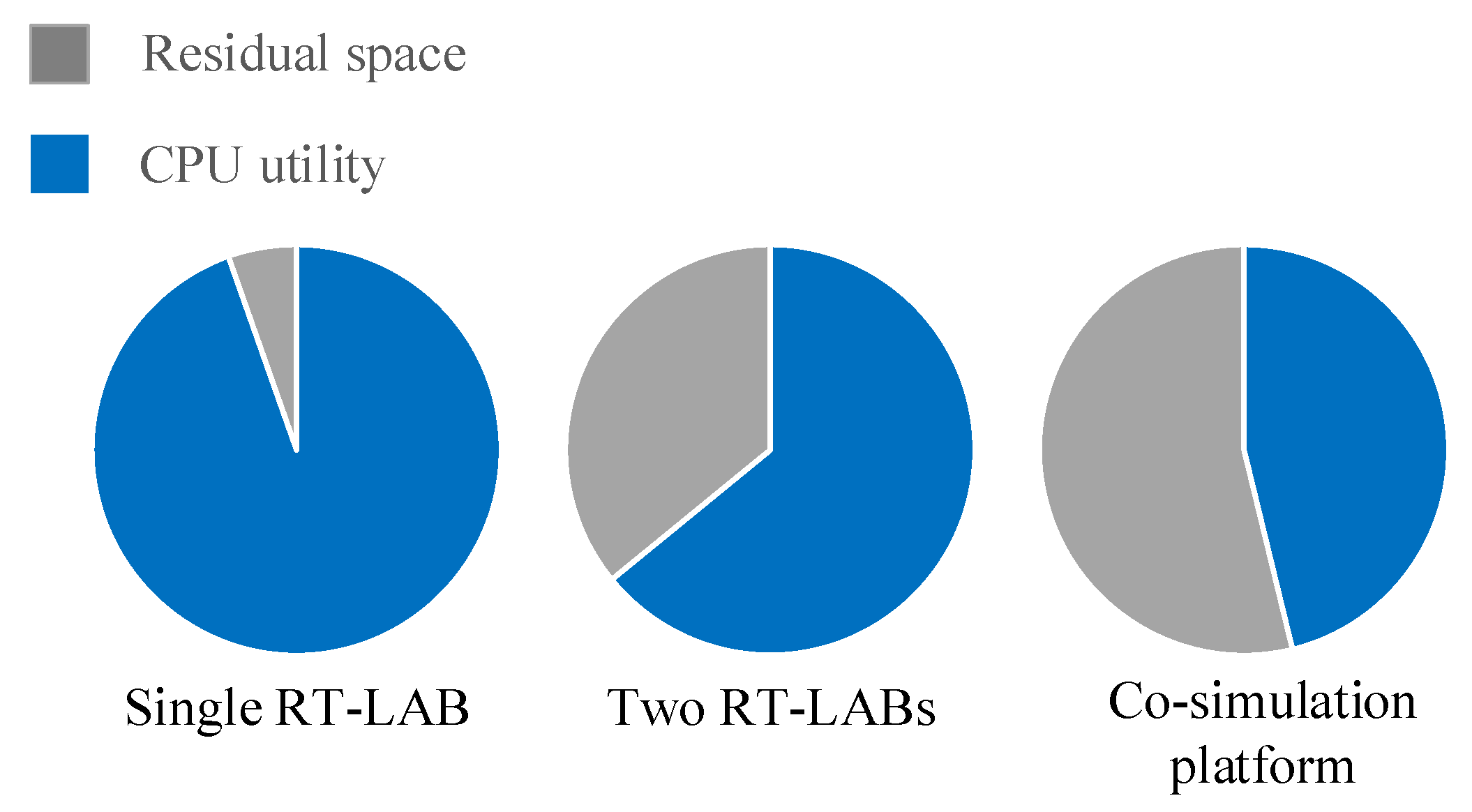
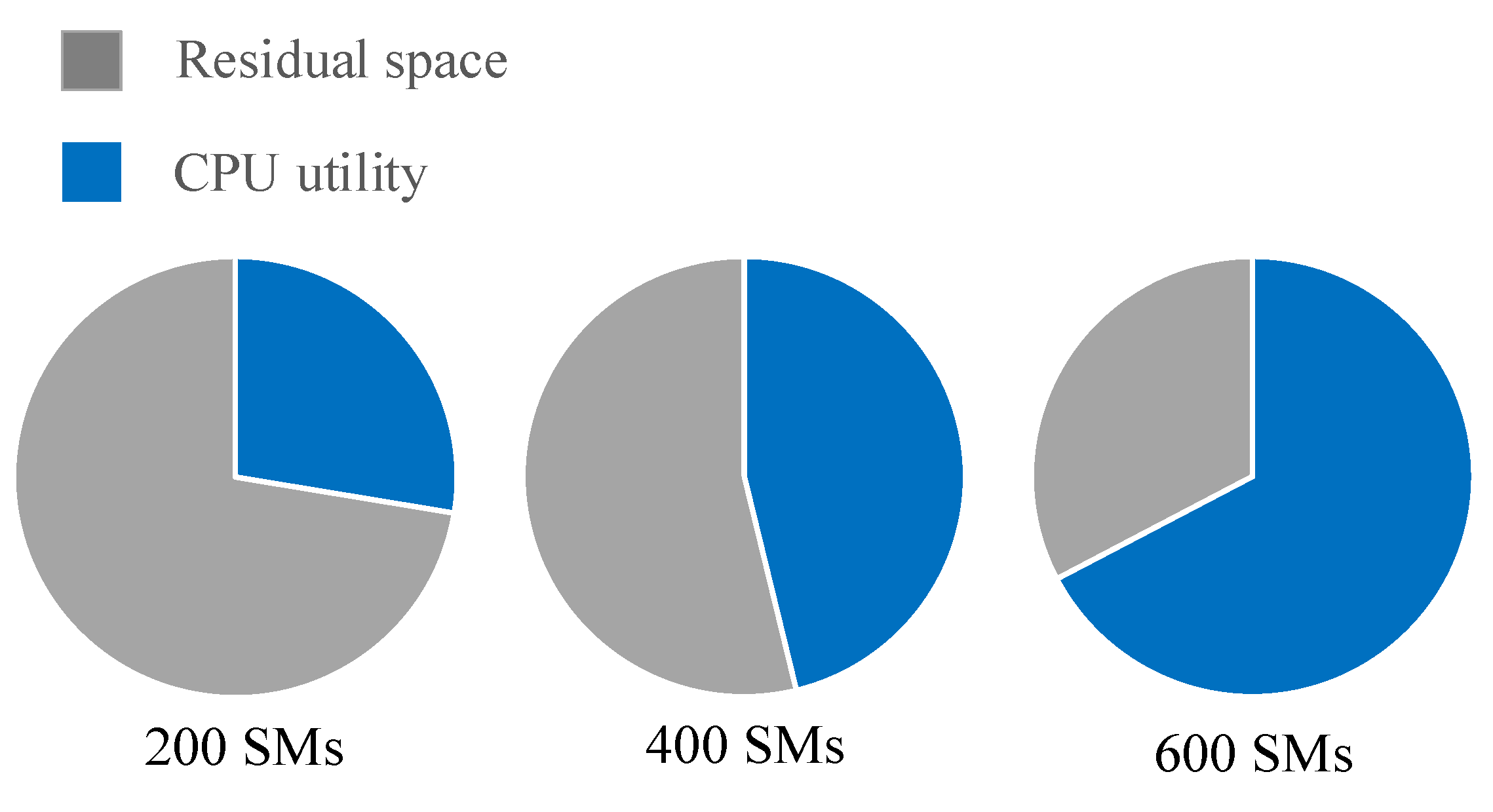
Hence, when choosing an interface algorithm in the substation part, according to the principle of increasing simulation efficiency, this paper set the simulation step time as the chosen criterion between the ideal-transformer-model algorithm and the SSN algorithm. The value of the simulation step time is $5\mathsf{\mu }s$ because the minimum simulation of RT-lab is $1\mathsf{\mu }s$, and simulation step time of $5\mathsf{\mu }s$ will introduce some errors to the platform.

In summary, the flowchart of the proposed co-simulation platform is shown in Figure 7.

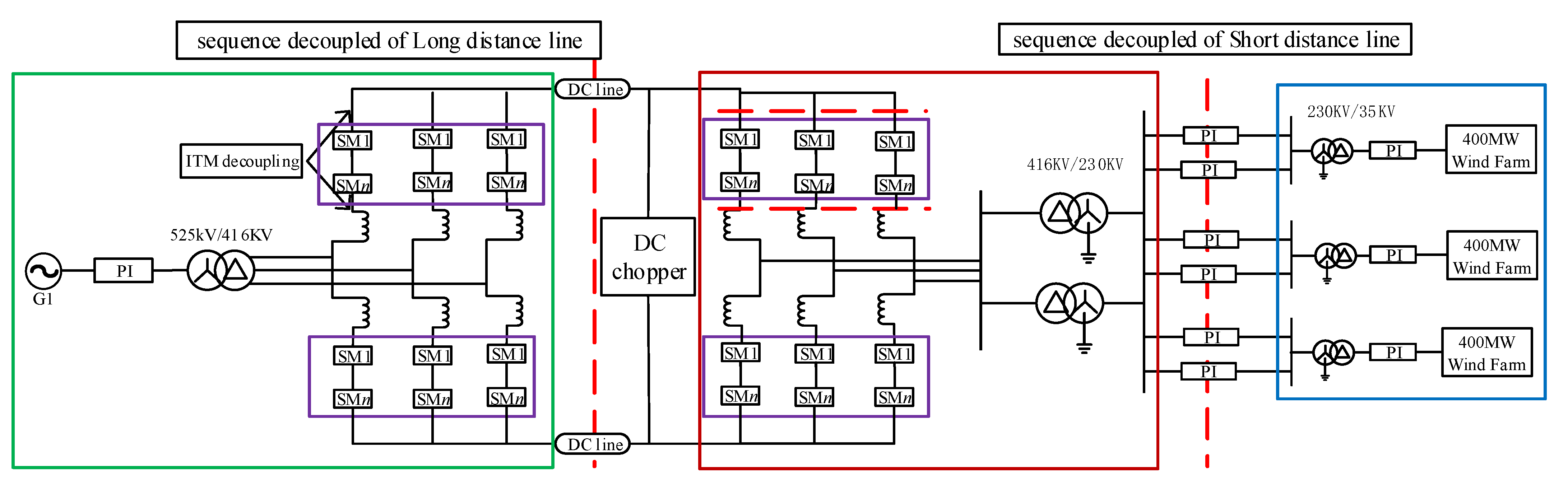
The fan is decoupled at different points through the flexible direct-delivery dual-platform-simulation model as an example. The decoupling method is shown in Figure 8. The large-scale system is decoupled at the short line between the offshore booster station and the booster station at the wind farm gathering point. The green form line is the Hypersim platform and the blue and red forms are the RT-lab co-simulation platforms. Both of the converter stations are decoupled at the DC line through long-line decoupling. The sub-module of the MMC bridge arm in the purple form is decoupled from the valve side through the ideal-transformer-model method. Here, the joint solution quantities are the bridge-arm current and the bridge-arm voltage. Since neither of them is a sudden-change quantity, interpolation prediction can better compensate for the delay. The AC/DC system is calculated in the CPU and the sub-module is calculated in the FPGA [6,29,30,31]. Due to the large number of power electronic devices of fans in the wind farm, the order is reduced through SSN decoupling in order to reduce the number of switches in the unit system and accelerate the operation.

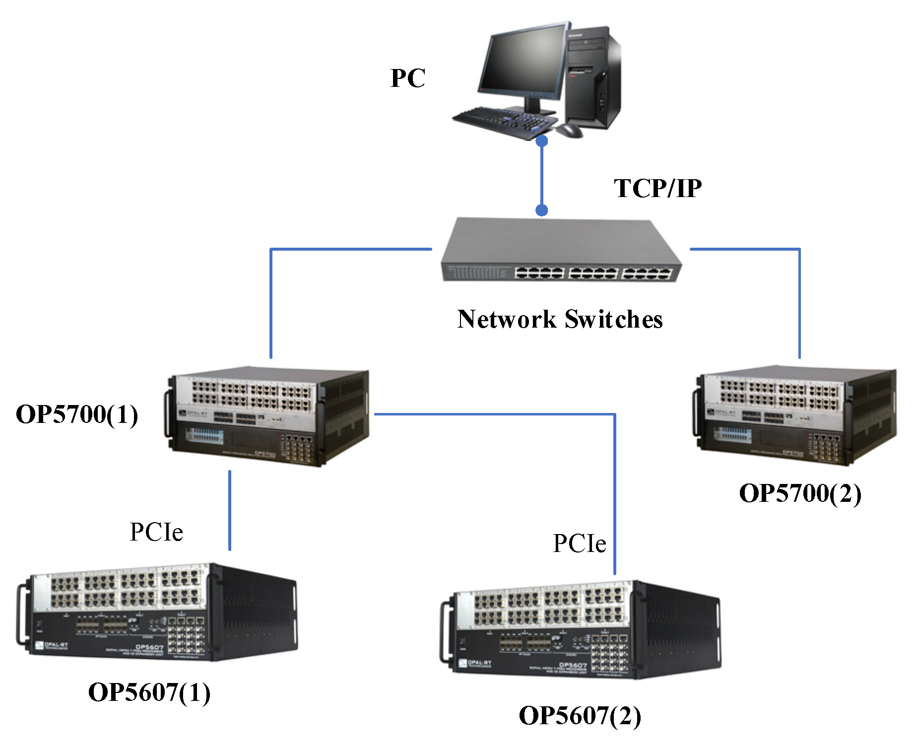
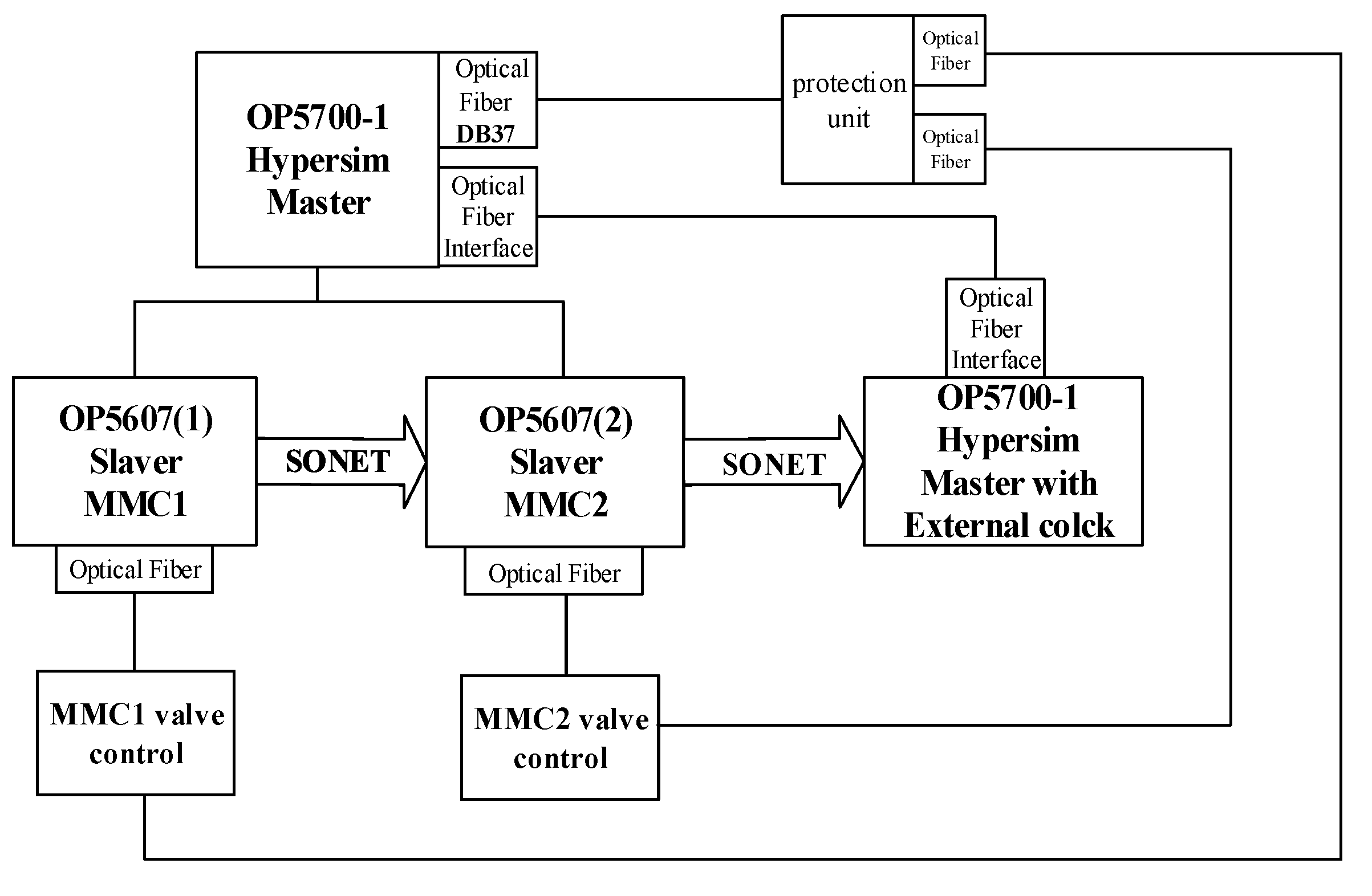
An unnecessary delay in co-simulation will mainly affect two aspects. On the one hand, an unnecessary delay will affect the stability of interface; on the other hand, a data delay will lead to an adverse impact on the control and protection [30] Therefore, clock synchronization and data interaction play important roles in the co-simulation platform. In order to solve the delay problem, an optical fiber using Aurora communication protocol, which is a scalable lightweight link-layer protocol for moving data between point-to-point serials, is adopted between OP5607 and OP5700 in the co-simulation platform. [31] The signal-transmission time is equal to a communication step which uses an FPGA cycle (50 μs). The simulation-connection-diagram flowchart is shown in Figure 9.

The proposed co-simulation model of a flexible DC-transmission system based on Hypersim mainly adopts three interface technologies: standard PCIe interface technology, high-speed optical-fiber-communication technology based on Aurora protocol, and low-speed optical-fiber-communication technology based on 60044-8 protocol. Among the rest, standard PCIe interface technology is used for the Hypersim inner protocol. According to the principle of Hypersim, the optical-fiber signal of the OP5607 adopts the Aurora 8B10B protocol, and the communication cycle is 50 μs (Hypersim calculation step). Hence, the FPGA cycle chooses 50 μs as a communication step in order to adapt to the Hypersim, and the signal-transmission time is equal to a communication step which also uses an FPGA cycle (50 μs). The optical fiber uses communication synchronization between platforms and each platform is defined as master and slave. The slave side obtains the system clock from the master side to keep the signal synchronized. The DB37 and optical-fiber communications are used between the FPGA and the pole-control modular, and the optical-fiber communication is used between the FPGA and the valve control. All of the communication cycles are set to one step (50 μs).

4. Simulation Verification

4.1. Simulation Comparison of Improved Short-Line (Inductance) Decoupling

In order to test the improved interface characteristics, the model shown in Figure 10 is adopted, and the decoupling points are shown in the figure. The improved interface model is compared with the original model under steady-state and transient conditions, respectively. The figure shows the A-phase voltage and current at the 35 kV bus side of the model in a steady state, while Figure 11 and Figure 12 show the three-phase grounding short-circuit fault at the secondary side of the 230 kV/35 kV transformer, and the waveform of the A-phase voltage and current at the 35 kV bus.

The blue line in the figure shows the waveform using the origin-coupling algorithm, and the red dotted portion represents the proposed short-line decoupling algorithm. It can be obtained from the steady-state and transient voltage and current waveforms. The improved decoupling mode is consistent with the amplitude and frequency before the improvement, and the waveform has no large distortion. In order to visually reflect it, it will be described later.

In order to prove the effect of the proposed improved decoupling method, FFT is used to analyze the steady- and transient-state harmonic-distortion rates (THD) of A-phase waveforms before and after the improvement.

The harmonic-distortion rate is a performance parameter that characterizes the distortion degree of a waveform relative to a sine wave in electrical engineering, abbreviated as THD. It is defined as the ratio of the root mean square value of all harmonic content to the root mean square value of the fundamental wave, expressed as a percentage [32].

The calculation of THD is shown as Formula (26)

$$THD=\sqrt{{\displaystyle \sum _{n=2}^H{\left(\frac{G_n}{G_1}\right)}^2}}$$

(26)

H is defined as the limited order, G_n represents the effective values of all the harmonic components, and G₁ represents the effective values of the fundamental wave.

Table 1. THD comparison of A-phase steady-state voltage and current.

THD	Without Interface/%	Before Improvement/%	After Improvement/%
Ua	1.54	1.76	1.68
Ia	2.34	2.46	2.41

and

Table 2. THD comparison of A-phase transient-state voltage and current.

THD	Without Interface/%	Before Improvement/%	After Improvement/%
Ua	3.04	3.21	3.14
Ia	3.97	4.10	3.99

shows the THD of A-phase waveforms before and after the improvement. From the table we can see that both the origin-decoupling method and the improved method are similar to the THD of a waveform without an interface, and the THD rate after the improvement is lower than the original model and before improvement.

4.2. Large Scale System Decoupling Simulation Test

In order to test the capacity of the proposed co-simulation platform, we have built the wind-power-based, flexible direct-transmission dual-platform-simulation model, which is shown in Figure 7, by using the proposed platform. In Figure 8, the capacity of converter station is 1100 MVA, each bridge arm has 400 sub-models, and the sub-mode rated voltage is 2000 V. DC voltage is ±400 kV.

4.2.1. Steady State Verification

When the wind farm is in full power and in steady-state operation, Figure 13, Figure 14, Figure 15, Figure 16, Figure 17, Figure 18 and Figure 19 show the voltage and current waveforms at the network side of the road-station system, the mmc1 valve side, and the DC side, and the power waveforms of the road station in the steady-state. In order to verify the feasibility, the THD comparison of the steady-state voltage and current are shown in

Table 3. THD comparison of steady-state voltage and current.

THD	Without Interface/%	Before Improvement/%	After Improvement/%
Ua	0.59	0.71	0.64
Ub	0.61	0.78	0.67
Uc	0.65	0.85	0.80
Ia	1.30	1.98	1.25
Ib	1.44	1.77	1.53
Ic	1.87	2.24	1.98

.

4.2.2. Transient-State Verification

A three-phase short-circuit grounding fault is applied to the network side of a 500 kV system, and the fault duration is 100 ms. In the case of a fault, the active power is rapidly reduced to 0. When the DC voltage reaches the input limit of energy-dissipation resistance, the energy-dissipation resistance is delayed to input, and the DC voltage will not rise again. After the fault is removed, the DC voltage drops rapidly and reaches the limit of energy-dissipation resistance, at which point the energy-dissipation resistance is delayed to exit. Figure 20, Figure 21, Figure 22, Figure 23, Figure 24 and Figure 25 show the voltage and current waveforms at the network side, mmc1 side, valve side and DC side of the road-station system respectively.

All the figures in Section 4.2 are shown as the simulation results of key points in the proposed platform, and the waveforms are conformed to the rated data.

Similarly, FFT is used to analyze the harmonic-distortion rate (THD) of three-phase waveforms before and after the improvement [24,31].

In summary, the simulation results prove the following two aspects:

• From the figure we can see that all the values of the simulation results (including voltage, current and power) are conformed to recording data of the rated system.
• It can be seen from Table 3 and

  Table 4. THD comparison of transient voltage and current.

  THD	Without Interface/%	Before Improvement/%	After Improvement/%
  Ua	1.84	1.91	1.80
  Ub	2.05	2.21	2.08
  Uc	1.94	2.32	2.08
  Ia	3.26	3.47	3.65
  Ib	2.88	3.28	3.01
  Ic	3.31	3.92	3.55

  that the harmonic-distortion rate after using the improvement interface in the proposed co-simulation platform is lower than that before the improvement, and both two methods are similar to the actual system without the interface, which proves the effectiveness of the improved interface.

4.3. Model-Resource-Occupancy Test

In order to test the resource-occupation rate of the improvement interface algorithm and the co-simulation platform proposed in this paper, the simulation model in Figure 7 is simulated and tested in MATLAB/Simulink based on a single RT-lab, two RT-labs, and the hardware architecture shown in Figure 5. The parameter of the apparatus is shown in

Table 5. Parameter of apparatus.

Items	Core Data
OP 5700	Intel® XeonE5-16 core * 2–2.3 GHz
PC (CPU)	Intel® Core i5-10400 CPU @ 2.90 GHz
FPGA	Xilinx®Virtex®7-485T

. In this section we will test the resource occupancy in two parts.

4.3.1. Occupancy of Improvement Algorithm

In order to test the resource-occupation rate of the improvement interface algorithm, we change the capacity of the wind turbine in Figure 7. The resource-occupation rate is compared with the origin and improvement algorithms in different capacities of the wind turbine, and the CPU occupation is shown in

Table 6. CPU occupancy of different wind-turbine capacities.

Capacity of Wind Turbine/MW	CPU Occupancy/%
	Before Improvement	After Improvement
200	34.1	30.3
400	45.7	41.5
600	59.4	52.6

.

From Table 6 we found that with the increase in capacity, the CPU occupancy of the two algorithms maintain an upward trend. Meanwhile, it also can be determined that the improvement algorithm has a lower CPU occupancy than the origin algorithm in the same type of platform, which proves the low resource-utilization rate of the improvement interface algorithm.

4.3.2. Occupancy of Improvement Algorithm

Based on the proposed co-simulation platform, CPU1 and CPU2 are the CPU occupancies of OP5700 (1) and OP5700 (2), CPU3 is the FPGA occupancy of OP5607, and CPU4 is the CPU occupancy of the Hypersim tester (PC). The CPU occupancy of the above model in the real-time simulation process is tested and the results are shown in

Table 7. CPU occupancy of different simulation structures.

Item	Total Occupancy/%	Occupancy/%
		CPU1	CPU2	CPU3	CPU4
Single RT-lab	94.6	94.6	-	-	-
Two RT-lab	57.4	41.5	64.1	-	-
co-simulation platform	30.8	41.5	29.1	46.2	18.4

.

Figure 26 shows the occupancy ratio of the maximum CPU utilization in each hardware by different simulation-platform strategies. According to the description of the RL-LAB hardware conditions, when the CPU utility exceeds 80%, the system will not run normally and the host computer will report error messages. The left pie chart shows that the CPU utility exceeds 80% in the current system by a single RT-lab, and during the simulation process an error occurred. Although the two RT-labs co-simulation platform has a lower CPU utility, the highest utility is over 60%. When using the presented co-simulation platform, the highest utility did not exceed 50%. As the system grows larger and larger, the residual space of the improved co-simulation platform is large enough to simulate.

In order to verify the extensibility of the proposed co-simulation platform, 200 SMs, 400 SMs and 600 SMs MMC-HVDC converter structures were built by the improved co-simulation platform for simulation testing. Figure 26 shows the highest CPU utility of each converter structure.

From Figure 27 we can see that with the increase in the number of SMs, the CPU utility has been enhanced to within the acceptable range. It proves that the improved interface algorithm has a strong expansion performance and is suitable for the construction of complicated models.

In conclusion, when a single RT-lab performs the simulation, with the continuous expansion of the system scale, the kernel-occupancy rate is high. When the system continues to expand, the CPU load rate will further expand, which will affect the accuracy and feasibility of the simulation. The CPU occupancy of the joint-simulation structure proposed in this paper is effectively controlled below 50%, leaving a sufficient threshold for the subsequent expansion of the simulation scale.

5. Conclusions

This paper has proposed a co-simulation-platform strategy based on the model-segmentation algorithm in order to simultaneously deal with the consideration of the data interactions of large- and small-step systems when building a hybrid system. The proposed method uses different decoupling algorithms for different topologies in order to decouple complex systems from multiple units, and each unit can run in an independent simulation platform (hardware or software).

An improved short-line decoupling algorithm is proposed and applied in a co-simulation platform that aims to suppress the transient oscillation that occurs due to harmonic suppression. A wind-power-based, flexible direct-transmission dual-platform-simulation model was built in cross-platform with RT-lab and Hypersim. The proposed simulation strategy can efficiently suppress the transient oscillation of the system and maintain high-speed communication. In particular, the simulation platform based on the proposed strategy has a strong expansibility for complex systems.

Based on the advantages and disadvantages of the above interface algorithm, the cross-platform joint-simulation model that was sent by the wind farm through flexible and direct transmission is understood and coupled, and the cross-platform simulation and model-decoupling-segmentation scheme proposed in this paper is verified to be feasible through the steady-state and transient experiments of the road station. However, it should be noted that the proposed interface algorithm still has room for improvement in the case of large disturbances, in order to improve the accuracy of the interface algorithm.

References

1. Faruque, M.D.O.; Strasser, T.; Lauss, G.; Jalili-Marandi, V.; Forsyth, P.; Dufour, C.; Dinavahi, V.; Monti, A.; Kotsampopoulos, P.; Martinez, J.A.; et al. Real-Time Simulation Technologies for Power Systems Design, Testing, and Analysis. IEEE Power Energy Technol. Syst. J. 2015, 2, 63–73. [Google Scholar] [CrossRef]
2. Ren, W.; Sloderbeck, M.; Steurer, M.; Dinavahi, V.; Noda, T.; Filizadeh, S.; Chevrefils, A.R.; Matar, M.; Iravani, R.; Dufour, C.; et al. Interfacing Issues in Real-Time Digital Simulators. IEEE Trans. Power Deliv. 2011, 26, 1221–1230. [Google Scholar] [CrossRef]
3. Tian, F.; Zhou, X. Partition and Parallel Method for Digital Electromagnetic Transient Simulation of AC/DC Power System. Proc. CSEE 2011, 31, 1–7. [Google Scholar] [CrossRef]
4. Lin, J.; Yan, Y.; Liu, T.; Zheng, W. Review on External System Equivalent Method for Electromagnetic Transient Simulation of Power Systems. Autom. Electr. Power Syst. 2012, 36, 108–115. [Google Scholar] [CrossRef]
5. Dufour, C.; Bélanger, J. On the Use of Real-Time Simulation Technology in Smart Grid Research and Development. IEEE Trans. Ind. Appl. 2014, 50, 3963–3970. [Google Scholar] [CrossRef]
6. Wang, Y.; Liu, C.; Gengyin, L.I. FPGA-based Real-time Modeling of Modular Multilevel Converters and Hardware-in-the-loop Simulation. Proc. CSEE 2018, 38, 3912–3920. [Google Scholar] [CrossRef]
7. Teninge, A.; Besanger, Y.; Colas, F.; Fakham, H.; Guillaud, X. Real-time simulation of a medium scale distribution network: Decoupling method for multi-CPU computation. In Proceedings of the 2012 Complexity in Engineering (COMPENG), Aachen, Germany, 11–13 June 2012; pp. 1–6. [Google Scholar] [CrossRef]
8. Venkatraman, R.; Khaitan, S.K.; Ajjarapu, V. Dynamic Co-Simulation Methods for Combined Transmission-Distribution System with Integration Time Step Impact on Convergence. IEEE Trans. Power Syst. 2019, 34, 1171–1181. [Google Scholar] [CrossRef]
9. Sadnan, R.; Krishnamoorthy, G.; Dubey, A. Transmission and Distribution (T&D) Quasi-Static Co-Simulation: Analysis and Comparison of T&D Coupling Strength. IEEE Access 2020, 8, 124007–124019. [Google Scholar] [CrossRef]
10. Hooshyar, H.; Vanfretti, L.; Dufour, C. Delay-free parallelization for real-time simulation of a large active distribution grid model. In Proceedings of the IECON 2016—42nd Annual Conference of the IEEE Industrial Electronics Society, Florence, Italy, 23–26 October 2016; pp. 6278–6284. [Google Scholar] [CrossRef] [Green Version]
11. Fei, L.; Huang, S.; Hao, Z.; Hao, Z.; Chen, Z.; Tan, Z.; Xu, Y. Model segmentation method for real-time simulation of DC power transmission system. Exp. Technol. Manag. 2018, 35, 139–143. [Google Scholar] [CrossRef]
12. Liu, T.; Yan, Y.P.; Jin, N. Interpolation Algorithm for Electromagnetic Transient Simulation Considering Multiple Switching Events. Proc. CSU-EPSA 2013, 6, 143–147. [Google Scholar]
13. Liu, S.; Wang, H.; Wang, H.; Wang, Z.; Sun, C.; Zhu, G.; Fu, X. Research on interface algorithm based on cross-platform joint simulation technology. Electr. Meas. Instrum. 2019, 56, 70–74. [Google Scholar] [CrossRef]
14. Hu, Y.; Zhang, P.; Fang, C.; Bao, H. Power Hardware-in-the-loop Simulation System Part One Characteristics of Interface Algorithms. Autom. Electr. Power Syst. 2013, 37, 36–41. [Google Scholar]
15. Qing, M.; Yalou, L.; Xiaoxin, Z.; Peng, Z.; Xing, Z. A parallel multi-rate electromagnetic transient simulation algorithm based on network division through transmission line. Autom. Electr. Power Syst. 2014, 38, 47–52. [Google Scholar]
16. Yang, X.; Sun, Q.; Du, Y.; Su, J. Performance Analysis of Power Hardware-in-Loop Simulation. Power Syst. Technol. 2019, 43, 251–262. [Google Scholar]
17. Zhang, H.; Hao, Z.; Chen, Z.; Wu, Y.; Xiao, Z.; Yuan, W. Modeling Method for Real Time Simulation of Modular Multilevel Converter. Autom. Electr. Power Syst. 2017, 41, 120–126. [Google Scholar]
18. Dufour, C.; Mahseredjian, J.; Bélanger, J. A combined state-space nodal method for the simulation of power system transients. In Proceedings of the 2011 IEEE Power and Energy Society General Meeting, Boston, MA, USA, 17–21 July 2011; pp. 928–935. [Google Scholar] [CrossRef]
19. Xin, Y.; Jiang, S.; Li, G.; Wang, L. Review on interface algorithms of power hardware-in-the-loop simulation for power systems. Autom. Electr. Power Syst. 2016, 40, 159–167. [Google Scholar] [CrossRef]
20. Wei, T.; Qiu, H.J.; Zou, Y.J. Application of SSN algorithm in large wind power system real-time simulation. Power Syst. Prot. Control 2014, 42, 98–103. [Google Scholar]
21. OPAL-RT Technologies. RT-LAB ver. 2019.2.3.176; OPAL-RT Technologies: Montreal, QC, Canada, 2019; Available online: https://www.opal-rt.com/zh-hans/ (accessed on 13 December 2021).
22. Baorong, Z.; Dazhong, F.; Snider, L.A.; Chen, J. The Fully Digital Real-Time Simulator—Hypersim. Autom. Electr. Power Syst. 2003, 19, 79–82. [Google Scholar]
23. Yang, M.; Zhang, Y.M.; Zhang, Z.Q.; Gu, Y.X. Summary of Research on Electromagnetic Transient Simulation Algorithm of Power System. Electrical Measurement and Instrumentation: 1–11. Available online: http://kns.cnki.net/kcms/detail/23.1202.TH.20210415.1530.008.html (accessed on 15 November 2021).
24. Li, P.; Wang, Z.; Wang, C.; Fu, X.; Song, Y. Design of Parallel Architecture for Multi-FPGA Based Real-time Simulator of Active Distribution Network. Autom. Electr. Power Syst. 2019, 43, 174–182. [Google Scholar] [CrossRef]
25. Li, W.; Jean, B. An equivalent circuit method for modelling and simulation of modular multilevel converter in real-time HIL test bench. In Proceedings of the 2017 IEEE Power & Energy Society General Meeting, Chicago, IL, USA, 16–20 July 2017; p. 1. [Google Scholar] [CrossRef]
26. Zhang, N.; Sun, J.J.; Cheng, C.; Cao, Z.; Pan, J.; Xu, B. Electromechanical electromagnetic transient hybrid simulation interface model based on high frequency equivalent impedance. Electr. Meas. Instrum. 2020, 57, 1–6. [Google Scholar]
27. Guo, R.; Zhao, Y.; Gao, W. Numerical calculation method of electromagnetic transient of high voltage transmission lines based on lock generalized backward difference method. Shaanxi Electr. Power 2019, 47, 82–86, 92. [Google Scholar]
28. Wang, W.; Zhu, J.; Wei, L.; Zou, Y. SSN-Based RT-LAB Simulation of MMC-HVDC System. South. Power Syst. Technol. 2015, 6, 22–27. [Google Scholar]
29. Saad, H.; Ould-Bachir, T.; Mahseredjian, J.; Dufour, C.; Dennetiere, S.; Nguefeu, S. Real-Time Simulation of MMCs Using CPU and FPGA. IEEE Trans. Power Electron. 2015, 30, 259–267. [Google Scholar] [CrossRef]
30. Chengshan, W.; Peng, L.; Bibin, H.; Liwei, W.; Fei, G. An Interpolation Algorithm for Time-Domain Simulation of Power Electronics Circuit Considering Multiple Switching Events. Trans. China Electrotech. Soc. 2010, 25, 83–88. [Google Scholar] [CrossRef]
31. 61912—Aurora Solution Center—Design Assistant. Available online: https://support.xilinx.com/s/article/61912?language (accessed on 10 December 2021).
32. Zhai, X.; Lin, C.; Gregoire, L.-A.; Wang, W.; Li, W.; Zhang, F.; Joos, G. Multi-rate real-time simulation of modular multilevel converter for HVDC grids application. In Proceedings of the IECON 2017—43rd Annual Conference of the IEEE Industrial Electronics Society, Beijing, China, 29 October–1 November 2017; pp. 1325–1330. [Google Scholar]
Figure 1. Nondestructive single-phase Distributed Parameters Line model.
Electronics 10 03185 g001
Figure 2. Equivalent mathematical model of inductance.
Electronics 10 03185 g002
Figure 3. Equivalent mathematical model of inductance decoupling.
Electronics 10 03185 g003
Figure 4. Ideal transformer model: (a) Voltage-type ideal transformer model; (b) Current-type ideal transformer model.
Electronics 10 03185 g004
Figure 5. Co-simulation of hardware architecture.
Electronics 10 03185 g005
Figure 6. Improved interface mathematical model.
Electronics 10 03185 g006
Figure 7. Flowchart of co-simulation platform segmentation method.
Electronics 10 03185 g007
Figure 8. Schematic diagram of system decoupling point.
Electronics 10 03185 g008
Figure 9. System connection diagram.
Electronics 10 03185 g009
Figure 10. Improved interface test model.
Electronics 10 03185 g010
Figure 11. Steady-state voltage and current waveform comparison.
Electronics 10 03185 g011
Figure 12. Transient voltage and current waveform comparison.
Electronics 10 03185 g012
Figure 13. Network-side voltage waveform of land system.
Electronics 10 03185 g013
Figure 14. Current waveform at the network side of land system.
Electronics 10 03185 g014
Figure 15. MMC1 valve-side voltage waveform.
Electronics 10 03185 g015
Figure 16. MMC1 valve-side current waveform.
Electronics 10 03185 g016
Figure 17. DC-side voltage waveform.
Electronics 10 03185 g017
Figure 18. DC-side current waveform.
Electronics 10 03185 g018
Figure 19. Land station power waveform.
Electronics 10 03185 g019
Figure 20. Network-side voltage waveform of land system.
Electronics 10 03185 g020
Figure 21. Current waveform at the network side of land system.
Electronics 10 03185 g021
Figure 22. MMC1 valve-side voltage waveform.
Electronics 10 03185 g022
Figure 23. MMC1 valve-side current waveform.
Electronics 10 03185 g023
Figure 24. DC-side voltage waveform.
Electronics 10 03185 g024
Figure 25. Land station power waveform.
Electronics 10 03185 g025
Figure 26. Highest CPU utility in each platform.
Electronics 10 03185 g026
Figure 27. Highest CPU utility in different MMC converter models.
Electronics 10 03185 g027