
Political-Optimizer-Based Energy-Management System for Microgrids

 ,
,  ,
,  ,
,  ,
,
Abstract
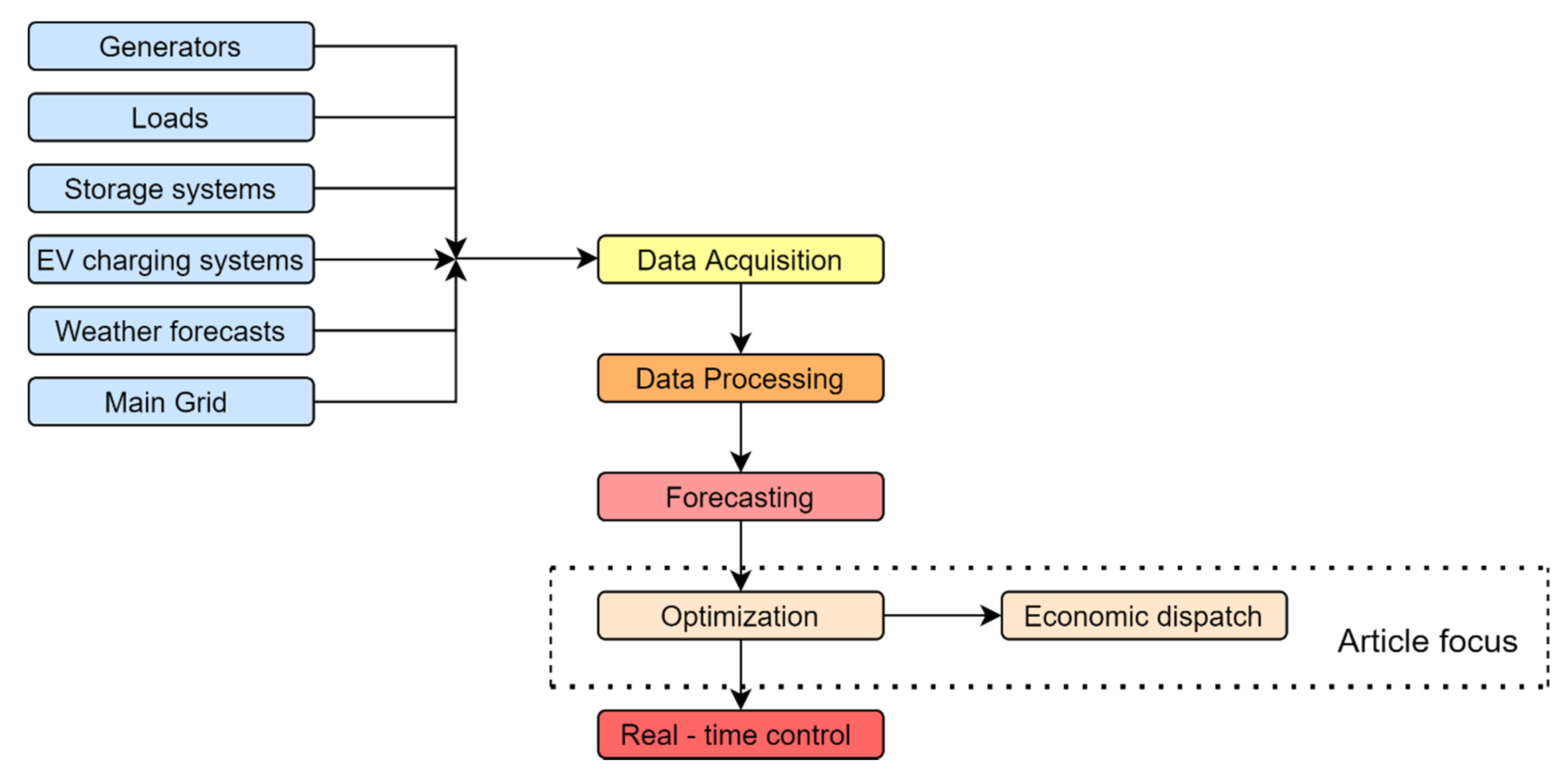
:1. Introduction
- The examples provided above used different optimization algorithms in order to carry out the ED or energy management in diverse microgrids. In fact, new optimization algorithms are always being developed and it is not clear which optimization algorithm would serve as the best for the EMSs of microgrids. The question is quite relevant given the rapid adoption and development of microgrids. In this regard, the contributions of this paper are summarized as follows:
- The investigation of two recently developed optimization algorithms for carrying out Optimal-Power-Flow (OPF) studies in electrical networks. This step is essential since it is important to test any new approach on a standard, well-known system before it is used for energy management in highly localized and diverse microgrids. The tested algorithms include the Political Optimizer (PO) and the Lichtenberg Algorithm (LA). The OPF studies were carried out by the cost minimization of the IEEE 30-bus system.
- The comparison of the performance of the newly developed approaches with existing conventional approaches. In this regard, a comprehensive comparison of the values of all the decision variables as a result of applying the PO and LA were compared with the results from applying the Particle Swarm Optimization (PSO) and Genetic Algorithm (GA). Furthermore, a small comparison of the results taken from the well-known literature was also made.
- The best performing optimization algorithm was then selected to carry out ED studies in a microgrid that consisted of numerous sources of energy such as Li-ion storage systems, fuel cells (FCs), solar PV panels, micro-hydro power plants and diesel generators (DGs). The LCOE of all the sources of energy were calculated and it was found to be minimized during the operation of the microgrid. The microgrid was connected and hourly grid prices were used in the study.
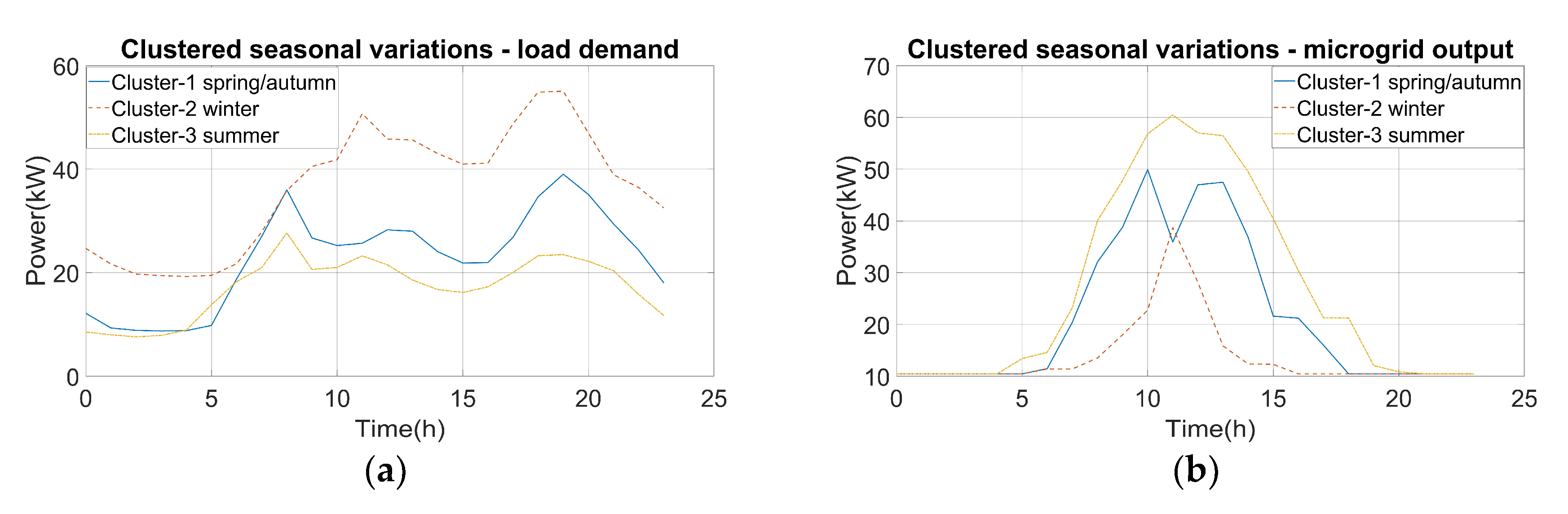
- Finally, in order to understand the cost implications year round, clustering was used to identify representative days of the year with which comparisons were made regarding the microgrid operation. The microgrid model was based on the existing elements present at Wroclaw University of Science and Technology.
- The novelty of the study comes from the fact that the Political Optimizer and the Lichtenberg Algorithm have not yet been used for OPF studies. Moreover, the study shows that the Political Optimizer is an effective option for an energy-management system of microgrids, which, to the best of our knowledge, has not yet been explored. The study presents an energy-management approach that analyzes the behavior of the microgrid and the LCOE cost for an entire year, which is valuable to microgrid planners in the region.
2. Investigated Optimization Algorithms
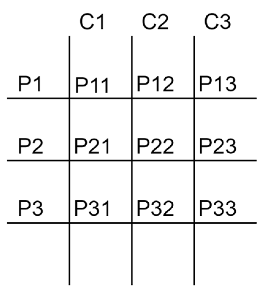
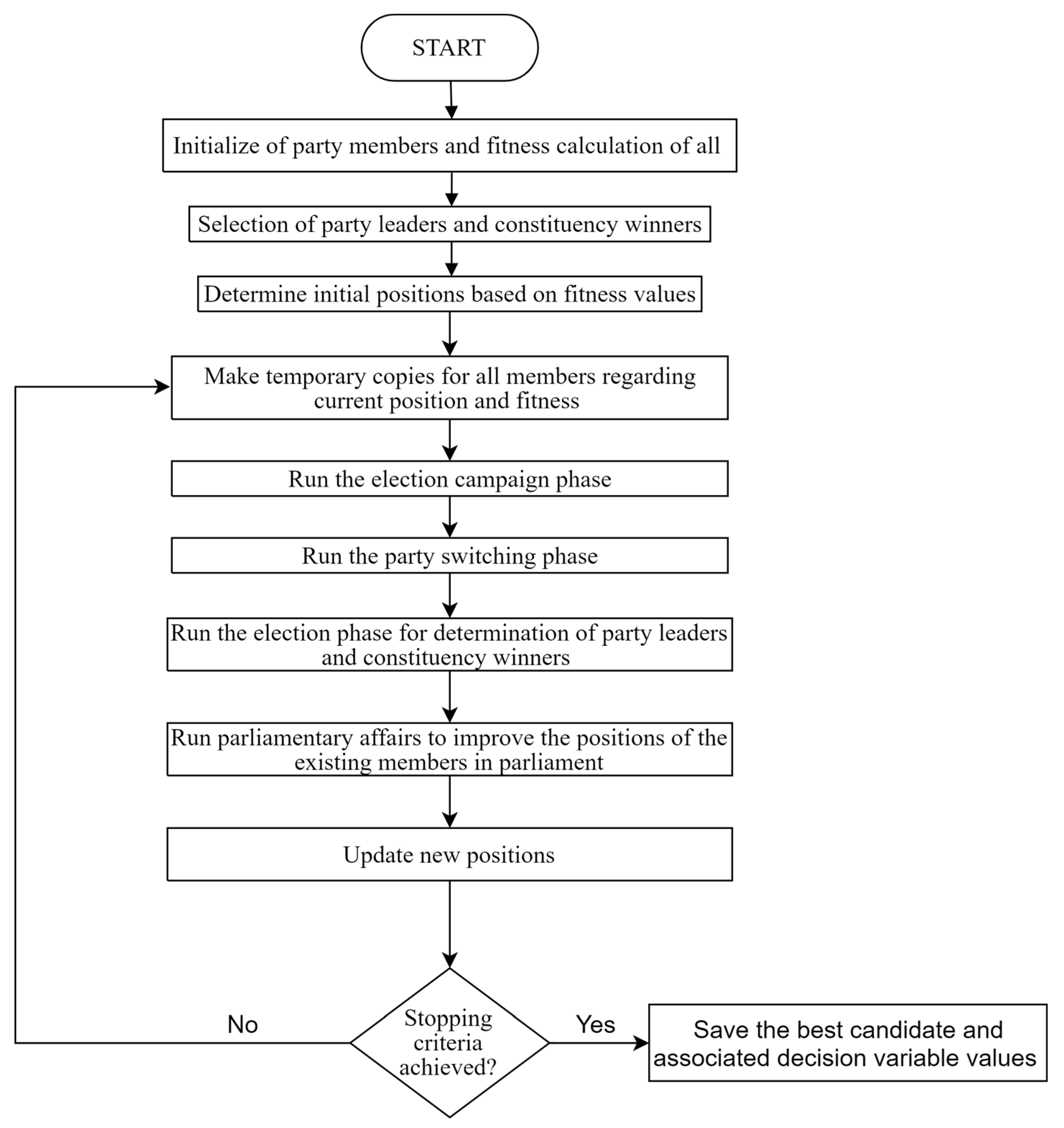
2.1. Political Optimizer
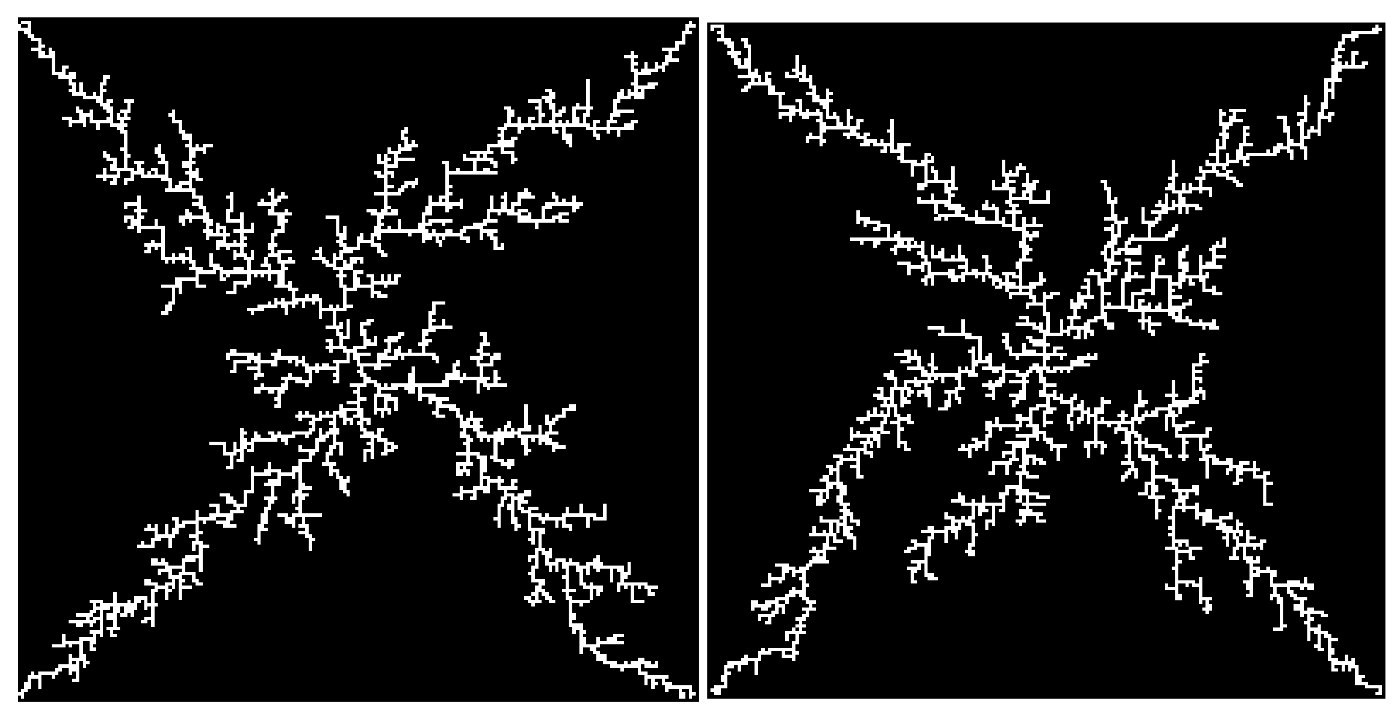
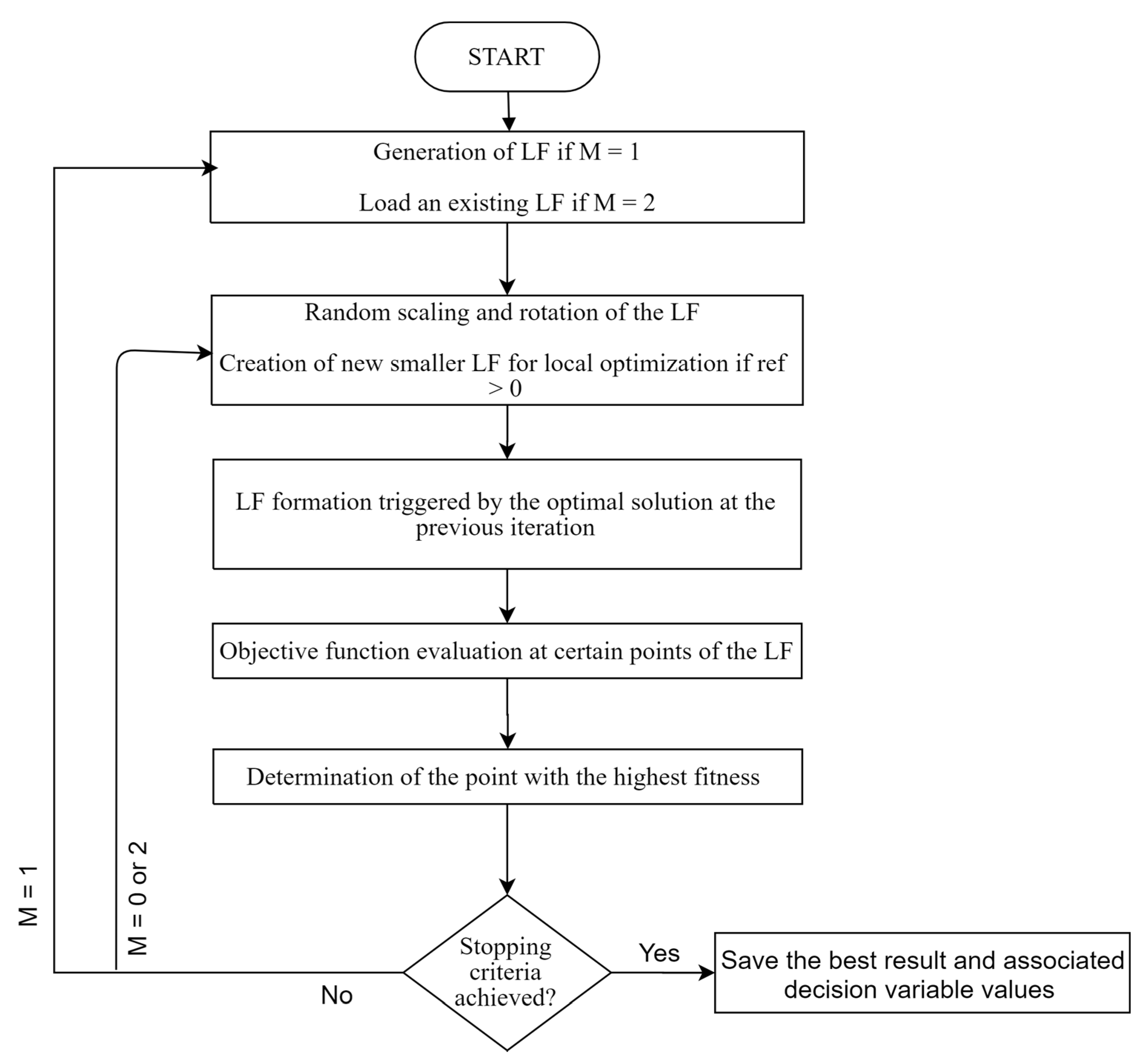
2.2. Lichtenberg Algorithm
2.3. Performance Evaluation of the Investigated Algorithms
3. Microgrid Layout, Mathematical Model and LCOE Calculations
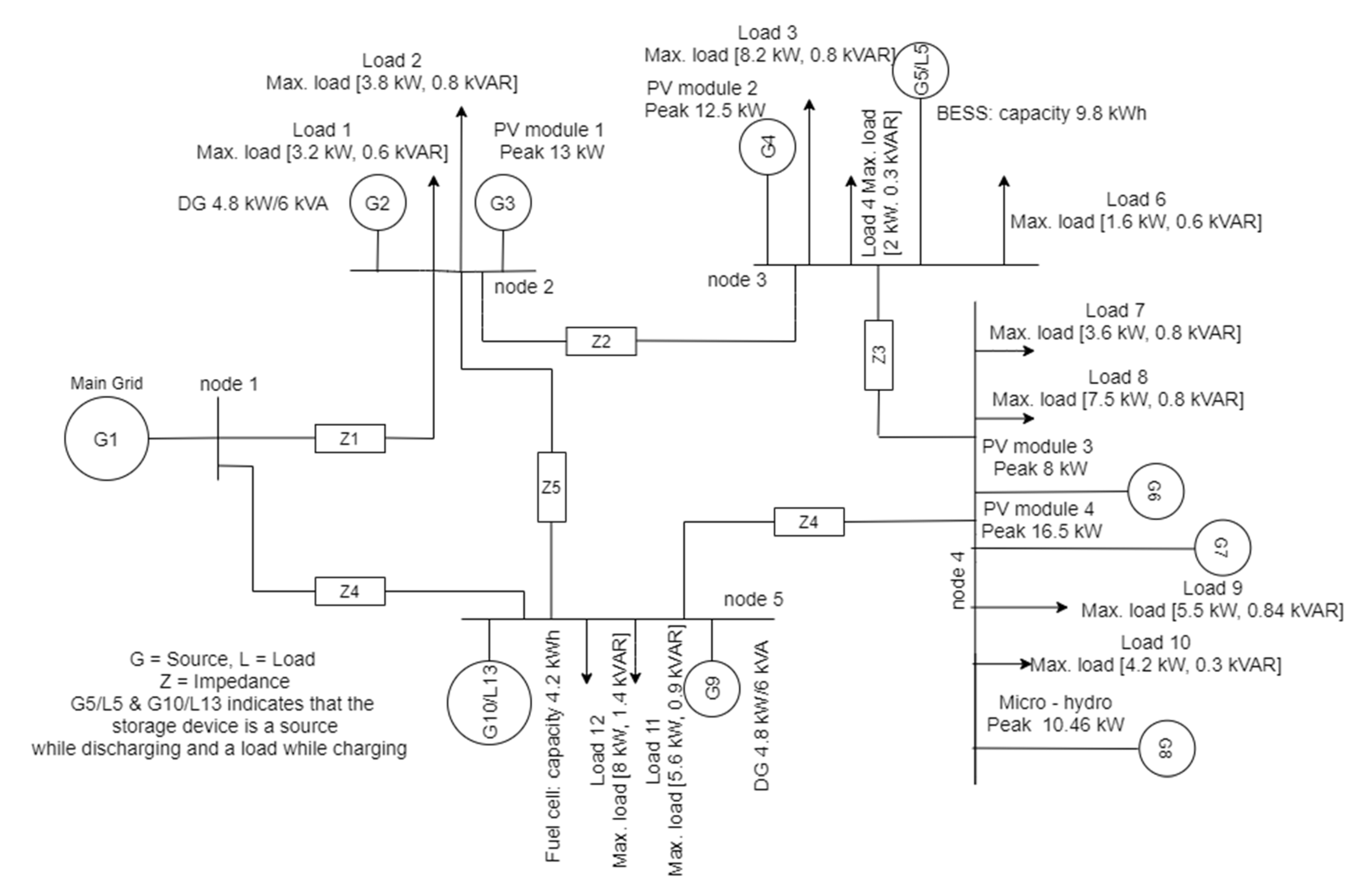
3.1. Microgrid Layout
3.2. Mathematical Model
3.3. LCOE Calculations
- Cc: Initial capital cost (assumed as a single payment in the study)
- Ic: Installation costs
- Fc: Fuel costs
- : Operation and maintenance costs discounted by
4. Generator Models
4.1. Solar PV Panels
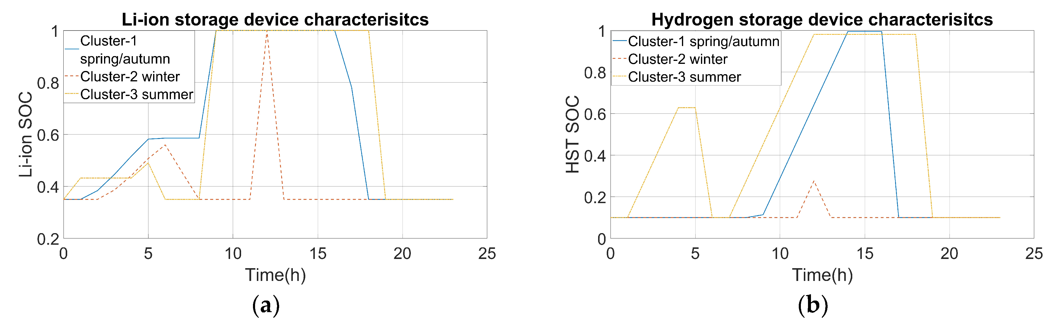
4.2. Li-Ion Storage System (BESS)
4.3. Fuel Cell + Hydrogen Storage Tank
4.4. Diesel Generators (DGs)
4.5. Micro-Hydro Power Plant
5. Results
6. Conclusions
Author Contributions
Funding
Data Availability Statement
Conflicts of Interest
References
- Mosa, M.A.; Ali, A.A. Energy management system of low voltage dc microgrid using mixed-integer nonlinear programing and a global optimization technique. Electr. Power Syst. Res. 2021, 192, 106971. [Google Scholar] [CrossRef]
- Paris Agreement. United Nations Paris Agreement. 2015. Available online: https://unfccc.int/sites/default/files/english_paris_agreement.pdf (accessed on 8 September 2021).
- European Comission. The European Green Deal; European Comission: Brussels, Belgium, 2019. [Google Scholar]
- Ton, D.T.; Smith, M.A. The U.S. Department of Energy’s Microgrid Initiative. Electr. J. 2012, 25, 84–94. [Google Scholar] [CrossRef]
- Marnay, C.; Chatzivasileiadis, S.; Abbey, C.; Iravani, R.; Joos, G.; Lombardi, P.; Mancarella, P.; Von Appen, J. Microgrid evolution roadmap. In Proceedings of the 2015 International Symposium on Smart Electric Distribution Systems and Technologies (EDST), Vienna, Austria, 7–11 September 2015; pp. 139–144. [Google Scholar] [CrossRef]
- Zia, M.F.; Elbouchikhi, E.; Benbouzid, M. Microgrids energy management systems: A critical review on methods, solutions, and prospects. Appl. Energy 2018, 222, 1033–1055. [Google Scholar] [CrossRef]
- Suresh, V.; Janik, P.; Guerrero, J.M.; Leonowicz, Z.; Sikorski, T. Microgrid Energy Management System with Embedded Deep Learning Forecaster and Combined Optimizer. IEEE Access 2020, 8, 202225–202239. [Google Scholar] [CrossRef]
- Vera, Y.E.G.; Dufo-López, R.; Bernal-Agustín, J.L. Energy management in microgrids with renewable energy sources: A literature review. Appl. Sci. 2019, 9, 3854. [Google Scholar] [CrossRef] [Green Version]
- Kaczorowska, D.; Rezmer, J.; Sikorski, T.; Janik, P. Application of PSO algorithms for VPP operation optimization. Renew. Energy Power Qual. J. 2019, 17, 91–96. [Google Scholar] [CrossRef]
- Farinis, G.Κ.; Kanellos, F.D. Integrated energy management system for Microgrids of building prosumers. Electr. Power Syst. Res. 2021, 198, 107357. [Google Scholar] [CrossRef]
- Hou, H.; Xue, M.; Xu, Y.; Xiao, Z.; Deng, X.; Xu, T.; Liu, P.; Cui, R. Multi-objective economic dispatch of a microgrid considering electric vehicle and transferable load. Appl. Energy 2020, 262, 114489. [Google Scholar] [CrossRef]
- Shafik, M.B.; Chen, H.; Rashed, G.I.; El-Sehiemy, R.A. Adaptive multi objective parallel seeker optimization algorithm for incorporating TCSC devices into optimal power flow framework. IEEE Access 2019, 7, 36934–36947. [Google Scholar] [CrossRef]
- Moazeni, F.; Khazaei, J. Dynamic economic dispatch of islanded water-energy microgrids with smart building thermal energy management system. Appl. Energy 2020, 276, 115422. [Google Scholar] [CrossRef]
- Askari, Q.; Younas, I.; Saeed, M. Political Optimizer: A novel socio-inspired meta-heuristic for global. Knowl.-Based Syst. 2020, 195, 105709. [Google Scholar] [CrossRef]
- Niemeyer, L.; Pietronero, L.; Wiesmann, H.J. Fractal Dimension of Dielectric Breakdown. Phys. Rev. Lett. 1984, 52, 1033–1036. [Google Scholar] [CrossRef]
- Witten, T.A.; Sander, L.M. Diffusion-limited aggregation. Phys. Rev. B. 1983, 27, 5686. [Google Scholar] [CrossRef] [Green Version]
- Pereira, J.L.J.; Francisco, M.B.; Diniz, C.A.; Oliver, G.A.; Cunha, S.S.; Gomes, G.F. Lichtenberg Algorithm: A Novel Hybrid PHYSICS-Based Meta-Heuristic for Global Optimization. Expert Syst. Appl. 2020, 170, 114522. [Google Scholar] [CrossRef]
- Gomez-Gonzalez, M.; López, A.; Jurado, F. Optimization of distributed generation systems using a new discrete PSO and OPF. Electr. Power Syst. Res. 2012, 84, 174–180. [Google Scholar] [CrossRef]
- Kim, J.Y.; Mun, K.J.; Kim, H.S.; Park, J.H. Optimal power system operation using parallel processing system and PSO algorithm. Int. J. Electr. Power Energy Syst. 2011, 33, 1457–1461. [Google Scholar] [CrossRef]
- Foltyn, L.; Vysocký, J.; Prettico, G.; Běloch, M.; Praks, P.; Fulli, G. OPF solution for a real Czech urban meshed distribution network using a genetic algorithm. Sustain. Energy, Grids Netw. 2021, 26, 100437. [Google Scholar] [CrossRef]
- García-Muñoz, F.; Díaz-González, F.; Corchero-García, C. A novel algorithm based on the combination of AC-OPF and GA for the optimal sizing and location of DERs into distribution networks. Sustain. Energy Grids Netw. 2021, 27, 100497. [Google Scholar] [CrossRef]
- Branker, K.; Pathak, M.J.M.; Pearce, J.M. A review of solar photovoltaic levelized cost of electricity. Renew. Sustain. Energy Rev. 2011, 15, 4470–4482. [Google Scholar] [CrossRef] [Green Version]
- Jones-albertus, R.; Feldman, D.; Fu, R.; Horowitz, K.; Woodhouse, M. Technology advances needed for photovoltaics to achieve widespread grid price parity. Prog. Photovolt. Res. Appl. 2016, 24, 1272–1283. [Google Scholar] [CrossRef]
- Kumar, P.P.; Saini, R.P. Optimization of an off-grid integrated hybrid renewable energy system with various energy storage technologies using different dispatch strategies. Energy Sources Part A Recover. Util. Environ. Eff. 2020, 32, 1–30. [Google Scholar] [CrossRef]
- Levron, Y.; Guerrero, J.M.; Beck, Y. Optimal Power Flow in Microgrids with Energy Storage. IEEE Trans. Power Syst. 2013, 28, 3226–3234. [Google Scholar] [CrossRef] [Green Version]
- Roque, A.; Sousa, D.M.; Casimiro, C.; Margato, E. Technical and economic analysis of a micro hydro plant—A case study. In Proceedings of the 2010 7th International Conference on the European Energy Market EEM 2010, Madrid, Spain, 23–25 June 2010; pp. 10–15. [Google Scholar] [CrossRef]
- Jasiński, M.; Sikorski, T.; Borkowski, K. Clustering as a tool to support the assessment of power quality in electrical power networks with distributed generation in the mining industry. Electr. Power Syst. Res. 2019, 166, 52–60. [Google Scholar] [CrossRef]
- Jasiński, M.; Sikorski, T.; Kostyła, P.; Leonowicz, Z.; Borkowski, K. Combined Cluster Analysis and Global Power Quality Indices for the Qualitative Assessment of the Time-Varying Condition of Power Quality in an Electrical Power Network with Distributed Generation. Energies 2020, 13, 2050. [Google Scholar] [CrossRef] [Green Version]
- Andrew, N. Machine Learning Yearning, Technical Strategy for AI Engineers in the Era of Deep Learning. 2018. Available online: https://storage.googleapis.com/kaggle-forum-message-attachments/693524/14574/ML_book.pdf (accessed on 8 September 2021).

| Control Variable Values | GA | PSO | PO | LA |
|---|---|---|---|---|
| * PG1 (MW) | 176.45 | 176.76 | 177.39 | 180.45 |
| PG2 (MW) | 48.75 | 49.36 | 48.84 | 47.59 |
| PG5 (MW) | 21.09 | 21.76 | 21.40 | 22.99 |
| PG8 (MW) | 23.20 | 25.73 | 21.69 | 18.30 |
| PG11 (MW) | 12.21 | 11.12 | 12.19 | 12.86 |
| PG13 (MW) | 10.95 | 13.81 | 11.20 | 10.98 |
| V1 (p.u.) | 1.06 | 1.06 | 1.06 | 1.06 |
| V2 (p.u.) | 1.04 | 1.04 | 1.04 | 1.05 |
| V5 (p.u.) | 1.01 | 1.01 | 1.01 | 1.01 |
| V8 (p.u.) | 1.01 | 1.01 | 1.01 | 1.01 |
| V11 (p.u.) | 1.08 | 1.08 | 1.08 | 1.08 |
| V13 (p.u.) | 1.07 | 1.07 | 1.07 | 1.07 |
| T11 | 0.94 | 1.03 | 1.01 | 0.95 |
| T12 | 1.07 | 0.96 | 0.93 | 1.01 |
| T15 | 0.97 | 0.96 | 0.94 | 1.09 |
| T36 | 0.94 | 0.95 | 0.93 | 1.00 |
| Qc10 (MVAr) | 3.26 | 4.77 | 4.61 | 0.23 |
| Qc12 (MVAr) | 4.30 | 4.10 | 5.00 | 3.39 |
| Qc15 (MVAr) | 4.00 | 0.13 | 4.32 | 2.97 |
| Qc17 (MVAr) | 4.85 | 0.04 | 4.92 | 3.55 |
| Qc20 (MVAr) | 4.58 | 3.23 | 4.56 | 4.56 |
| Qc21 (MVAr) | 4.65 | 4.26 | 5.00 | 2.56 |
| Qc23 (MVAr) | 3.27 | 0.28 | 2.71 | 0.81 |
| Qc24 (MVAr) | 1.39 | 4.27 | 3.65 | 3.75 |
| Qc29 (MVAr) | 3.06 | 1.37 | 2.72 | 3.89 |
| Run time (s) | 34.20 | 7.89 | 4.09 | 54.15 |
| Cost ($/h) | 801.6 | 801.7 | 801.6 | 802.8 |
| From | To | Distance (m) | r + jx (Ω) (10−1) |
|---|---|---|---|
| node 1 | node 2 | 180 | 0.455 + 0.147j |
| node 2 | node 3 | 130 | 0.329 + 0.106j |
| node 3 | node 4 | 145 | 0.367 + 0.118j |
| node 4 | node 5 | 195 | 0.493 + 0.159j |
| node 5 | node 1 | 140 | 0.354 + 0.114j |
| node 2 | node 5 | 190 | 0.481 + 0.155j |
| Parameters | Value | Parameters | Value |
|---|---|---|---|
| Capital cost of PV panels | 0.6 $/kW | Annual O&M for entire installation | 141 $ |
| Annual O&M costs of PV | 6.5 $/module | Erection cost of FC + HST + electrolyzer | 5% of capital cost of entire FC installation |
| Total installed capacity | 48.9 kW | Fuel cost of FC + HST | 1 0.033 times the energy consumed |
| Erection cost PV system | 20% of capital cost of PV system | Electrolyzer replacement cost | Cost of replacement at capital cost at discounted rate |
| Capital cost of BSS | 1500 $ | Capital cost of DG | 2099 $/unit |
| Erection cost of BSS | 5% of capital cost of BSS | Total number of units | 2 |
| Fuel cost of BSS | 1 0.033 time the energy consumed | Replacement cost | Cost of replacement at capital cost at discounted rate |
| O&M costs of BSS | Cost of replacement at capital cost at discounted rate | O&M cost for DGs | 1020 $ |
| Capacity of BSS | 9.8 kWh | Fuel Cost of DG | Calculated based on yearly fuel consumption |
| Capital cost of FC | 2400 $/kW | Capital cost of Francis turbine | 15,200 $ |
| Installed capacity of FC | 3 kW | Total installed capacity | 11.6 kW |
| Capital cost of electrolyzer | 800 $/kW | Erection cost for Francis turbine | 20% of capital cost of turbine |
| Installed rating of electrolyzer | 3 kW | Annual O&M costs | 1216 $ |
| Capital cost of HST | 600 $ | Replacement cost | No replacement, life > 25 years |
Publisher’s Note: MDPI stays neutral with regard to jurisdictional claims in published maps and institutional affiliations. |
© 2021 by the authors. Licensee MDPI, Basel, Switzerland. This article is an open access article distributed under the terms and conditions of the Creative Commons Attribution (CC BY) license (https://creativecommons.org/licenses/by/4.0/).
Share and Cite
Suresh, V.; Jasinski, M.; Leonowicz, Z.; Kaczorowska, D.; J., J.; Reddy K., H. Political-Optimizer-Based Energy-Management System for Microgrids. Electronics 2021, 10, 3119. https://doi.org/10.3390/electronics10243119
Suresh V, Jasinski M, Leonowicz Z, Kaczorowska D, J. J, Reddy K. H. Political-Optimizer-Based Energy-Management System for Microgrids. Electronics. 2021; 10(24):3119. https://doi.org/10.3390/electronics10243119
Chicago/Turabian StyleSuresh, Vishnu, Michal Jasinski, Zbigniew Leonowicz, Dominika Kaczorowska, Jithendranath J., and Hemachandra Reddy K. 2021. "Political-Optimizer-Based Energy-Management System for Microgrids" Electronics 10, no. 24: 3119. https://doi.org/10.3390/electronics10243119
APA StyleSuresh, V., Jasinski, M., Leonowicz, Z., Kaczorowska, D., J., J., & Reddy K., H. (2021). Political-Optimizer-Based Energy-Management System for Microgrids. Electronics, 10(24), 3119. https://doi.org/10.3390/electronics10243119