Resource Allocation in NOMA-Assisted Ambient Backscatter Communication System

Abstract

This paper considers a non-orthogonal multiple access (NOMA)-assisted ambient backscatter communication (AmBC) system. To maximize the achievable sum rate (ASR) of the AmBC system, a joint optimization problem over a backscatter device (BD) grouping strategy, reflection coefficients, and decoding order is formulated, where the BD grouping strategy contains the number of BD groups and the BD allocation strategy. The BD grouping strategy, the reflection coefficients, and the decoding order are all intertwined, and the global search is extremely complex. As a result, we propose a four-step optimization algorithm. First, we give the closed-form optimal solution of the BD decoding order and reflection coefficient for a given grouping strategy. Then, for a given number of BD groups, we propose a low-complexity BD allocation strategy based on the complexity–performance trade-off. Finally, the number of BD groups with the largest ASR is selected as the global optimal number of BD groups. The simulation results show that the proposed four-step optimization algorithm is better than the benchmark solution.

1. Introduction

As a low-complexity, low-power Internet of Things (IoT) communication technology, ambient backscatter communication (AmBC) [1] has attracted widespread interest. The basic concept of AmBC is to modulate its information to the ambient radio frequency (RF) source signal by changing the load impedance of the backscattering device (BD) to enable information transmission [2]. AmBC is a potential technology for the green IoT [3], which can improve spectrum efficiency and energy efficiency at the same time. The development of AmBC will greatly promote the widespread popularity of the IoT.

In the AmBC system, BR will receive two types of signals: the backscatter signal from BD and the broadcast signal from RF. There are mainly two ways to demodulate BD signals, namely, energy detector [4] and cooperative receiver [5]. Typically, energy detectors are employed to acquire BD information by considering RF signals as interference. Therefore, traditional AmBC systems with energy detectors have extremely low transmission rates [4]. The cooperative receiver recovers the RF and BD signals [6] by using successive interference cancellation (SIC) [5], which can effectively improve the throughput of the AmBC system. Although the cooperative receiver is more complicated than the energy detector, its transmission rate has been greatly improved. Therefore, we will focus on the AmBC system with cooperative receivers.

In response to the growing demand for IoT, 5 G/6 G wireless communications should meet increasingly demanding requirements, such as massive connectivity and high spectral efficiency and high throughput [7,8]. Similarly, the AmBC system as one of the solutions for the IoT also faces the same problems mentioned above. Consequently, non-orthogonal multiple access (NOMA) should be introduced into AmBC systems to increase the number of IoT device accesses while also improving spectrum efficiency [9]. Unlike orthogonal multiple access (OMA), which enables each RB to serve just one user, power-domain NOMA (PD-NOMA) allows each RB to serve multiple users at various power levels simultaneously [10]. Therefore, we focus on the PD-NOMA-assisted AmBC system in this paper. Unless otherwise stated, all references to NOMA in this paper refer to PD-NOMA. Since both NOMA and AmBC systems with cooperative receivers use SIC for signal decoding, using NOMA to assist AmBC systems can further improve spectral efficiency without increasing the complexity of BD. Unlike traditional NOMA systems, BDs in NOMA-assisted AmBC systems transmit data by reflecting RF signals and adjusting the reflection coefficient for power control [11]. The signal strength of the BD received by the BR is not only related to the path loss of the BD–BR link but also related to the path loss of the BD–RF link [12]. Therefore, the decoding order should consider the above two path losses and the reflection coefficient. Finally, as the number of BDs increases, it is undoubtedly unrealistic to simultaneously transmit data in the same resource block, so it is necessary to use a solution combining NOMA and OMA for data transmission as in [13]. Therefore, BDs need to be grouped. BDs in the same group use the NOMA scheme for transmission, and BDs in different groups use the OMA scheme for data transmission. In this paper, we propose a novel NOMA-assisted AmBC system to maximize the achievable sum rate (ASR). The main contributions of this paper are as follows.

(1)

We innovatively proposed the NOMA-assisted AmBC system. As far as we know, no research has been conducted to apply NOMA to the AmBC system to increase its ASR. Compared with the traditional AmBC system, the proposed system can significantly improve the ASR of the AmBC system.

(2)

To maximize the ASR of the AmBC system, we formed a joint optimization problem on the BD grouping strategy, reflection coefficient, and decoding order. The BD grouping strategy contains the number of BD groups and the BD allocation strategy. To simplify this problem, we converted the above problem into a four-step optimization problem. The computational complexity can be significantly reduced by solving the described four-step optimization problem.

(3)

Under the static grouping strategy, i.e., when the number of BD groups and the BD allocation strategy are known, we give the closed-form solutions for the optimal decoding order and reflection coefficients of BDs.

(4)

Under the dynamic grouping strategy, the BD grouping strategy is divided into two steps: the number of BD groups strategy and the BD allocation strategy. Therefore, for a given number of BD groups, we propose a low-complexity BD allocation strategy based on the complexity–performance trade-off. Once the BD allocation strategy is determined, we can solve for the optimal ASR based on the static grouping strategy. Then, the number of BD groups with the maximum ASR is selected as the global optimal number of BD groups.

The rest of this paper is organized as follows. Related work is introduced in Section 2. Section 3 introduces the system model and problem formulation. Section 4 presents the static BD grouping solution, while Section 5 presents the dynamic BD grouping solution. Section 6 presents the numerical results. Finally, Section 7 concludes the paper.

2. Related Work

Monostatic backscatter communications (MBC), bistatic backscatter communications (BBC), and AmBC are the three major types of backscatter communications [1]. In MBC, the cost of the reader is high, because both the RF source and the BD are on the reader (BR), and the modulated signal may be affected by round-trip route loss, so it is only suitable for short-range communication [14]. In contrast to MBC, the BBC’s carrier transmitter and BR are separate, and the BBC’s performance can be greatly improved by adjusting the position of the carrier transmitter. Although the carrier transmitter is big and expensive to deploy, the BBC carrier transmitter and backscatter receiver have a lower manufacture cost than the MBC [15]. The carrier transmitter is not needed in AmBC [16], as opposed to BBC, since data transmission is accomplished via the use of ambient RF sources, such as Wi-Fi access points (APs), cellular base stations (BSs), and TV towers. As a result, the AmBC has some benefits over the BBC. First, AmBC utilizes existing RF sources and does not require the deployment of dedicated RF sources, which reduces the deployment and maintenance costs of AmBC. Second, AmBC uses existing RF sources for transmission and does not require separate spectrum for AmBC, which may result in increased spectrum utilization.

The application of NOMA to backscatter communication can further advance the development of large-scale, low-power IoT [16]. Ref. [17] discuss the benefits and drawbacks of using NOMA with backscatter communication systems. Meanwhile, [18] consider the resource allocation problem in the NOMA-assisted backscatter communication network based on quality of service (QoS). Building on these findings, [19] propose a novel approach for estimating the capacity of NOMA-assisted backscatter communication systems. In addition, [20] optimize the reflection coefficient of the backscatter tag to increase the security of NOMA-assisted backscatter transmission. Using another approach, [21] consider various QoS requirements for bistatic backscatter communication of roadside sensors and propose an alternate optimization framework for maximizing the energy efficiency of the network. Based on the downlink of NOMA-assisted backscatter communication systems, [16] generated a closed-form formula for the system capacity and outage probability for the single base station antenna situation. Then, [22] extended [16] to multiple base station antennas and found that increasing the number of base station antennas improves the performance of the backscattered communication systems. Meanwhile, [23] examine the resource allocation issue in a NOMA-assisted backscatter communication system and optimize the network’s performance by adjusting various network parameters. NOMA is used in [24] to assist the BD in communication, where the BD uses the signal from one cellular user as an RF source for data transmission, and the base station sends data to multiple other cellular users based on NOMA. [25] consider a backscattered communication system with NOMA-enhanced BDs transmitting to a BR using a protocol that combines NOMA and dynamic time division multiple access. However, the NOMA-assisted backscatter communication discussed in [17,18,19,20,21,22,23,24,25] is based on the BBC system, not the AmBC system. The optimization method of the NOMA-assisted AmBC system is different from that of the NOMA-assisted BBC system. [26] study the NOMA-assisted AmBC with imperfect continuous interference cancellation (SIC) decoding and proposed a method to maximize the sum rate of the system. Meanwhile, [27] study the trade-off between safety and reliability in the presence of in-phase and quadrature phase imbalance in the NOMA-assisted AmBC network. In addition, [28] introduce backscatter communication in the multi-unit IoT assisted by NOMA, which maximizes the total energy efficiency of the IoT network under the premise of ensuring QoS. Building on this concept, [29,30] provide green solutions for AmBC-enabled NOMA networks under imperfect SIC decoding by jointly optimizing the transmission power of the base station and the reflection coefficient of the BD to maximize the system performance. [31] explore RF-powered cognitive radio networks (CRNs) with NOMA to achieve optimum throughput by determining the best allocation of time resources between harvest-then-transmit (HTT) and AmBC modes within the strict transmit power restriction of BDs. Overall, [16,17,18,19,20,21,22,23,24,25,26,27,28,29,30,31] greatly promote the combination of NOMA and backscatter communication and promote the further development of IoT. However, to the best of our knowledge, no study has been conducted to improve the performance of NOMA-assisted AmBC, which decodes multiple BDs and an RF signal in BR with NOMA.

3. System Model and Problem Formulation

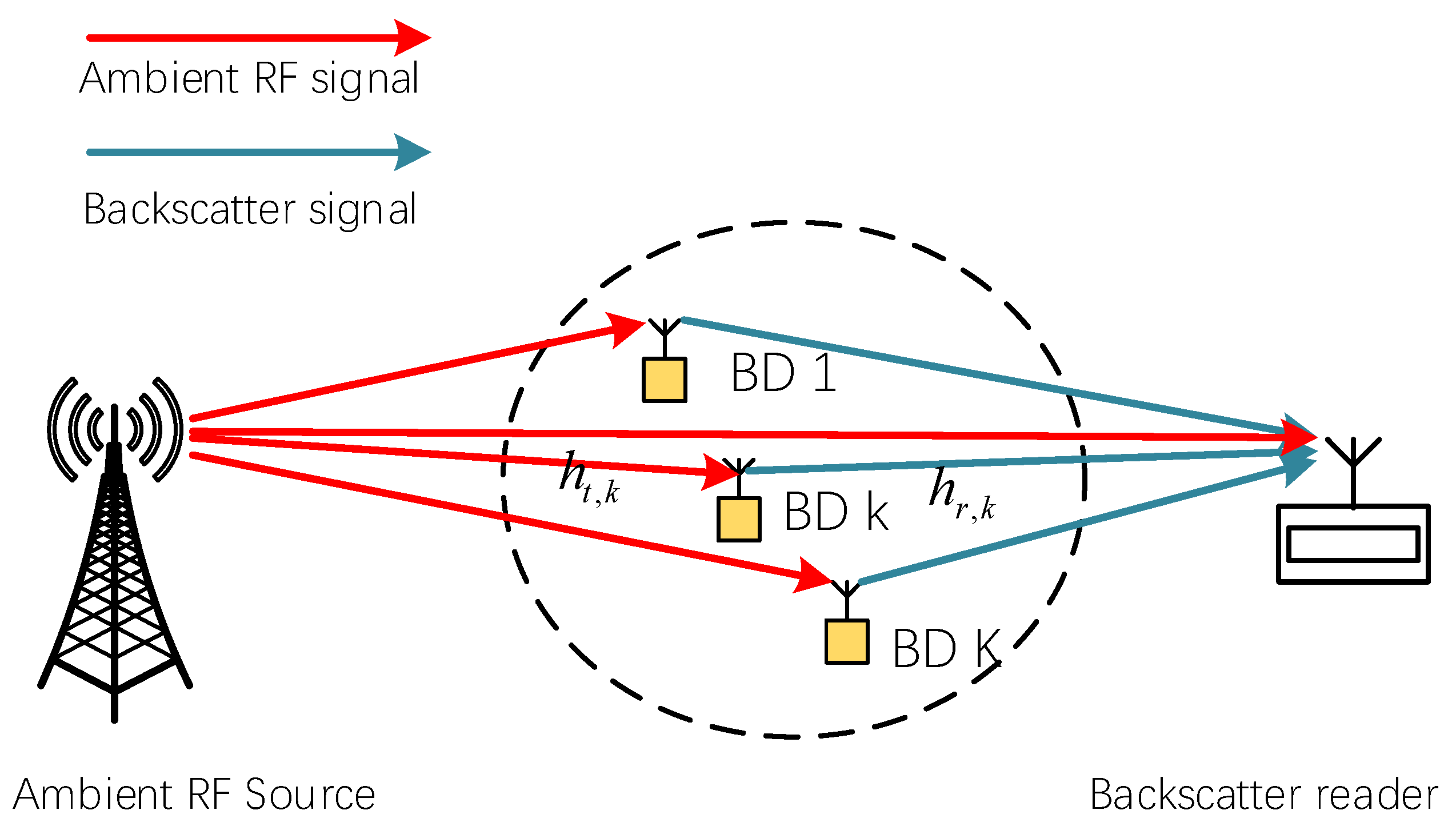
3.1. System Model

As shown in Figure 1, we consider a NOMA-assisted AmBC system, which consists of an ambient RF source, a BR, and $K$ BDs. The RF source transmits broadcast signals, while BDs modulate information on the incident single by intelligently changing its load impedance. In the proposed NOMA-assisted AmBC system, multiple BDs transmit data to the BD based on a protocol that integrates NOMA and dynamic time division multiple access (TDMA). Each of the ambient RF source’s BDs and BR are equipped with only one antenna. We assume that the dynamic TDMA can be equally divided into $M$ RBs, where $M\le K$ can change dynamically with the demand of the BD group. The BDs may be dynamically split into $M$ groups based on the number of RBs, with one group allocated one RB. BDs in the same group perform NOMA transmission, and BDs in different groups perform OMA transmission.

Let $s_0$ be the symbol transmitted by the ambient RF resource. We assume that the effect of signal reflection between BDs can be ignored. Then, the received signal of the $k$th BD is expressed as

$$x_{t,k}=h_{t,k}\sqrt{P_t}{s}_0,$$

(1)

where $P_t$ is the transmit power of the RF source. Given that BD is passive, a part of the energy from the incident signal should be harvested by BD in order to maintain proper operation of backscatter communication. We denote $E_k$ as the minimal power needed to keep the BD circuit running. To make the BD circuit operate normally, the following conditions should be met:

$$\eta \left(1-a_k\right)P_t{\left|h_{t,k}\right|}^2\ge E_k,$$

(2)

where $\eta \in \left[0,1\right]$ is the energy-harvesting efficiency, $a_k\in \left(0,1\right)$ is the reflection coefficient, and $h_{t,k}\in {ℂ}^{1\times 1}$ is the channel gain between the ambient RF source and the $k$th BD. Assuming that the BD transmission has the same symbol rate as the RF source, the backscatter signal of the $k$th BD can be expressed as

$$x_{r,k}=\sqrt{a_k}{x}_{t,k}{s}_k,$$

(3)

where $s_k$ is the information symbol transmitted by the $k$th BD. Then, the signal received by BR in the $m$th RB can be given by

$$y_m={\displaystyle \sum }_{k=1}^K{u}_{m,k}{h}_{r,k}{x}_{r,k}+h_t\sqrt{P_t}{s}_0+z_m,$$

(4)

where $h_0\in {ℂ}^{1\times 1}$and $h_{r,k}\in {ℂ}^{1\times 1}$ are the channel gains from the RF to BR and the $k\mathrm{th}$ BD to BR, respectively,$u_{m,k}\in \left\{0,1\right\}$ is the indicator representing that BD $k$ is assigned to the$m$th group, $z_m$ is white Gaussian noise with zero mean and variance ${\sigma }^2$.

The RB employs the SIC to decode the signals of all BDs in the same RB. Obviously, before decoding the BD signal, the ambient RF signal needs to be decoded. We denote the signal-to-interference-plus-noise ratio (SINR) received by the BR about the ambient RF source signal in the $m$th RB as $SIN{R}_{m,t}$; then, we can get

$$SIN{R}_{m,t}=\frac{{\left|h_0\right|}^2{P}_t}{{{\displaystyle \sum }}_{k=1}^K{u}_{m,k}{\left|h_{t,k}{h}_{r,k}\right|}^2{a}_k{P}_t+{\sigma }^2},$$

(5)

where $h_0$ is the channel gain between the ambient RF source and the BR. Denote the minimum SINR requirement to decode the signal of the ambient RF source in the $m$th RB as ${\gamma }_t$. Then, to decode the signal $s_0$, the following restrictions should be satisfied., i.e.,

$$SIN{R}_{m,t}\ge {\gamma }_t, \forall m.$$

(6)

Let ${\pi }_{m,k}$ denote the decoding order for the BD $k$ in $m$th RB, where ${\pi }_{m,k}=n$ indicates that the signal of BD $k$ is the $n$th signal to be decoded in the $m$th RB. Then, the received SINR to decode the signal of BD $k$ can be written as

$$SIN{R}_{m,k}=\frac{a_k{\left|h_{t,k}{h}_{r,k}\right|}^2{P}_t}{{{\displaystyle \sum }}_{{\pi }_{m,j}>{\pi }_{m,k}>0}{\left|h_{t,j}{h}_{r,j}\right|}^2{a}_j{P}_t+{\sigma }^2}.$$

(7)

Denote the minimum SINR requirement to decode the signal of the BD $k$ as ${\gamma }_k$; then, the $SIN{R}_{m,k}$ needs to satisfy the following conditions:

$$SIN{R}_{m,k}\ge {\gamma }_k,\forall k.$$

(8)

Then, the ASR of BD $k$, based on dynamic TDMA and NOMA protocols, can be represented as

$$R_{m,k}=\frac{1}{M}lo{g}_2\left(1+\frac{a_k{\left|h_{t,k}{h}_{r,k}\right|}^2{P}_t}{{{\displaystyle \sum }}_{{\pi }_{m,j}>{\pi }_{m,k}>0}{\left|h_{t,j}{h}_{r,j}\right|}^2{a}_j{P}_t+{\sigma }^2}\right).$$

(9)

It is assumed that the system can obtain all CSI and SIC can completely eliminate interference. Then, the ASR of the AmBC system in the $mth$ RB can be given by:

$$R_m={\displaystyle \sum }_{u_{m,k}=1}{R}_{m,k} =\frac{1}{M}lo{g}_2\left(1+{\displaystyle \sum }_{u_{m,k}=1}\frac{a_k{\left|h_{t,k}{h}_{r,k}\right|}^2{P}_t}{{\sigma }^2}\right).$$

(10)

3.2. Problem Formulation

The objective of this paper is to optimize the ASR of the AmBC system by adjusting the number of BD groups $M$, the BD grouping variables $\left\{u_{m,k}\right\}$, the reflection coefficients $\left\{a_k\right\}$, and the decoding order $\left\{{\pi }_{m,k}\right\}$. Then, the optimization problem can be stated as follows.

$$P1: \underset{\left\{u_{m,k}\right\}, \left\{{\pi }_{m,k}\right\},\left\{a_k\right\},M}{\mathrm{Maximize}} R_{sum}={\displaystyle \sum }_{m=1}^M{R}_m$$

(11a)

$$s.t. \left(1-a_k\right){\left|h_{t,k}\right|}^2{P}_t\ge E_k, u_{m,k}=1$$

(11b)

$$SIN{R}_{m,k}\ge {\gamma }_k,\forall k,$$

(11c)

$$SIN{R}_t\ge {\gamma }_t,$$

(11d)

$$1\ge a_k\ge 0,\forall k,$$

(11e)

$$u_{m,k}\in \left\{0,1\right\},$$

(11f)

$${\displaystyle \sum }_{m=1}^M{u}_{m,k}=1,\forall k,$$

(11g)

$$M\in \left\{1,\dots ,K\right\}.$$

(11h)

Obviously in problem P1, the optimization variables, i.e., the number of BD groups $M$, BD grouping variables $\left\{u_{m,k}\right\}$, the reflection coefficients $\left\{a_k\right\}$, and the decoding order $\left\{{\pi }_{m,k}\right\}$, are intertwined, which makes the problem tricky. The optimal solution of problem P1 may be solved by the exhaustive method. However, the difficulty of doing so is definitely great. Therefore, a low-complexity solution needs to be found.

4. Static BD Grouping Solutions

However, when number of BD groups $M$ and BD grouping variables $\left\{u_{m,k}\right\}$ are determined, we can see that the reflection coefficients $\left\{a_k\right\}$ and the decoding order $\left\{{\pi }_{m,k}\right\}$ among different groups are independent of each other. It is worth noting that we can find the best strategies for the reflection coefficients $\left\{a_k\right\}$ and the decoding order $\left\{{\pi }_{m,k}\right\}$ for any given numbers of BD groups $M$ and given BD grouping variables $\left\{u_{m,k}\right\}$. When the grouping policy of BD is static, we can give the optimal reflection coefficients $\left\{a_k\right\}$ and decoding order $\left\{{\pi }_{m,k}\right\}$.

When the number of BD groups $M$ and the BD grouping variables $\left\{u_{m,k}\right\}$ are given, maximizing $R_m$ is equivalent to maximizing ${\displaystyle \sum }_{u_{m,k}=1}{a}_k{\left|h_{t,k}{h}_{r,k}\right|}^2{P}_t$. Then, for the $mth$ RB, the optimization problem can be expressed as follows.

$$P2: \underset{ \left\{{\pi }_{m,k}\right\},\left\{a_k\right\}}{\mathrm{Maximize}} {\displaystyle \sum }_{u_{m,k}=1}{a}_k{\left|h_{t,k}{h}_{r,k}\right|}^2{P}_t$$

(12a)

$$s.t. \left(1-a_k\right){\left|h_{t,k}\right|}^2{P}_t\ge E_k, k\in G_m,$$

(12b)

$$SIN{R}_{m,k}\ge {\gamma }_k, k\in G_m,$$

(12c)

$$SIN{R}_t\ge {\gamma }_t, k\in G_m,$$

(12d)

$$1\ge a_k\ge 0,k\in G_m,$$

(12e)

where $G_m$ denotes the set of the BD in the $mth$ group.

4.1. Decoding Order

Given that different BD decoding orders affect the received power of BR, we should first determine the optimal decoding order. The following theorem is provided to find the best decoding order.

Theorem 1.

The decreasing order of $\left({\left|h_{t,k}\right|}^2{P}_t-E_k\right){\left|h_{r,k}\right|}^2\left(1+\frac{1}{{\gamma }_k}\right)$is an optimal decoding order for Problem P2.

Proof. 

The proof process is similar to [12]. Assume that BD $i$ and BD $j$ are two BDs in group $m$ with adjacent decoding order. Then, there may be two cases in the decoding order. In Case 1, BD $i$ is decoded first, and in Case 2, BD $j$ is decoded first. Let $P_s$ be the sum of the power received by BR from BD $i$ and BD $j$, we can get

$$P_s=a_i{\left|h_{t,i}{h}_{r,i}\right|}^2{P}_t+a_j{\left|h_{t,j}{h}_{r,j}\right|}^2{P}_t.$$

(13)

When the effect of the decoding order of BD $i$ and BD $j$ on P3 is considered, the optimization problem can be reformulated as

$$P3:\underset{ \left\{{\pi }_{m,k}\right\},\left\{a_k\right\}}{\mathrm{Maximize}} P_s$$

(14a)

$$s.t. \left(1-a_k\right){\left|h_{t,k}\right|}^2{P}_t\ge E_k, k=\left\{i, j\right\}$$

(14b)

$$SIN{R}_{m,k}\ge {\gamma }_k, k=\left\{i, j\right\}$$

(14c)

$$P_s+I+{\sigma }^2\ll w, k=\left\{i, j\right\}$$

(14d)

$$1\ge a_k\ge 0, k=\left\{i, j\right\}$$

(14e)

where $I$ is the interference from BDs with a higher decoding order than BD $i$ and BD $j$, $w$ is the upper bound of the SINR constraint for BD with a decoding order less than BD $i$ and BD $j$, and ${\gamma }_i$ and ${\gamma }_j$ are the minimum SINR requirements for BD $i$ and BD $j$. □

Case 1: Assume that the signal of BD $i$ is decoded first. Based on the constraints in problem P3, the feasible domain of the reflection coefficients is as follows.

$$\mathit{C}\mathbf{1}:\{\begin{array}{}\mathrm{(15a)}& \frac{a_i{\left|h_{t,i}{h}_{r,i}\right|}^2{P}_t}{a_j{\left|h_{t,j}{h}_{r,j}\right|}^2{P}_t+{\sigma }^2+I}\ge {\gamma }_i,\hfill \mathrm{(15b)}& \frac{a_j{\left|h_{t,j}{h}_{r,j}\right|}^2{P}_t}{{\sigma }^2+I}\ge {\gamma }_j,\hfill \mathrm{(15c)}& \left(1-a_i\right){\left|h_{t,i}\right|}^2{P}_t\ge E_i,\hfill \mathrm{(15d)}& \left(1-a_j\right){\left|h_{t,j}\right|}^2{P}_t\ge E_j,\hfill \mathrm{(15e)}& a_i{\left|h_{t,i}{h}_{r,i}\right|}^2{P}_t+a_j{\left|h_{t,j}{h}_{r,j}\right|}^2{P}_t+I+{\sigma }^2\ll w\hfill \end{array}$$

According to Equations (15a) and (15b), the lower bounds for $a_i$ and $a_j$ are

$$a_i^l=\frac{{\gamma }_i({\gamma }_j+1)\left({\sigma }^2+I\right)}{{\left|h_{t,i}{h}_{r,i}\right|}^2{P}_t},$$

(16)

$$a_j^l=\frac{{\gamma }_j\left({\sigma }^2+I\right)}{{\left|h_{t,j}{h}_{r,j}\right|}^2{P}_t}.$$

(17)

According to Equation (15c), the upper bound of $a_i$ is given by

$$a_i^u=1-\frac{E_i}{{\left|h_{t,i}\right|}^2{P}_t}.$$

(18)

Then, the upper bound of $a_j$ based on Equations (15a), (15d), and (18) is given by

$$a_j^u=\min \left\{1-\frac{E_j}{{\left|h_{t,j}\right|}^2{P}_t},\frac{a_i^u{\left|h_{t,i}{h}_{r,i}\right|}^2{P}_t-{\sigma }^2-I}{{\gamma }_i{\left|h_{t,j}{h}_{r,j}\right|}^2{P}_t}\right\}.$$

(19)

Note that if the problem P2 has a feasible region, the lower bounds and upper bounds of $a_i$ and $a_j$ need to meet $0\ll a_i^l\ll a_i^u\ll 1$ and $0\ll a_j^l\ll a_i^u\ll 1$. Next, we need to consider the case where Case 1 has a feasible region. Obviously, $P_s$ increases with the increase in $a_i$ and $a_j$. When $a_i$ and $a_j$ obtain the upper bound, $P_s$ subsequently obtains the upper bound. Substituting $a_i^u$ and $a_j^u$ into $P_s$, we can obtain the maximum $P_s$for Case 1. Denote the maximum $P_s$ in Case 1 as $mr{p}_1$; then, we can get

$$P_s^1=\min \left\{c_0,c_1,w-I-{\sigma }^2\right\},$$

(20)

where $c_0$ and $c_1$ are given by

$$c_0=\left({\left|h_{t,i}\right|}^2{P}_t-E_i\right){\left|h_{r,i}\right|}^2+\left({\left|h_{t,j}\right|}^2{P}_t-E_j\right){\left|h_{r,j}\right|}^2,$$

(21)

$$c_1=\left({\left|h_{t,i}\right|}^2{P}_t-E_i\right){\left|h_{r,i}\right|}^2\left(1+\frac{1}{{\gamma }_i}\right)-I-{\sigma }^2.$$

(22)

Case 2: Assume that the signal of BD $j$ is decoded first. Based on the constraints in problem P3, the feasible domain of the reflection coefficients is as follows.

$$\mathit{C}\mathbf{2}:\{\begin{array}{}\mathrm{(23a)}& \frac{a_j{\left|h_{t,j}{h}_{r,j}\right|}^2{P}_t}{a_i{\left|h_{t,i}{h}_{r,i}\right|}^2{P}_t+{\sigma }^2+I}\ge {\gamma }_j,\hfill \mathrm{(23b)}& \frac{a_i{\left|h_{t,i}{h}_{r,i}\right|}^2{P}_t}{{\sigma }^2+I}\ge {\gamma }_i,\hfill \mathrm{(23c)}& \left(1-a_i\right){\left|h_{t,i}\right|}^2{P}_t\ge E_i,\hfill \mathrm{(23d)}& \left(1-a_j\right){\left|h_{t,j}\right|}^2{P}_t\ge E_j,\hfill \mathrm{(23e)}& a_i{\left|h_{t,i}{h}_{r,i}\right|}^2{P}_t+a_j{\left|h_{t,j}{h}_{r,j}\right|}^2{P}_t+I+{\sigma }^2\ll w.\hfill \end{array}$$

The maximum $P_s$ for Case 2 can be obtained using the same method as in Case 1. Denote the maximum $P_s$ in Case 1 as $P_s^2$; then, we can get

$$P_s^2=\min \left\{c_0,c_2,w-I-{\sigma }^2\right\},$$

(24)

where $c_2$ can be obtained by

$$c_2=\left({\left|h_{t,j}\right|}^2{P}_t-E_j\right){\left|h_{t,j}\right|}^2\left(1+\frac{1}{{\gamma }_j}\right)-I-{\sigma }^2.$$

(25)

Comparing Equation (20) with Equation (24), we can find that when $c_1\ge c_2$ $ms{p}_1\ge ms{p}_2$. Denote $P_s^m$ as the maximum $P_s$ in the two cases, then, we can get

$$P_s^m=\{\begin{array}{c}{P}_s^1, c_1 \ge c_2\\ P_s^2, c_1<c_2\end{array}.$$

(26)

Based on the above analysis, P3 has more gain when the BD with larger $\left({\left|h_{t,k}\right|}^2{P}_t-E_k\right){\left|h_{r,k}\right|}^2\left(1+\frac{1}{{\gamma }_k}\right)$ is decoded. Let

$${\varrho }_k=\left({\left|h_{t,k}\right|}^2{P}_t-E_k\right){\left|h_{r,k}\right|}^2\left(1+\frac{1}{{\gamma }_k}\right).$$

(27)

We can conclude that the decreasing order of ${\varrho }_k$ is the optimal decoding order of BD. Arrange ${\varrho }_k$ in descending order and denote the position of ${\varrho }_k$ in the order as $l\left({\varrho }_k\right)$. Then, the optimal decoding order of BD $k$ in group $m$ is given by

$${\pi }_{m,k}=l\left({\varrho }_k\right).$$

(28)

Without sacrificing generality, we suppose that group $m$ contains $N$ BDs. Then, the suggested decoding order approach is described in Algorithm 1.

Algorithm 1. Proposed decoding order algorithm

Input: $N$, $P_t$,$E_k$,$\{h_{t,k}$}, {$h_{r,k}$}, {${\gamma }_k$}

1: For$k=1: N$ do

2:  Calculate ${\varrho }_k$ according to Equation (27);

3: End for

4: Arrange ${\varrho }_k$ in descending order and get $l\left({\varrho }_k\right)$;

5: ${\pi }_{m,k}=l\left({\varrho }_k\right)$;

Output:$\left\{{\pi }_{m,k}\right\}$

4.2. Reflection Coefficient

The optimal decoding order was determined in the previous section, and the optimal reflection coefficient setting will be studied in this section. Assume that there are $N$ BDs in the mth RB without compromising generality. Following the determination of the decoding order of BDs by Algorithm 1, the BD is labeled as its decoding order. Thus, for BDs in the $mth$ RB, the P2 can be converted into the following problem.

$$P4:\underset{ \left\{a_n\right\}}{\mathrm{Maximize}} {\displaystyle \sum }_{n=1}^N{a}_n{\left|h_{t,n}{h}_{r,n}\right|}^2{P}_t$$

(29a)

$$s.t. \left(1-a_n\right){\left|h_{t,n}\right|}^2{P}_t\ge E_n,\forall n,$$

(29b)

$$SIN{R}_{m,n}\ge {\gamma }_n,\forall n,$$

(29c)

$$SIN{R}_t\ge {\gamma }_t,$$

(29d)

$$1\ge a_n\ge 0,\forall n,$$

(29e)

$$n=1,2,\dots ,N.$$

(29f)

To ensure that all BDs can be decoded, then $SIN{R}_{m,n}$ and $SIN{R}_t$ should satisfy constraint Equations (29c) and (29d). To facilitate the analysis, we combine the constraints Equations (29c) and (29d) into the following form.

$$SIN{R}_{m,n}\ge {\gamma }_n,\forall n=\left\{0,1,2,..,N\right\},$$

(30)

where $SIN{R}_{m,0}=SIN{R}_t$ and $r_0={\gamma }_t$. For ease of analysis, $R_{m,n}$ can be re-expressed as

$$SIN{R}_{m,n}=\frac{a_n{\left|h_n\right|}^2{P}_t}{{{\displaystyle \sum }}_{i=n+1}^{i=N}{\left|h_i\right|}^2{a}_i{P}_t+{\sigma }^2},\forall n=\left\{0,1,2,\dots ,N\right\},$$

(31)

where$a_0=1$,$h_i=h_{t,i}{h}_{r,i}$. Then, problem P3 can be rewritten as

$$P5: \underset{ \left\{a_n\right\}}{\mathrm{Maximize}} {\displaystyle \sum }_{n=1}^N{a}_n{\left|h_n\right|}^2$$

(32a)

$$s.t. \left(1-a_n\right){\left|h_{t, n}\right|}^2{P}_t\ge E_n,\forall n,$$

(32b)

$$SIN{R}_{m,n}\ge {\gamma }_n,\forall n,$$

(32c)

$$1\ge a_n\ge 0,\forall n,$$

(32d)

$$n=0,1,2,\dots ,N,$$

(32e)

where $E_0=0$. To find the solutions to problem P5, we should first determine the boundary conditions of $a_n,n\in \left\{1,\dots ,N\right\}$. The upper bound of problem P5 can be obtained by (32b). Then, the upper bound of $a_n$ may be written as

$$a_n^u=1-\frac{E_n}{{\left|h_{t, n}\right|}^2{P}_t}.$$

(33)

Similarly, we also need to get the lower bound of $a_n$. BD signals are decoded in descending order from smallest to biggest. Obviously, when solving for the lower bound of $a_n$, we can solve in reverse according to the above order. Substituting Equation (30) into Equation (32c), we can get the lower bound of $a_n$

$$a_n^l=\frac{{\gamma }_n\left({{\displaystyle \prod }}_{k=n+1}^N{\gamma }_k+1\right){\sigma }^2}{{\left|h_{ n}\right|}^2{P}_t}.$$

(34)

If problem P6 has a feasible solution, then $a_n^u$ and $a_n^l$ need to meet the following conditions.

$$0\le a_n^l\le a_n^u\le 1, \forall n\in \left\{1,2,3,\dots ,N\right\}$$

(35)

If the lower and upper bounds of the reflection coefficient of a particular BD fail to satisfy condition (35), the BD grouping scheme is unreasonable and should be re-grouped. Assume that P5 has a feasible solution. Obviously, the optimal value of Equation (32a) rises as $a_n$ increases; thus, we should find the maximum value of $a_n$ that meets the constraints of Problem P6. To optimize the maximum reflection coefficient of BD $n$, we can set the reflection coefficient of BD $i (i>n)$ to $a_n^l$. At the same time, the minimum SINR requirement of $\mathrm{BD}j(j<n)$ needs to be considered. Denote the optimal reflection coefficient of BD $j$ $(j<n)$ as $a_j^o$. For any $\mathrm{BD}j(j<n)$, the reflection coefficient of the BD $n$ should satisfy

$$a_n\le \frac{1}{{\left|h_n\right|}^2}\left(\frac{a_j^0{\left|h_{ j}\right|}^2}{{\gamma }_j}-{\displaystyle \sum }_{i=j+1}^{i=n-1}{\left|h_{ j}\right|}^2{a}_j^0-{\displaystyle \sum }_{k=n+1}^{k=N}{\left|h_{ k}\right|}^2{a}_k^l-\frac{{\sigma }^2}{P_t}\right), \forall i, i=0,1,\dots ,n-1.$$

(36)

According to Equation (36), the maximum reflection coefficient of BD $n$ can be written as

$$a_n^{\star }=\min \left\{\frac{1}{{\left|h_n\right|}^2}\left(\frac{a_i^0{\left|h_{ i}\right|}^2}{{\gamma }_i}-{{\displaystyle \sum }}_{j=i+1}^{j=n-1}{\left|h_{ j}\right|}^2{a}_j^0-{{\displaystyle \sum }}_{k=n+1}^{k=N}{\left|h_{ k}\right|}^2{a}_k^l-\frac{{\sigma }^2}{P_t}\right),i=0,1,\dots ,n-1\right\}.$$

(37)

Combined with the constraint Equation (32b), then, the optimal reflection coefficient can be expressed as

$$a_n^o=\min \left\{a_n^{\star },a_n^u\right\}.$$

(38)

The proposed reflection coefficients algorithm is shown in Algorithm 2.

Algorithm 2. Proposed reflection coefficients algorithm.

Input: $N$, $P_t$,$E_n$,$\{h_{t,n}$}, {$h_{r,n}$},$h_0$, {${\gamma }_n$}, ${\gamma }_t$

1: Get $\left\{{\pi }_{m,k}\right\}$ according to Algorithm 1;

2: Sort BD according to $\left\{{\pi }_{m,k}\right\}$;

3: For $n=1:N$ do

4:  Calculate $a_n^u$ according to Equation (33);

5:  Calculate $a_n^l$ according to Equation (34);

6: End for

7:  For $n=1:N$ do

8:  Calculate $a_n^{\star }$ according to Equation (37);

9:  $a_n^o=\min \left\{a_n^{\star },a_n^u\right\}$;

10: End for

Output: {$a_n$}

5. Dynamic BD Grouping Solutions

Obviously, different grouping strategies have a huge impact on the ASR of the system. The grouping strategies are jointly determined by the number of BD groups, $M$, and BD grouping variables $\left\{u_{m,k}\right\}$. Therefore, we mainly optimize for the number of BD groups $M$ and BD grouping variables $\left\{u_{m,k}\right\}$ to solve the optimal solution of problem P1.

5.1. BD Grouping

Assuming that for the number of BD groups $M_1\in \left\{1,2,..,M\right\}$, there exists a feasible domain for the problem P1. Generally speaking, an exhaustive search technique can be used to theoretically select the best grouping scheme. The complexity of exhaustive search is large and not suitable for practical applications, so we can use a low-complexity iterative search method instead.

The basic principle of the proposed low-complexity iterative search method is basically the same as [11]. We first sort the BDs in the decreasing order of $l{\left({\varrho }_k\right)}^{’}$. $l{\left({\varrho }_k\right)}^{’}$ is the descending order of all the BDs obtained by (28). From the first to the last BD, we assign them one by one. For BD $k$, the grouping of the first $k-1$ BDs is determined. Denote by $AS{R}_{m,k}$ the optimal ASR when BD $k$ is assigned to the $m$th RB. According to (10), $AS{R}_{m,k}$ can be given by

$$AS{R}_{m,k}=\frac{1}{M_1}lo{g}_2\left(1+{\displaystyle \sum }_{u_{m,k}=1}\frac{a_n^o{\left|h_k\right|}^2{P}_t}{{\sigma }^2}\right),$$

(39)

where $a_n^o$ can be obtained by Algorithm 2. After comparing all the $AS{R}_{m,k}$, BD $k$ is assigned to the group that can achieve the largest ASR. Assume that when BD $k$ is assigned to the group $m^{\star }$, ASR is the largest; then, $m^{\star }$ can be given by

$$m^{\star }=\arg \underset{m\in \left\{1,2,\dots ,M_1\right\}}{\max } AS{R}_{m,k}.$$

(40)

Then, the optimal grouping scheme of BD k is given by

$$u_{m^{\star },k}=1.$$

(41)

The proposed BD grouping algorithm is shown in Algorithm 3. Each BD can be allocated to the group that orders the best ASR using this approach. The proposed optimal BD grouping algorithm for a given number of BD groups $M_1$ has a computational complexity of $O\left(M_{1}K\right)$, while the exhaustive search method has a complexity of $O\left(M_1{}^K\right)$.

Algorithm 3. Proposed BD grouping algorithm

Input: $M_1$, $K$ $P_t$,$E_k$,$\{h_{t,k}$}, {$h_{r,k}$},$h_0$, {${\gamma }_k$},${\gamma }_t$

1: Let $N=K$, get $l\left({\varrho }_k\right)$ according to Algorithm 1;

2: Sort BD as the decoding order $l\left({\varrho }_k\right)$;

3: For $k=1:K$ do

4:  For $m=1:M_1$ do

5:    Get $\left\{a_k^o\right\}$ according to Algorithm 2;

6:    Calculate $AS{R}_{m,k}$ according to (39);

7:  End for

8:  $m^{\star }=\arg \underset{m\in \left\{1,2,\dots ,m\right\}}{\max } AS{R}_{m,k}$;

9:  $u_{m^{\star },k}=1$;

10:  End for

Output: {$u_{m^{\star },k}$}

5.2. Number of Groups

It is worth noting that due to the constraints of P1, there may be cases where there is no feasible domain for a specific number of groupings $M_1$. That is to say, no matter how the BD is grouped, the constraint of P1 cannot be satisfied for a given number of groupings $M_1$. Therefore, in this case, the number of groupings should be adjusted. On the other hand, the number of groups has a huge impact on the optimal solution of problem P1. Therefore, we need to choose the optimal number of groups. Denote by $AS{R}_{M_1}$ the ASR of the whole AmBC system when the number of groups is $M_1\in \left\{1,2,\dots ,K\right\}$. Then, $AS{R}_{M_1}$ is given by

$$AS{R}_{M_1}={\displaystyle \sum }_{m=1}^{M_1}\underset{\left\{u_{m,k}=1\right\}, \left\{{\pi }_{m,k}=l\left({\varrho }_k\right)\right\},\left\{a_n^o\right\}}{R_m},$$

(42)

where $R_m$ is the optimal ASR, which can be obtained by Algorithms 1–3. For the $M^{\prime }$ with no feasible domain for P1, we set $AS{R}_{M^{‘}}$ to be 0. After comparing all the $AS{R}_{M_1}, M_1\in \left\{1,2,\dots ,K\right\}$, the $M_1$ that can achieve the highest ASR is set as the optimal number of groups. Denote the optimal number of groups as $M^{\star }$; then, we can get

$$M^{\star }=\arg \underset{M_1\in \left\{1,2,\dots ,K\right\}}{\max } AS{R}_{M_1}.$$

(43)

The proposed four-step suboptimal solution to P1 is summarized in Algorithm 4. The proposed four-step optimization algorithm has a complexity of $O\left(\frac{M\left(1+M\right)K}{2}\right)$, while the exhaustive search method has a complexity of $O\left(M^K\right)$.

Algorithm 4. Proposed four-step optimization algorithm

Input: $K$, $P_t$,$E_k$,$\{h_{t,k}$}, {$h_{r,k}$},$h_0$, {${\gamma }_k$}, ${\gamma }_t$

1: for $M_1=1:K$ do

2: Get $\left\{{\pi }_{m,k}\right\}$ according to Algorithm 1;

3: Get {$a_n^o$} according to Algorithm 2;

4: Get {$u_{m^{\star },k}$} according to Algorithm 3;

5: Get $AS{R}_{M_1}$ according to Equation (42);

6: End for

7:  $M^{\star } =\arg \underset{M_1\in \left\{1,2,\dots ,K\right\}}{\max } AS{R}_{M_1}$;

8:  $R_{sum}^{\star }=\underset{M_1\in \left\{1,2,\dots ,K\right\}}{\max } AS{R}_{M_1}$

Output:$\left\{{\pi }_{m,k}\right\}$,{$u_{m,k}$}, $\left\{a_k\right\}$, $M^{\star }$, $R_{sum}$

6. Numerical Results

6.1. Simulation Setup

In this subsection, we will evaluate the performance of the proposed algorithm using numerical simulations. We suppose that the RF resource and the BR are at coordinates $\left(0 \mathrm{m}, 0 \mathrm{m}\right)$, $\left(100 \mathrm{m}, 0 \mathrm{m}\right)$, respectively. The BDs are distributed at random and evenly throughout the area between coordinate $\left(10 \mathrm{m}, 0 \mathrm{m}\right)$ and $\left(90 \mathrm{m}, 0 \mathrm{m}\right)$. The path loss related to distance is modeled as $p\left(d\right)=\rho d^{-\beta }$, where $\beta$ is the path loss exponent, $d$ is the link distance, and $\rho =-30 \mathrm{dB}$ is the path loss at a 1 m reference distance. The path loss exponent of all links is set to 2.2, respectively. The default values of the transmit power of the RF source, the SINR requirement of the RF source signal, the SINR requirement of the BD signal, the minimum power required by BD, the number of BDs, and the noise are as follows: $P_t=50 \mathrm{dBm}$, ${\gamma }_t=30 \mathrm{dB}$, ${\gamma }_k=7 \mathrm{dB}$, $E_k=-26 \mathrm{dBm}$, $K=9$, and ${\sigma }^2=-104 \mathrm{dBm}$. To verify the effectiveness of our proposed four-step optimization algorithm, we considered two benchmark schemes, the OMA algorithm and the fixed number of groups algorithm. For the OMA algorithm, we consider that the number of RB groups is the same as the number of BDs. The fixed number of groups algorithm is based on Algorithm 3 with the fixed number of groups. When the number of BD groups equals the total number of BDs, the fixed group number method degenerates into the OMA algorithm.

6.2. Benchmark Scheme

We analyzed the ASR and the probability of successful BD grouping under different numbers of BD groups, as shown in Figure 2. Note that when $M=9$, the fixed number of groups algorithm is equivalent to the OMA algorithm.

As shown in Figure 2, the probability of successful grouping increases as the number of BD groups increases. When the probability of successful grouping reaches $100\%$, the larger the number of groups, the smaller the average maximum ASR. In other words, under a certain BD distribution, if the grouping meets all the constraints, the fewer the number of groups, the higher the ASR. We observe that when the RF transmit power remains the same, the ASR of $M=4$ is less than the ASR of $M=5$. This is because successful BD grouping is not only related to constraints but also related to BD distribution. Different BD distributions may result in different minimum numbers of RB groups. For example, under the condition of $P_t=47 \mathrm{dBm}$, when $M=4$, only $44\%$ of BDs are successfully grouped, but when $M=5$, $71\%$ of BDs are successfully grouped. At the same time, we also observe that the ASR of $P_t=50 \mathrm{dBm}$ is better than the ASR of $P_t=40 \mathrm{dBm}$. This is caused by two reasons: (1) increasing the power can increase the probability of successful grouping; and (2) increasing the power can increase the ASR.

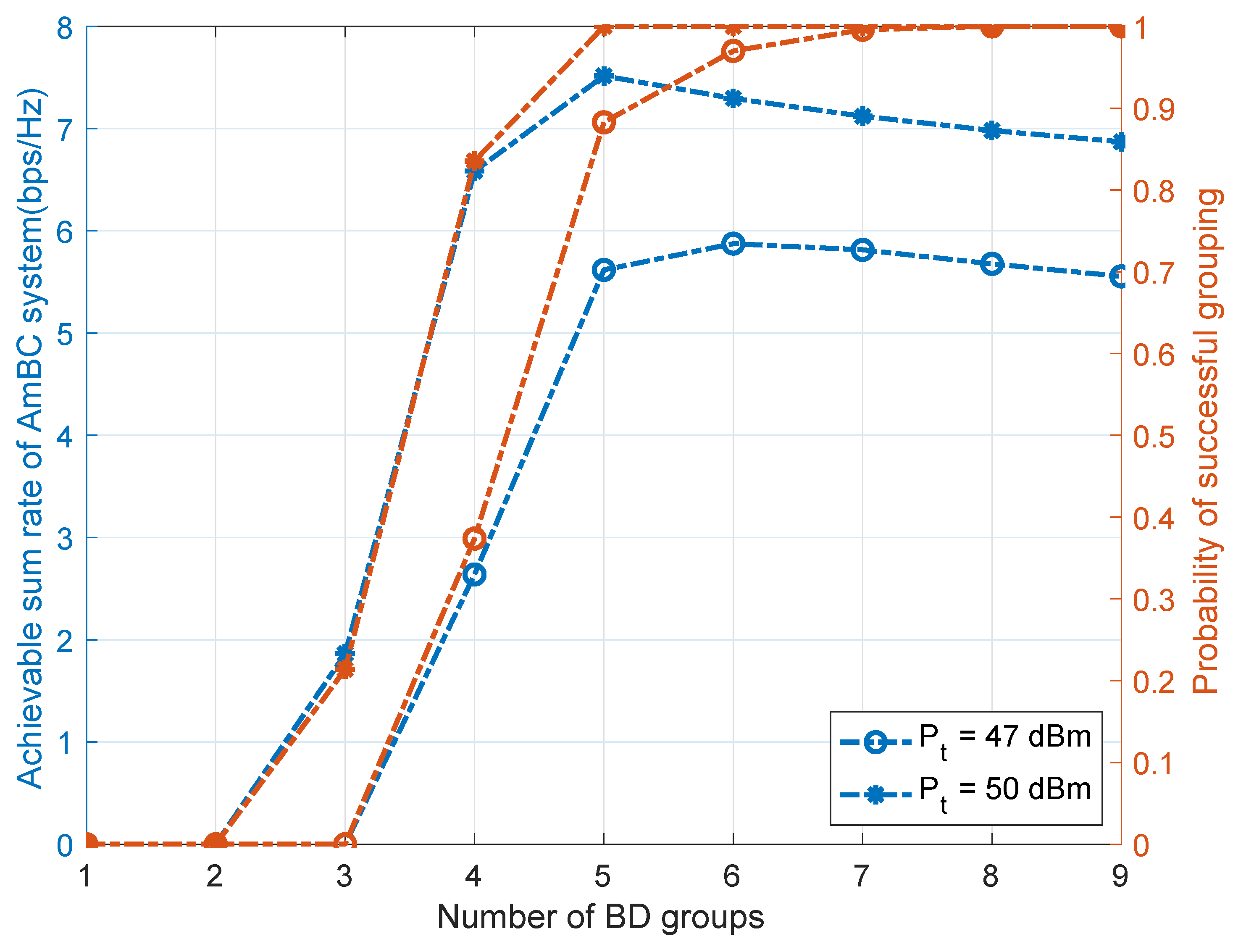
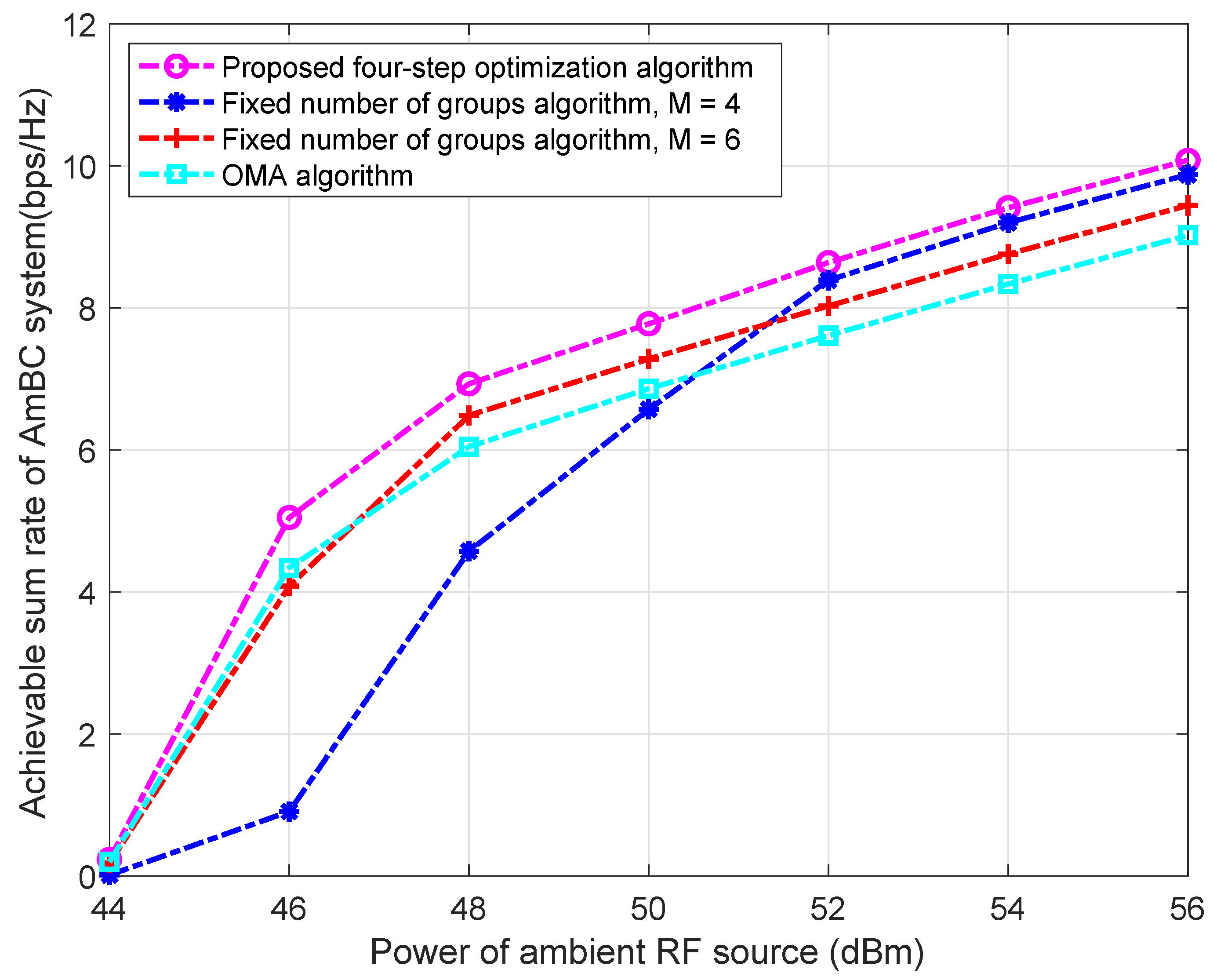
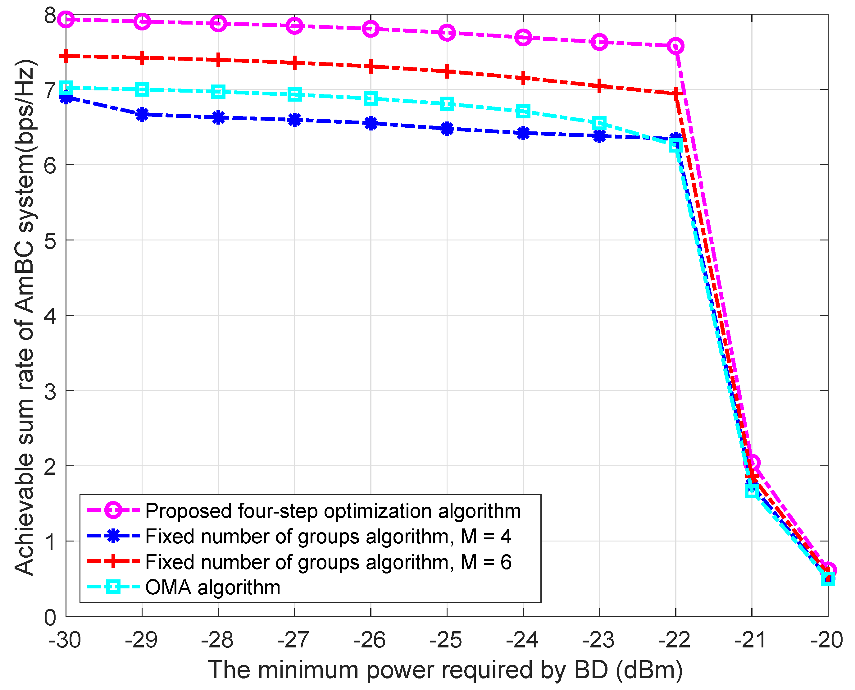
6.3. Proposed Algorithm

In this subsection, we will contrast the proposed algorithm with the two benchmark methods under various circumstances. The various circumstances mainly include the transmit power of the RF source, the SINR requirement of the RF signal, the SINR requirement of the BD signal, the minimum power required by BD, and the number of BDs.

As shown in Figure 3, we keep other variables unchanged and study the effect of the SINR requirement for decoding RF signal, i.e., ${\gamma }_t$, on the ASR of different algorithms. Obviously, the proposed four-step optimization algorithm is better than the other two algorithms. Figure 3 shows that changing the ${\gamma }_t$ for decoding the RF signal does not affect the performance of the above three algorithms when ${\gamma }_t$ is less than 50 dB. If the $SIN{R}_{m,t}$ obtained by (5) is much larger than ${\gamma }_t$, increasing the value of ${\gamma }_t$ does not have any effect on the optimal value of problem P1. In other words, the AmBC system does not affect the signal of the RF when ${\gamma }_t$ is less than 50 dB.

Next, we will analyze the impact of the SINR requirement of the BD signal, i.e., ${\gamma }_k$, on the ASR. As shown in Figure 4, the proposed algorithm is better than the other two algorithms. In particular, when ${\gamma }_k$ is bigger than 13 dBm, the proposed algorithm degenerates to the OMA algorithm, so the ASR of the two algorithms is the same. As ${\gamma }_k$ increases, the ASR of the fixed number of groups algorithm is even smaller than that of the OMA algorithm. The reasons for the above results are as follows. According to Equations (35) and (36), we can see that the lower bound of $a_n$ is related to ${\gamma }_k$. As ${\gamma }_k$ increases, the lower bound of $a_n$ keeps increasing. When the lower bound of $a_n$ exceeds the upper bound of $a_n$, the grouping strategy is failed, and a better grouping strategy should be found. For the fixed number of groups algorithm, as $a_n$ increases, more and more BDs fail to satisfy condition (35), thus leading to a lower probability of successful grouping. The reason why the ASR of $M=4$ is lower than that of $M=6$ is that the lower bound of $a_n$ is larger for $M=4$ compared to $M=6$, and therefore, the probability of successful grouping is lower under the same conditions.

The influence of the power of RF source, i.e., $P_t$, on the ASR is shown in Figure 5. The ASR increases with the increase in $P_t$; the proposed algorithm is better than the other two algorithms. This is because as the power of the RF source increases, the minimum number of groups is constantly decreasing. At the same time, when the BDs in the same group remain unchanged, as $P_t$ increases, ASR also increases. When $P_t=46$, the ASR of $M=4$ is smaller than that of $M=6$, but when $P_t=52$, the ASR of $M=6$ is larger than that of $M=4$. This is because the probability of successful grouping increases as $P_t$ increases, and the probability of successful grouping also increases as $P_t$ increases. Under the same conditions, the ASR of $M=4$ is greater than that of $M=6$ when both grouping strategies are successful. Therefore, although the probability of successful grouping of $M=6$ is not lower than that of $M=4$ when $P_t=52$, the ASR of $M=4$ is greater than that of $M=6$. The combination of the above two cases results in a situation where the ASR of $M=4$ is higher than the ASR of $M=6$ when $P_t=52$.

As shown in Figure 6, we analyze the impact of the number of BD on the ASR. It can be seen from Figure 6 that ASR does not change with the number of BDs, indicating that the proposed algorithm has the same stability as the OMA algorithm. However, the ASR of the proposed algorithm is better than that of the OMA algorithm. At the same time, we can also observe that for the fixed number of groups in an algorithm, the ASR increases first and then decreases with the increase in $K$. Increasing the number of BDs may increase ASR, but it may also cause algorithm failure. As the number of users increases, the probability of successful grouping gradually decreases. When the impact of algorithm failure on the system is less than the impact of part of the increase in ASR, the ASR of the system will show an upward trend, and vice versa, the average ASR of the system will show a downward trend.

As shown in Figure 7, we analyze the effect of the minimum power required by BD, i.e., $E_k$, on the ASR. It can be seen that when $E_k$ is less than −22 dBm, the ASR of the three algorithms slightly decreases but basically maintains a good performance, but when $E_k$ is greater than −22 dBm, the performance of all three algorithms decreases sharply. According to Equation (33), the upper bound of $a_n$ decreases with the increase in $E_k$. According to Equation (38), the upper bound of $a_n$ has an impact on the total ASR. However, when the value of $E_k$ does not affect the current grouping policy, the impact on ASR is relatively small. However, as $E_k$ continues to increase, the current grouping policy has no feasible domain, and the impact on ASR is huge. Finally, for large $E_k$, even in the case of OMA, some users are limited by constraints (2) that prevent them from activating the circuit of BD, while others are limited by constraints (8) that prevent them from decoding.

7. Conclusions

In this paper, we innovatively proposed the NOMA-assisted AmBC system. Compared with the OMA-assisted AmBC system, the proposed system can improve the ASR of the AmBC system. To maximize the ASR of the AmBC system, we formed a joint optimization problem in the BD grouping strategy including the number of BD groups and the BD allocation strategy, reflection coefficient, and decoding order. To simplify this problem, we transformed the above problem into a four-step optimization problem. Under the static grouping strategy, that is, when the number of BD groups and the BD allocation strategy are known, we give the optimal decoding order of BD and the closed-form solution of the reflection coefficient. Under the dynamic grouping strategy, the BD grouping strategy is divided into two steps: the BD group number strategy and the BD allocation strategy. Therefore, for a given number of BD groups, we propose a low-complexity BD allocation strategy based on the complexity–performance trade-off. The proposed algorithm can enhance the ASR of the AmBC system. However, the proposed algorithm also has some limitations in the AmBC system. Due to the uncontrollable power of the RF source, some BDs may not be able to obtain enough incident energy to drive the circuit. Even if the incident energy can drive the BD circuit, the receiving end still cannot obtain a good receiving SINR. Therefore, how to enhance the incident signal and reflected signal of the AmBC system is a problem that needs to be considered. A reconfigurable smart surface (RIS) can change the radio frequency environment, thereby changing the channel gain in the AmBC system. Therefore, we will introduce RIS in the future to enhance the NOMA-assisted AmBC system to further improve the ASR of the NOMA-assisted AmBC system.

References

1. van Huynh, N.; Hoang, D.T.; Lu, X.; Niyato, D.; Wang, P.; Kim, D.I. Ambient Backscatter Communications: A Contemporary Survey. Commun. Surv. Tutor. 2008, 20, 2889–2922. [Google Scholar] [CrossRef] [Green Version]
2. Kang, X.; Liang, Y.; Yang, J. Riding on the Primary: A New Spectrum Sharing Paradigm for Wireless-Powered IoT Devices. IEEE Trans. Wirel. Commun. 2018, 17, 6335–6347. [Google Scholar] [CrossRef] [Green Version]
3. Ishizaki, H.; Ikeda, H.; Yoshida, Y.; Maeda, T.; Kuroda, T.; Mizuno, M. A battery-less WiFi-BER modulated data transmitter with ambient radio-wave energy harvesting. In Proceedings of the 2011 Symposium on VLSI Circuits—Digest of Technical Papers, Kyoto, Japan, 15–17 June 2011; pp. 162–163. [Google Scholar]
4. Qian, J.; Gao, F.; Wang, G.; Jin, S.; Zhu, H. Noncoherent detections for ambient backscatter system. IEEE Trans. Wirel. Commun. 2017, 16, 1412–1422. [Google Scholar] [CrossRef]
5. Guo, H.; Long, R.; Liang, Y.-C. Cognitive Backscatter Network: A Spectrum Sharing Paradigm for Passive IoT. IEEE Wirel. Commun. Lett. 2019, 8, 1423–1426. [Google Scholar] [CrossRef]
6. Yang, G.; Zhang, Q.; Liang, Y.-C. Cooperative ambient backscatter communications for green Internet-of-Things. IEEE Internet Things J. 2018, 5, 1116–1130. [Google Scholar] [CrossRef] [Green Version]
7. Saad, W.; Bennis, M.; Chen, M. A vision of 6G wireless systems: Applications, trends, technologies, and open research problems. IEEE Netw. 2020, 34, 134–142. [Google Scholar] [CrossRef] [Green Version]
8. Zahid, N.; Sodhro, G.H.; Janjua, M.B.; Chachar, F.A.; Sodhro, A.H.; Abro, S.A.K. HARQ with chase-combining for bandwidth-efficient communication in MIMO wireless networks. In Proceedings of the 2018 International Conference on Computing, Mathematics and Engineering Technologies (iCoMET), Sukkur, Pakistan, 3–4 March 2018; pp. 1–6. [Google Scholar]
9. Ding, Z.; Lei, X.; Karagiannidis, G.K.; Schober, R.; Yuan, J.; Bhargava, V.K. A survey on non-orthogonal multiple access for 5G networks: Research challenges and future trends. IEEE J. Sel. Areas Commun. 2017, 35, 2181–2195. [Google Scholar] [CrossRef] [Green Version]
10. Dai, L.; Wang, B.; Yuan, Y.; Han, S.; Chih-lin, I.; Wang, Z. Non-orthogonal multiple access for 5G: Solutions, challenges, opportunities, and future research trends. IEEE Wirel. Commun. 2015, 53, 74–81. [Google Scholar] [CrossRef]
11. Li, D.; Liang, Y. Adaptive Ambient Backscatter Communication Systems with MRC. IEEE Trans. Veh. Technol. 2018, 67, 12352–12357. [Google Scholar] [CrossRef]
12. Zhang, J.; Zhu, L.; Xiao, Z.; Cao, X.; Wu, D.O.; Xia, X. Optimal and Sub-Optimal Uplink NOMA: Joint User Grouping, Decoding Order, and Power Control. IEEE Commun. Lett. 2020, 9, 254–257. [Google Scholar] [CrossRef]
13. Kimionis, J.; Bletsas, A.; Sahalos, J.N. Increased range bistaticscatter radio. IEEE Trans. Commun. 2014, 62, 1091–1104. [Google Scholar] [CrossRef]
14. Lu, X.; Niyato, D.; Jiang, H.; Kim, D.I.; Xiao, Y.; Han, Z. Ambient backscatter assisted wireless powered communications. IEEE Wirel. Commun. 2018, 25, 170–177. [Google Scholar] [CrossRef]
15. Duan, R.; Wang, X.; Yigitler, H.; Sheikh, M.U.; Jantti, R.; Han, Z. Ambient backscatter communications for future ultra-low-power machine type communications: Challenges, solutions, opportunities, and future research trends. IEEE Commun. Mag. 2020, 58, 42–47. [Google Scholar] [CrossRef]
16. Zhang, Q.; Zhang, L.; Liang, Y.-C.; Kam, P.-Y. Backscatter-NOMA: A symbiotic system of cellular and Internet-of-Things networks. IEEE Access 2019, 7, 20000–20013. [Google Scholar] [CrossRef]
17. Jameel, F.; Zeb, S.; Khan, W.U.; Hassan, S.A.; Chang, Z.; Liu, J. NOMA-enabled backscatter communications: Towards battery-free IoT networks. IEEE Internet Things Mag. 2020, 3, 95–101. [Google Scholar] [CrossRef]
18. Xu, Y.; Qin, Z.; Gui, G.; Gacanin, H.; Sari, H.; Adachi, F. Energy Efficiency Maximization in NOMA Enabled Backscatter Communications with QoS Guarantee. IEEE Wirel. Commun. Lett. 2021, 10, 353–357. [Google Scholar] [CrossRef]
19. Liao, Y.; Yang, G.; Liang, Y.-C. Resource allocation in NOMA- enhanced full-duplex symbiotic radio networks. IEEE Access 2020, 8, 22709–22720. [Google Scholar] [CrossRef]
20. Ihsan, A.; Chen, W.; Khan, W.U. Energy-Efficient Backscatter Aided Uplink NOMA Roadside Sensor Communications under Channel Estimation Errors. arXiv 2021, arXiv:2109.05341. [Google Scholar]
21. Khan, W.U.; Sidhu, G.A.S.; Li, X.; Kaleem, Z.; Liu, J. NOMA- enabled wireless powered backscatter communications for secure and green IoT networks. In Wireless-Powered Backscatter Communications for Internet of Things; Springer: Cham, Switzerland, 2021; pp. 103–131. [Google Scholar]
22. Le, C.-B.; Do, D.-T. Outage performance of backscatter NOMA re- laying systems equipping with multiple antennas. Electron. Lett. 2019, 55, 1066–1067. [Google Scholar] [CrossRef]
23. Lyu, B.; Guo, H.; Yang, Z.; Gui, G. The optimal control policy for RF-powered backscatter communication networks. IEEE Trans. Veh. Technol. 2018, 67, 2804–2808. [Google Scholar] [CrossRef]
24. Zhang, Q.; Zhang, L.; Liang, Y.; Kam, P.Y. Backscatter-NOMA: An integrated system of cellular and Internet-of-Things networks. In Proceedings of the ICC 2019—2019 IEEE International Conference on Communications (ICC), Shanghai, China, 20–24 May 2019; pp. 1–6. [Google Scholar]
25. Yang, G.; Xu, X.; Liang, Y. Resource Allocation in NOMA-Enhanced Backscatter Communication Networks for Wireless Powered IoT. IEEE Wirel. Commun. Lett. 2020, 9, 117–120. [Google Scholar] [CrossRef]
26. Khan, W.U.; Li, X.; Zeng, M.; Dobre, O.A. Backscatter-Enabled NOMA for Future 6G Systems: A New Optimization Framework Under Imperfect SIC. IEEE Commun. Lett. 2021, 25, 1669–1672. [Google Scholar] [CrossRef]
27. Li, X.; Zheng, Y.; Alshehri, M.D.; Hai, L.; Balasubramanian, V.; Zeng, M.; Nie, G. Cognitive AmBC-NOMA IoV-MTS Networks with IQI: Reliability and Security Analysis. IEEE Trans. Intell. Transp. Syst. 2021. [Google Scholar] [CrossRef]
28. Ahmed, M.; Khan, W.U.; Ihsan, A.; Li, X.; Li, J.; Tsiftsis, T.A. Backscatter Sensors Communication for 6G Low-powered NOMA-enabled IoT Networks under Imperfect SIC. arXiv 2021, arXiv:2109.12711. [Google Scholar]
29. Khan, W.U.; Javed, M.A.; Nguyen, T.N.; Khan, S.; Elhalawany, B.M. Energy-Efficient Resource Allocation for 6G Backscatter-Enabled NOMA IoV Networks. IEEE Trans. Intell. Transp. 2021. [Google Scholar] [CrossRef]
30. Khan, W.U.; Lagunas, E.; Mahmood, A.; Chatzinotas, S.; Ottersten, B. Integration of Backscatter Communication with Multi-cell NOMA: A Spectral Efficiency Optimization under Imperfect SIC. arXiv 2021, arXiv:2109.11509. [Google Scholar]
31. Zhuang, Y.; Li, X.; Ji, H.; Zhang, H.; Leung, V.C.M. Optimal Resource Allocation for RF-Powered Underlay Cognitive Radio Networks with Ambient Backscatter Communication. IEEE Trans. Veh. Technol. 2020, 69, 15216–15228. [Google Scholar] [CrossRef]
Figure 1. NOMA-assisted AmBC system.
Electronics 10 03061 g001
Figure 2. ASR vs. the number of BD groups.
Electronics 10 03061 g002
Figure 3. ASR vs. the SINR requirement for decoding RF signal.
Electronics 10 03061 g003
Figure 4. ASR vs. the SINR requirement decoding the BD signal.
Electronics 10 03061 g004
Figure 5. ASR vs. power of RF source.
Electronics 10 03061 g005
Figure 6. ASR vs. number of BDs.
Electronics 10 03061 g006
Figure 7. ASR vs. the minimum power required by the BD.
Electronics 10 03061 g007
Publisher’s Note: MDPI stays neutral with regard to jurisdictional claims in published maps and institutional affiliations.