Cost-Effective Data Aggregation Method for Smart Grid

Abstract

Finding a more efficient use of energy is an important problem that needs attention. Compared with the traditional power grid, a smart grid can monitor users’ electricity situation and electricity consumption instantly. However, it involves many problems of deploying network equipment. Consequently, it is vital to promote smart grids by collecting data from smart meters efficiently and keeping costs low. In this article, we propose a two-stage method of data collection for smart grids. The main contribution of this paper is to lower the number of data aggregation points (DAPs) so that the cost can be reduced. By using the K-means method, an entire smart grid can be divided into many smaller parts. In addition, the needs of transmitting and receiving data in the entire smart grid can be met by installing the least number of DAPs. Finally, the simulations show that the proposed two-stage method of data collection can use fewer DAPs to collect data than other methods which use one-stage methods, so the proposed scheme is more cost-effective.

1. Introduction

Because of the effects of climate change, more people have started focusing on the issues of energy conservation, carbon reduction, efficient energy use, and so on. In recent years, with the exuberant development of network, the concept of the smart grid is promoted vigorously. By promoting this, people hope to use and control energy efficiently; moreover, the traditional power grid can be replaced with smart grids. Compared with the traditional power grid, a smart grid can monitor users’ electricity situation and electricity consumption at a faster rate. Moreover, thanks to the availability of bi-directional communications, a smart grid can raise the efficiency of electricity and the reliability of the power grid. The infrastructure which supports bi-directional communication, called advanced metering infrastructure (AMI), was regarded as the fundamental structure of the smart grid [1]. To construct AMI, it is necessary to install smart meters (SMs) at home and all the electrical appliances at home need to be installed with sensors so that they can connect with SMs by a network. For example, in recent years, people often use wireless sensor networks which use Bluetooth, Wi-Fi and ZigBee to solve communication problems. Furthermore, users can monitor the electricity situations and transmit data using SMs to the control center instantly. As a result, the control center can immediately obtain the information on the electricity situations from each family, and users can also learn about the situations of every electrical appliance so that they can begin with allocating the utilization of electricity.

According to Greentech Media (GTM) Research, a smart grid can be divided into a power layer, a communications layer, and a smart grid application layer [2]. Besides, according to the communication range, AMI can be divided into three categories which are home area network (HAN), neighborhood area network (NAN), and wide area network (WAN). HAN contains SMs and other smart devices and often uses lower-cost communication techniques, such as Wi-Fi, ZigBee, PLC, Z Wave, and so on. NAN is between HAN and WAN. In NAN, the data from HAN will be collected and then be transmitted to WAN. Because of the need to handle bigger data in NAN, it uses wired networks, such as PLC, optical networks, or wireless networks, which have high data rates such as WiMAX. As for WAN, it connects several NANs and transmits data to the control center. In WAN, long-range communication techniques are often used, such as 3G, LTE, and LoRa.

In the smart grid system, when a great number of SMs transmit data at the same time, network congestion or collision will happen and even delay the entire system. As a result, communication quality is quite important for the smart grid. Researchers have proposed schemes to reduce delay in WAN [3,4,5]. A method was proposed to reduce delay in NAN by using the concept of data aggregation and defining a role, called data aggregation point (DAP), to receive all data from SMs [6]. However, choosing proper positions to install DAPs and be able to reduce delay at the same time is an important issue. We usually use a high-speed wired network to transmit data from DAPs to the control center, so it needs extra cost to install DAPs. Therefore, it is important to use a smaller number of DAPs [7,8]. In [9], applications of different optimization techniques are summarized. In [10], the methods which can reduce the cost of DAP in wired networks and wireless networks were proposed, while in [11], a cost-effective method to install DAP by using a utility pole was proposed. In [12], a heuristic algorithm using K-means was proposed to split the original set covering problem (SCP) into smaller ones that are optimally solved. Authors in [13] have formulated a constrained optimization problem, called cost minimization DAP placement (CMDP) to minimize DAP installation cost while satisfying communication QoS requirements. Because CMDP is proven NP-hard, a heuristic algorithm based on K-means was proposed to produce sub-optimal solution in reasonable time. In [14], a heuristic three-phase algorithm was presented for the optimal DAP placement in a multi-hop routing scenario, where SMs can serve as small relay devices so that communications among SMs can be leveraged to reduce the overall communication cost. K-means is a popular clustering algorithm that has advantages of high speed, but it suffers from the problem of local optimal. In [15], a clustering algorithm based on K-medoids was proposed. Although the mean square error for K-medoids is lesser than K-means, K-medoids is lacking in performance [16]. Owing to a bad choice of initial centroid locations and trapping into the local optimum easily, many articles have proposed to improve K-means by the particle swarm optimization (PSO) algorithm [17,18,19,20,21].

The aim of this paper is to reduce the number of DAPs. A role called cluster head (CH) is added to collect data from SMs and then transmit it to DAPs. We propose a new cluster algorithm to solve the problems of installing DAPs and choosing CHs. First, we divided SMs into several groups by using clustering and subsequently selected proper SMs from every cluster to be CH. In every cluster, all SMs could transmit data to DAPs through CHs.

The remainder of this paper is organized as follows. Section 2 presents the signal model. Section 3 describes the proposed algorithm. Section 4 illustrates the evaluation results. Finally, Section 5 draws the main conclusions.

2. Signal Model

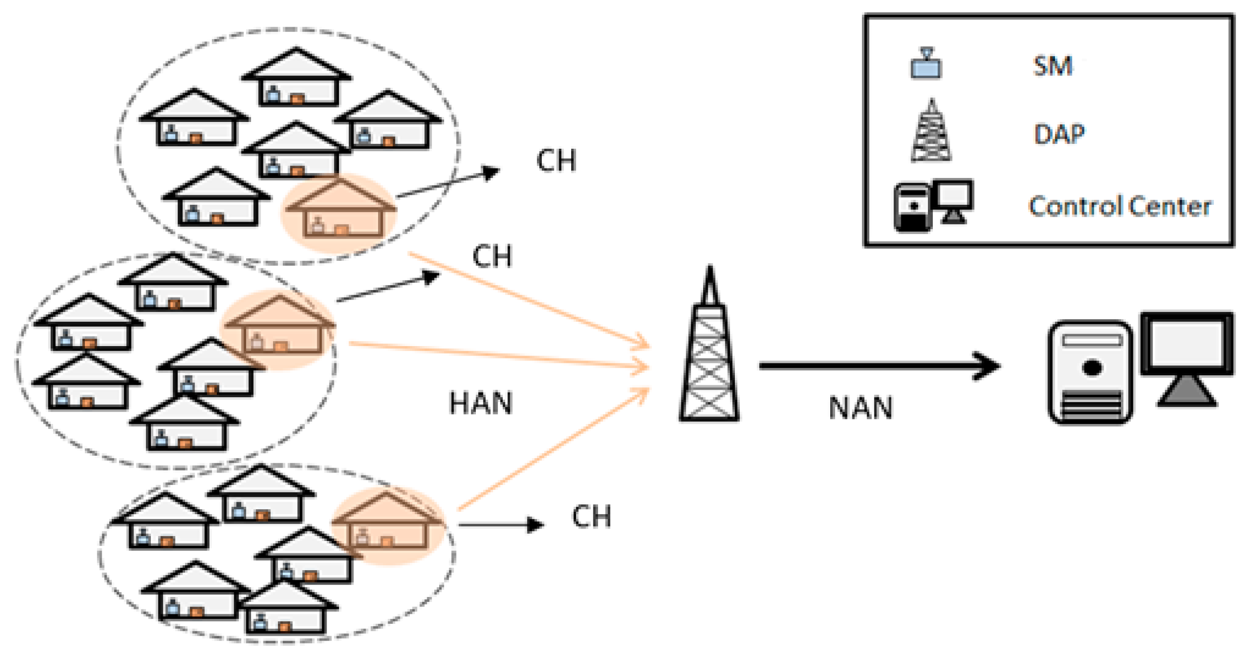
Here, a smart grid is divided into four categories, including SM, CH, DAP, and control center. Their main functions, as shown in Figure 1, are:

• SM: SM is installed in every home and the main function is to monitor the electricity situations in every family.
• CH: CH is a SM that is chosen from every cluster. Its main function is to collect data from all SMs in every cluster and transmit it to DAP.
• DAP: the main function of DAP is to collect data from CHs and then transmit it to the control center.
• Control center: the control center is used to receive data from DAPs and monitor the entire smart grid.

As shown in Figure 1, every house represents a family and has an SM in every house. First, we chose proper positions to install DAPs and then divided SMs into several clusters. In any area, SMs were divided into three clusters. Then, a proper SM was chosen to be a CH in every cluster. In this paper, we focus on the problems such as the transmission of data from SMs to CHs and CHs to DAPs. Our goal is to use the least number of DAPs and an optimal number of CHs.

The required signal-to-noise ratio (SNR) when CHs receive data from SMs, and DAPs receive data from CHs can be expressed as:

$${\mathsf{\gamma }}_{SM,CH,DAP}=\frac{P_t\times FSPL}{\sigma }$$

(1)

where $P_t$ is the transmission power, $FSPL$ is free-space path loss. The $FSPL$ in dB can be expressed as:

$$FSPL=10\times {\log }_{10}({(\frac{4\pi \times d_{snr}\times f}{c})}^2)$$

(2)

where $f$ is frequency, $c$ is the speed of light, and $d_{snr}$ is the threshold for distance. However, the supposed environment is not in free space, so the received signal power and the distance are nth power fading. Different values of n are presented in

Table 1. Path loss exponent in various environment.

Environments	Path Attenuation Index (n)
Free space	2
Metropolitan area	3~5
Building	4~6
Factory	2~3

. In this paper, the value of n is considered as 3, so the function can be rewritten as:

$$FSPL=20{\log }_{10}\left(f\right)+20{\log }_{10}\left(\frac{4\pi }{c}\right)+30{\log }_{10}\left(d_{snr}\right)$$

(3)

Besides, $\sigma$ is the thermal noise power in Watts which can be calculated by the formula as:

$$\sigma =K·T·B$$

(4)

where K is Boltzmann constant (at about 1.38 $\times {10}^{-23}$); and T is the temperature in degree K (°K). Because $\mathsf{\gamma }$ is the least SNR, ${\mathsf{\gamma }}_{SM,CH,DAP}$ should be larger than or equal to $\mathsf{\gamma }$. As a result, the SNR threshold is determined as follows:

$${\mathsf{\gamma }}_{SM,CH,DAP}\ge \mathsf{\gamma }$$

(5)

At last, the corresponding $d_{snr}$ in different SNR can be determined by Equations (1), (3), and (5). According to [13] and (4), assuming that packet error probability (E) is 0.01, packet length (L) is 1800 bits, bit per second (R) is 2 Mbps and bandwidth (B) is 1 MHz. In this case, the $\mathsf{\gamma }$ was estimated to be about 46 dB. Because $\mathsf{\gamma }$ is the least SNR, the ${\mathsf{\gamma }}_{SM,CH,DAP}$ must be large or equal to $\mathsf{\gamma }$. For example, giving n = 3, $P_t$ = 30 dBm, T = 298.15 °K (about 25 °C), f = 1 GHz, and c is 3 $\times {10}^5$ km, the $d_{snr}$ was measured to be about 1.53 km while $\mathsf{\gamma }$ is 46 dB.

3. Two-Stage Clustering Algorithm

In this section, the proposed scheme is described in detail. We aimed to aggregate data efficiently and reduce network delay by using the least number of DAPs and the optimal number of CHs. Using K-means to cluster SMs, it just groups SMs into several clusters and searches for the centroid in each cluster. However, it does not consider whether some SMs is too far from the DAP or not. When wireless communication techniques are used to transmit data, there are different distance restrictions due to transmission power and channel environments. Thus, a distance threshold $\left(d_{snr}\right)$ is added to constrict the farthest distance of SMs to CHs and CHs to DAPs. In this paper, we assumed that the $d_{snr}$ of SMs to CHs and CHs to DAPs were the same.

In smart grids, how to choose the number of DAPs and the locations to install DAPs is a non-deterministic polynomial (NP) problem [13]. To reduce the complexity, in this work it is used the K-means algorithm to partition SMs into several smaller parts.

For the K-means algorithm, Euclidean sum of squares is defined as fitness function:

$$Fitfunction={\displaystyle \sum }_{i=1}^N{\left[\left(X_i-Cen\left(j\right)\right)\right]}^2$$

(6)

where $X_i$ is the coordinate of ith SM and $Cen\left(j\right)$ is the initial centroids when dividing into j clusters. We expected to find the centroid, which means that the sum of squared shortest distances of all SMs to the centroid was minimized.

A two-stage clustering algorithm to determine the least number of DAPs and an optimal number of CHs is proposed. At the first stage, the required amount of DAPs, denoted by K, is determined and a single DAP (i.e., K = 1) is tested at the beginning. At this stage, all SMs were divided into K clusters, and let K DAPs be placed at the K centroids. At the second stage, in each of the K clusters, SMs were divided into smaller sub-clusters, while a SM was chosen as the CH in each sub-cluster, until the distance from all SMs to the CH in each sub-cluster and all CHs to the DAP in each of the K clusters were shorter than the distance threshold $\left(d_{snr}\right)$. The proposed clustering algorithm is described as below:

(1)

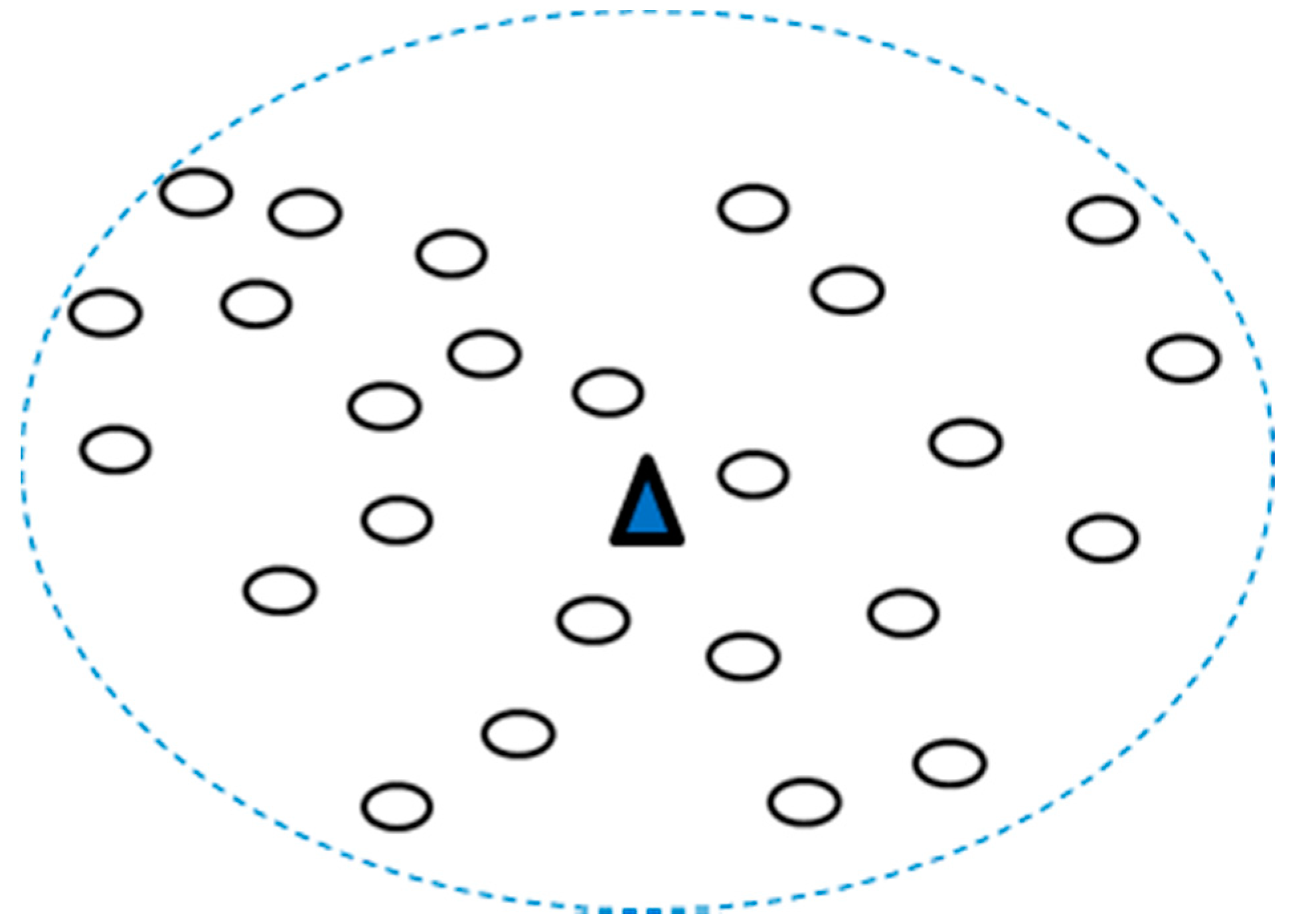
Set K = 1, regard all SMs as one cluster.

(2)

Use the K-means algorithm to find out the least fitness as well as the optimal corresponding K centroids and install a DAP in each centroid, as shown in Figure 2.

(3)

Clustering all SMs covered in each DAP.

• When the clustering result met the distance threshold ($d_{snr}$), the optimal number of clusters is determined. Therefore, the algorithm is stopped.
• If no candidate CH for any SM can meet the distance threshold, SMs are continually grouped into smaller clusters until all SMs become CHs. As a result, one DAP (K = K + 1) is added and return to Step (2).

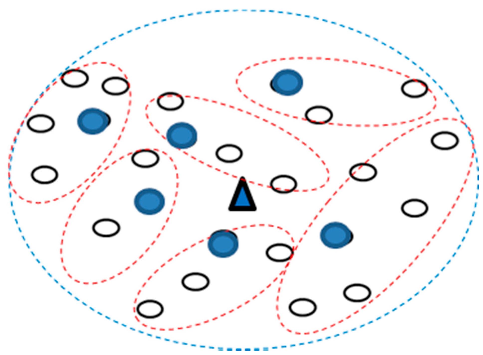
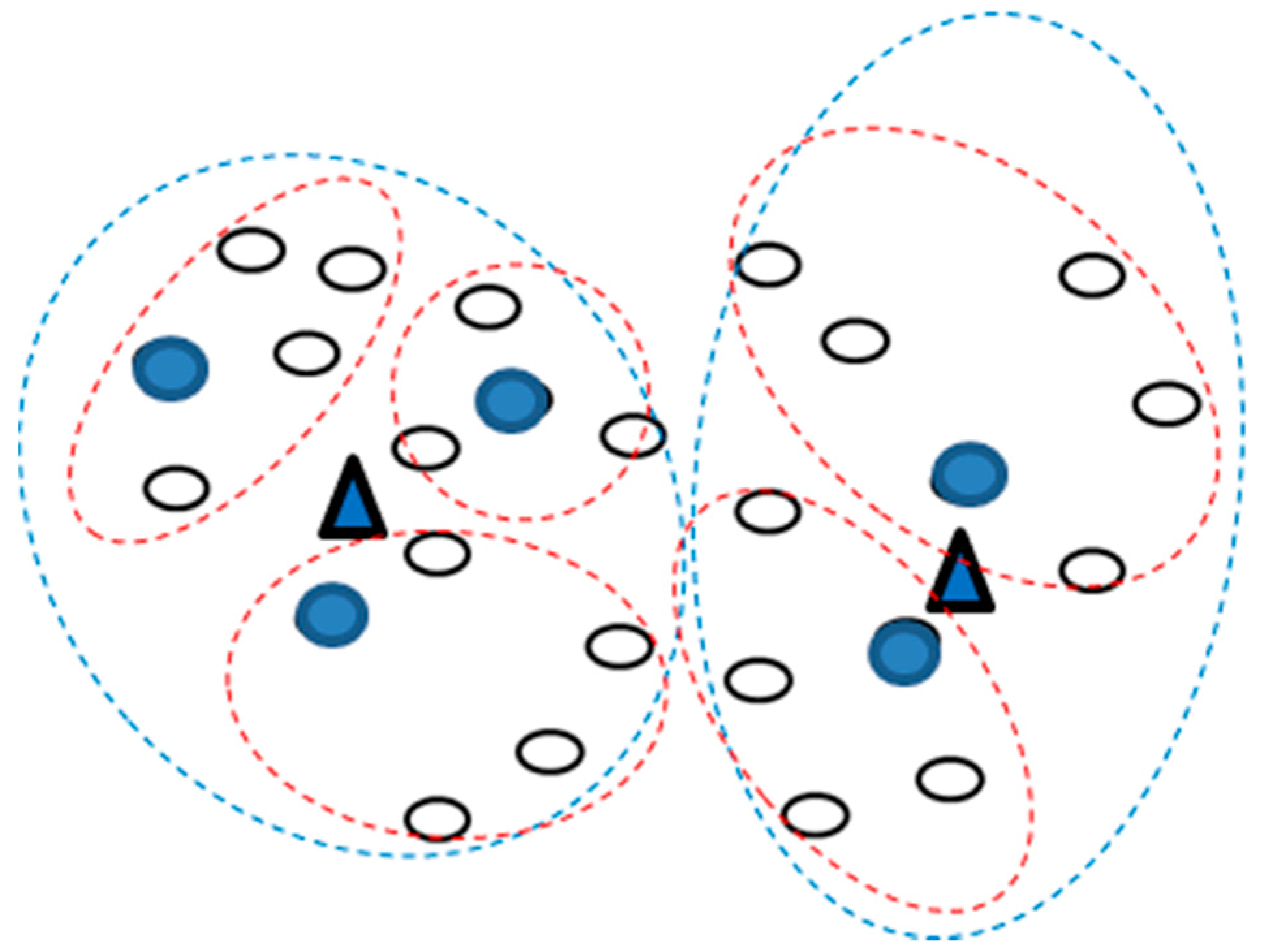
Finally, the number of DAPs needed to be installed in this area and the number of CHs needed in every DAP are determined. As shown in Figure 3, the optimal number of clusters was 6, so 6 CHs (blue dots in the figure) could be obtained. However, on adding the other one DAP, as in Figure 2 (i.e., K = 2), the obtained clustering result is shown in Figure 4.

The K-means algorithm can also determine the centroid in every cluster, and therefore, we choose the SM closest to centroid as CH in every cluster because a centroid is a point where the sum of squares of the shortest distance to every SM is minimum. Although SMs are not mobile devices, new SMs might be added to a cluster, and other SMs might be removed from a cluster. As a result, if that happens, the cluster should be reconfigured.

When data are transmitted from transmitter to receiver, they must be affected by the environment or by passing too many hops so that there may be a delay. Delay may be of two types, propagation delay, and media access delay, as described below:

(1)

Propagation delay: this delay time is the duration when a packet transmits from transmitter to receiver. This time is affected by the distance, and the farther the distance is, the higher the delay is. Assuming that the distance between transmitter and receiver is $d$ and transmission rate is $v$, so, the time it costs is $d/v$. However, because the speed of transmission equals to speed of light, the delay caused by propagation delay is very low.

(2)

Media access delay: this delay time is the duration when a packet transmits successfully. If a packet transmits unsuccessfully, it is retransmitted until it is successful. Suppose that the media access delay $D_m$ is a packet that transmits once successfully and if a packet transmits unsuccessfully for the first time, then the delay time when it transmits for the second time is $2D_m.$ Hence, if this packet transmits successfully at the nth time, the delay time is $n\times D_m$. As a result, the greater number of times the packet is retransmitted, the higher the delay is. The media access delay is the primary delay when a packet transmits.

The proposed two-stage clustering algorithm utilizes CH to receive data from SMs and transmit it to DAP, so it can reduce the number of DAPs with the same distance threshold. Compared with the method presented in [13], the proposed method causes a greater delay because data are transmitted through more hops. Suppose $D$ is the total delay when a packet transmits from transmitter to receiver, $D_p$ is propagation delay, $D_m$ is media access delay, assuming $D_p+D_m\cong D_m$, where $D_p$ is significantly short and can be ignored. Here, $D$ can be calculated by the packet error rate (PER). Thus, $D$ can be expressed as:

$$D=\left(1-P\right)\times D_m+P\times \left(1-P\right)\times 2D_m+P^2\times \left(1-P\right)\times 3D_m+\dots$$

(7)

where $P$ is the PER. Then, Equation (7) can be rewritten by multiplying P, it can be expressed as:

$$P\times D=P\times \left(1-P\right)\times D_m+P^2\times \left(1-P\right)\times 2D_m+P^3\times \left(1-P\right)\times 3D_m+\dots$$

(8)

Subtracting Equation (7) from (8) and we can obtain:

$$\left(1-P\right)\times D=\left(1-P\right)\times D_m+P\times \left(1-P\right)\times D_m+P^2\times \left(1-P\right)\times D_m+\dots$$

(9)

Finally, Equation (9) can be simplified as below:

$$\begin{array}{cc}D& =D_m{\displaystyle {\displaystyle \sum }_{i=0}^{\infty }}{\left(P\right)}^i\hfill \\ & =\frac{D_m}{1-P}\hfill \end{array}$$

(10)

In the proposed method, SMs will transmit data to CHs, and then CHs will transmit these data to DAPs. Assuming that $P_{ch}$ and $P_{dap}$ are the PER which are when SMs transmit data to CH and the PER when CHs transmit data to DAP, respectively. Finally, we can calculate the delay by PER. Suppose $\frac{D_m}{1-P_{ch}}$ and $\frac{D_m}{1-P_{dap}}$ are expressed as the delay when SMs transmit data through two hops. So, the total delay can be expressed as:

$$D=\frac{D_m}{1-P_{dap}}+\frac{D_m}{1-P_{ch}}$$

(11)

4. Evaluation Results

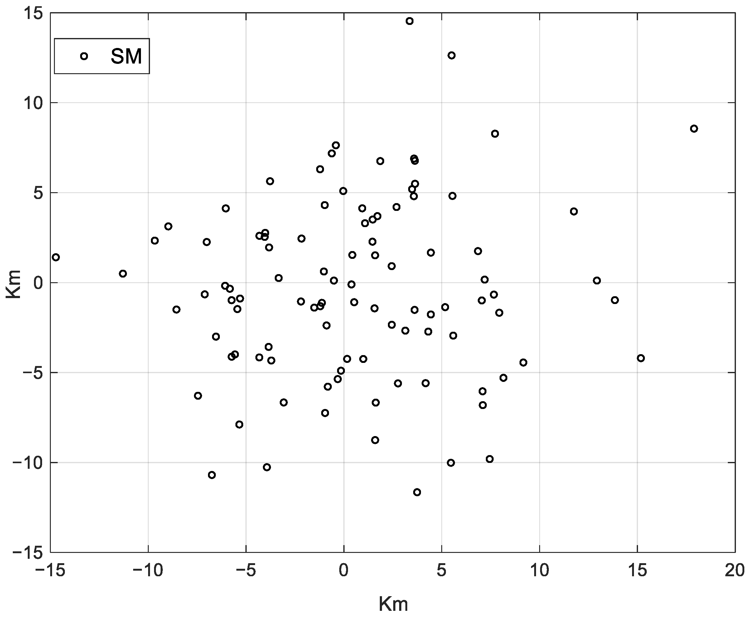
To evaluate the performance in the delay time (D) and required amount of DAPs, we compared our two-stage data aggregation method with the method presented in [13]. In this paper, MATLAB is used for simulation. To verify that our proposed scheme can be applied to various distributions of SMs, the command ‘randn’ in MATLAB is used to generate locations for SMs, which are shown as a normal distribution. As a result, most SMs concentrated in the middle area. Figure 5 shows the simulation result of SMs’ distribution. A total of 100 SMs are produced, which were randomly distributed in $40\times 40{\mathrm{km}}^2$ area. Most SMs were concentrated in the middle and were only seldom SMs scattered in faraway areas.

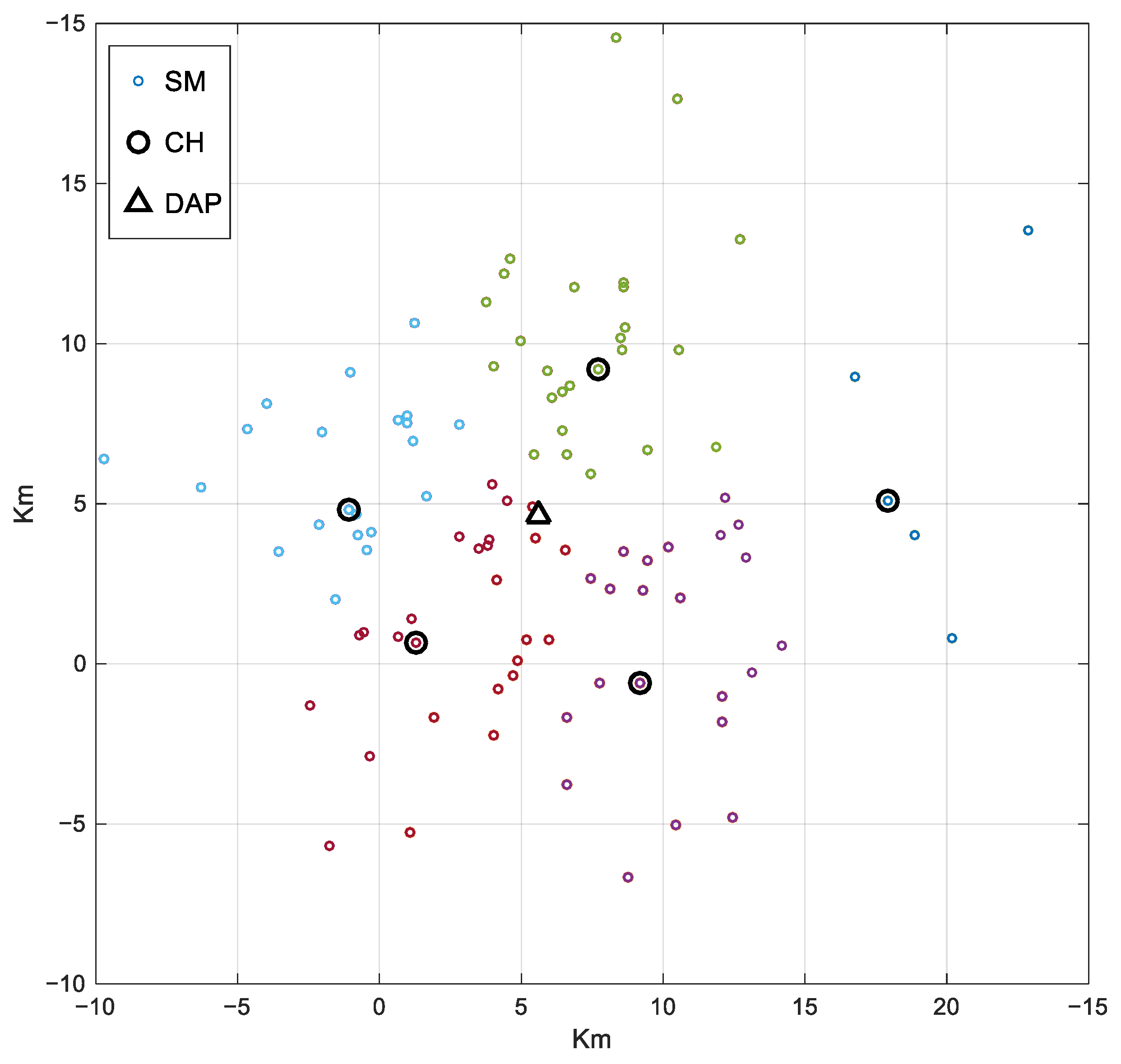
Assuming PER to be 0.01, packet size L of 1800 bits, transmission rate R of 2 Mbps, bandwidth B of 1 MHz, the SNR threshold $\mathsf{\gamma }$ was 46 dB, and distance threshold $d_{snr}$ was 7.1 km. Figure 6 shows the result of clustering. The triangle icon is expressed as DAP, the bigger circle icon is expressed as CH in every cluster, and the SMs which have different colors are expressed the SMs belong to different clusters.

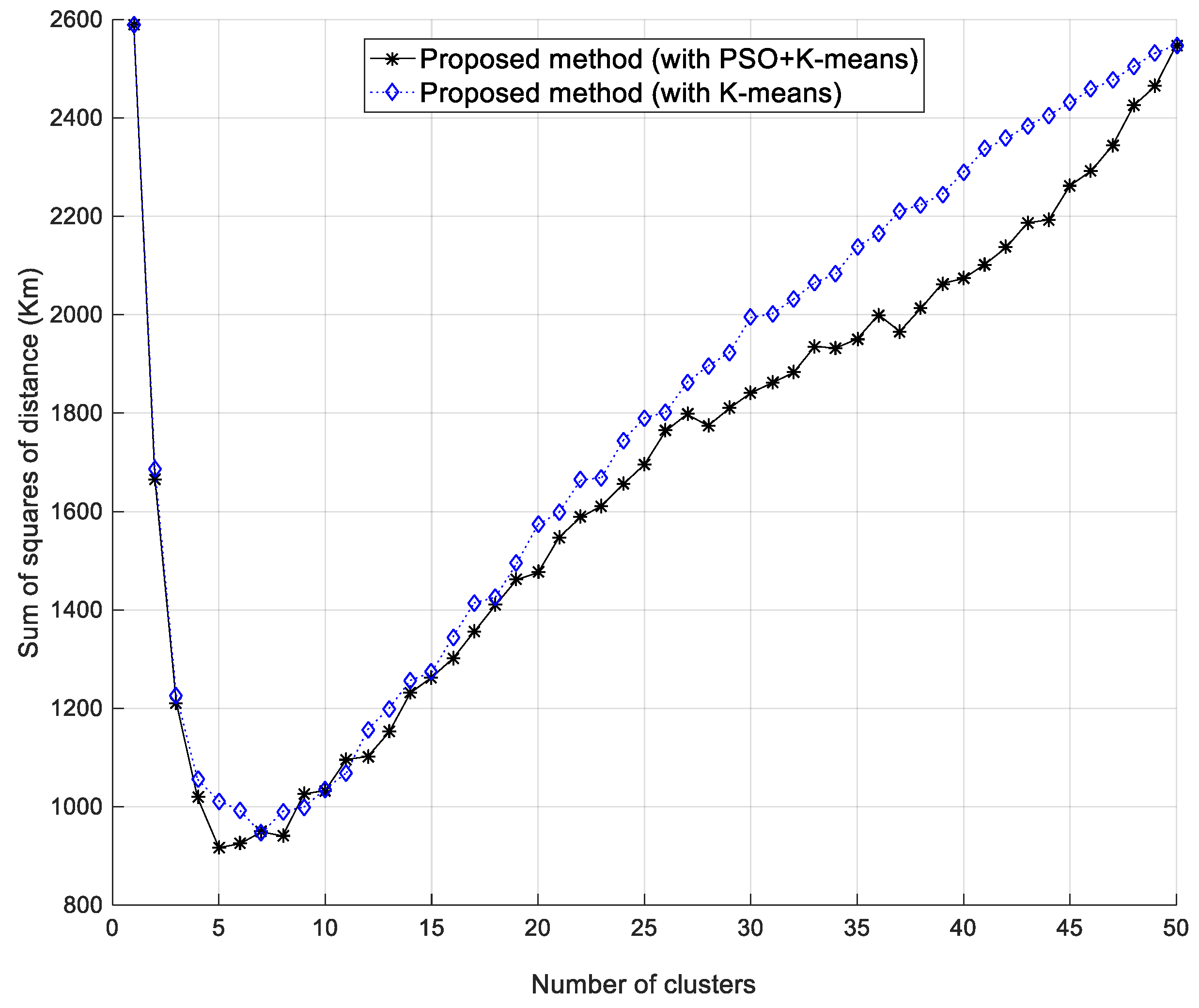
Because K-means suffers from the problem of local optimal, the combination of PSO and K-means is used to improve the K-means clustering problem [18]. Figure 7 shows the comparison of the sum of the squares of the distance between K-means and K-means improved by PSO, denoted as “PSO + K-means”. It has a lower sum of the distance while K-means is improved by PSO. A lower sum of the distance means that the PSO + K-means scheme yields a better clustering result.

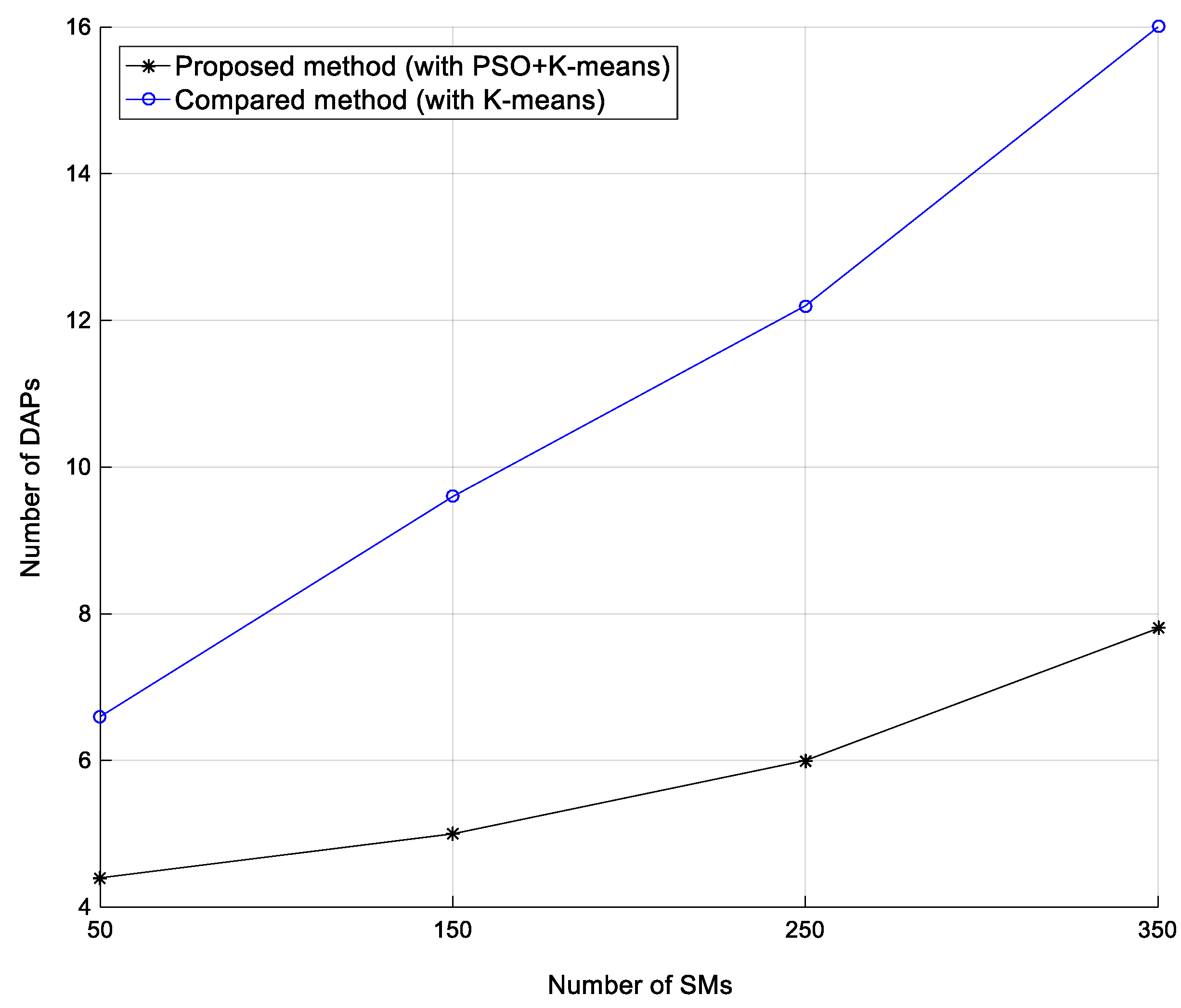
The comparison of the required amount of DAP for different numbers of SMs is shown in Figure 8. The dotted line is the compared, one-stage method presented earlier [13]. In the one-stage method, SMs transmit data to DAPs directly. When the distance between SM and DAP is longer than the distance threshold ($d_{snr}$), it will add one DAP and restart clustering until the distance between each SM and a DAP is shorter than the distance threshold. As shown in Figure 8, the horizontal axis is expressed as the number of SMs, from 50 to 350, and the vertical axis is expressed as the amount of DAP. The distance threshold is 7.1 km. With the increase in the number of SMs, the amount of DAP necessary to install also increase. Obviously, the amount of DAP necessary in this study was less than that in the earlier proposed method [13].

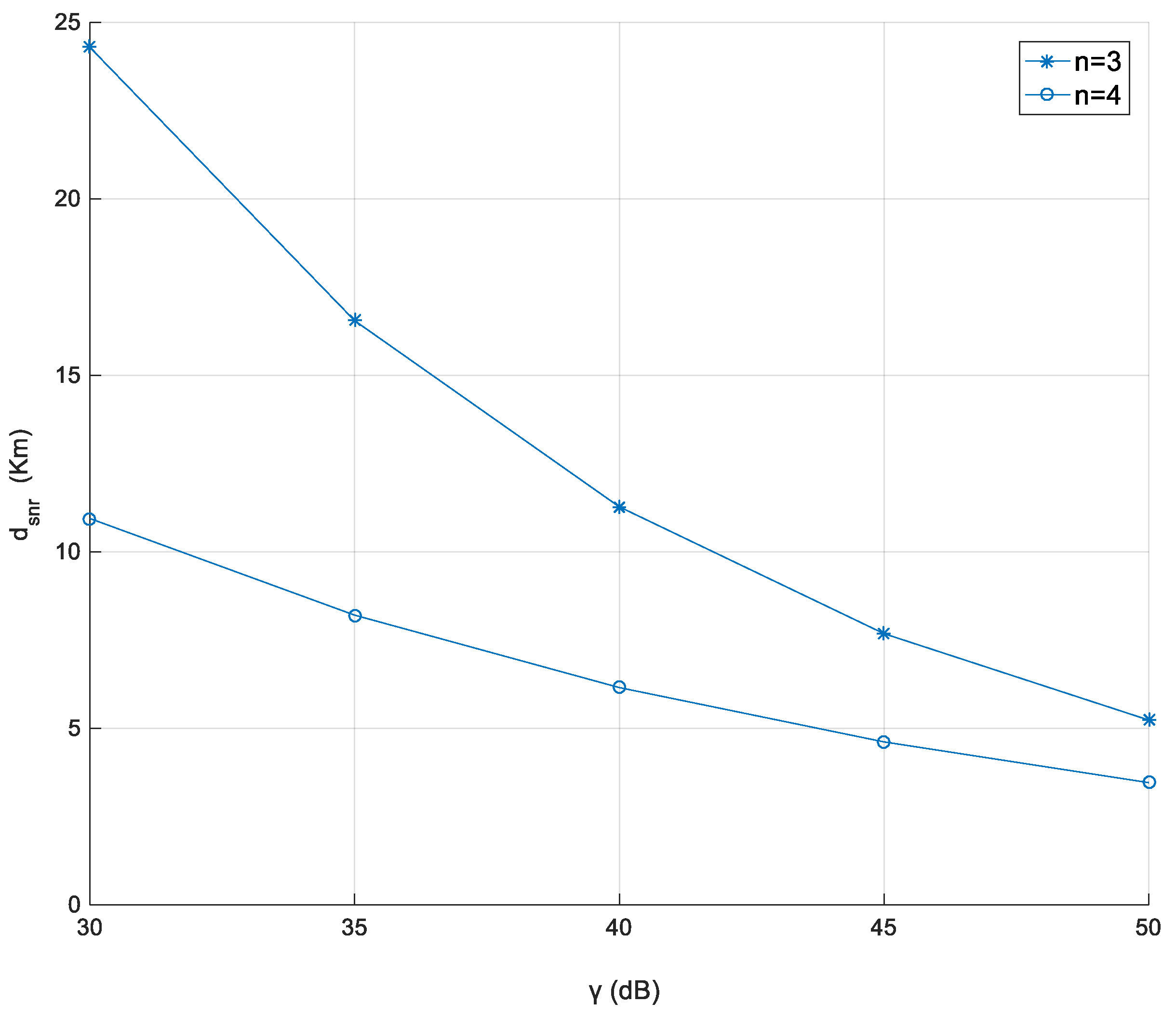
Figure 9 shows the relationship of distance threshold ($d_{snr})$ according to different SNR thresholds ($\mathsf{\gamma }$). Here, $\mathsf{\gamma }$ is about 30 dB where the corresponding $d_{snr}$ is about 24 km; $\mathsf{\gamma }$ is about 40 dB where the corresponding $d_{snr}$ is about 11 km; and when $\mathsf{\gamma }$ is about 50 dB, the corresponding $d_{snr}$ is about 5 km. This is because the received power is lost when the distance increases. As a result, to maintain higher SNR, the distance is not too far.

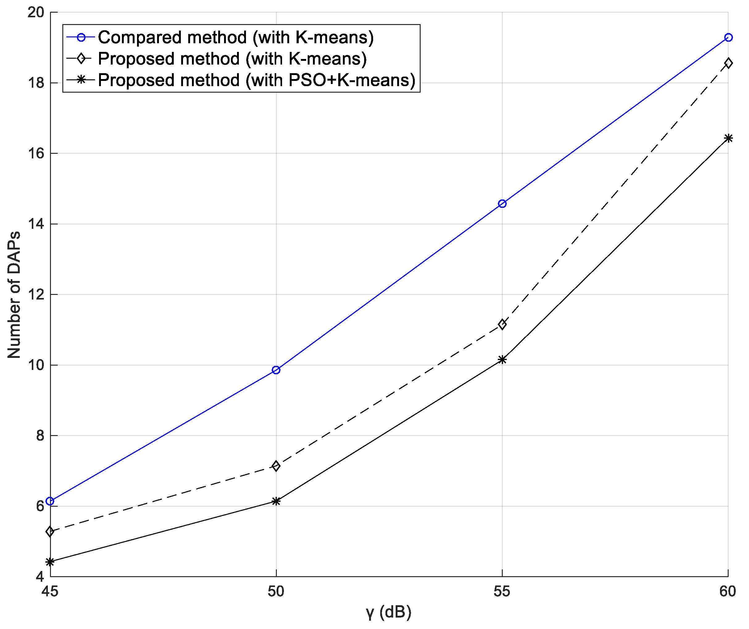
Figure 10 shows the required number of DAPs in different $\mathsf{\gamma }$. In this simulation, 100 SMs are used, and the value of $\mathsf{\gamma }$ was from 45 dB to 60 dB. According to this figure, when the value of $\mathsf{\gamma }$ raises, the required number of DAPs also increases. According to Figure 9, the higher the $\mathsf{\gamma }$ is, the smaller is the $d_{snr}$. As a result, when $d_{snr}$ is smaller, the distance between every DAP and CHs as well as the distance between every CH and SMs becomes shorter. While $d_{snr}$ becomes smaller, the range every DAP can cover is also reduced and the required number of DAPs increases. The dotted line is the method proposed by the earlier study [13] and the solid line represents our method. The required number of DAPs with the proposed method was fewer than that in the earlier proposed method [13].

The average delay is calculated by Equation (11). The packet error rate can be calculated by bit error rate (BER), as below:

$$P=1-{\left(1-b\right)}^L$$

(12)

where $b$ is BER; and L is the number of bits per packet. By using Formula (13) mentioned in [22], the BER can be calculated by a given SNR. In this paper, the SNR was calculated by Equations (1) and (3) with a known distance. Therefore, $P_{ch}$ was derived by the distance between an SM and its CH, and $P_{dap}$ was derived by the distance between a CH and its DAP.

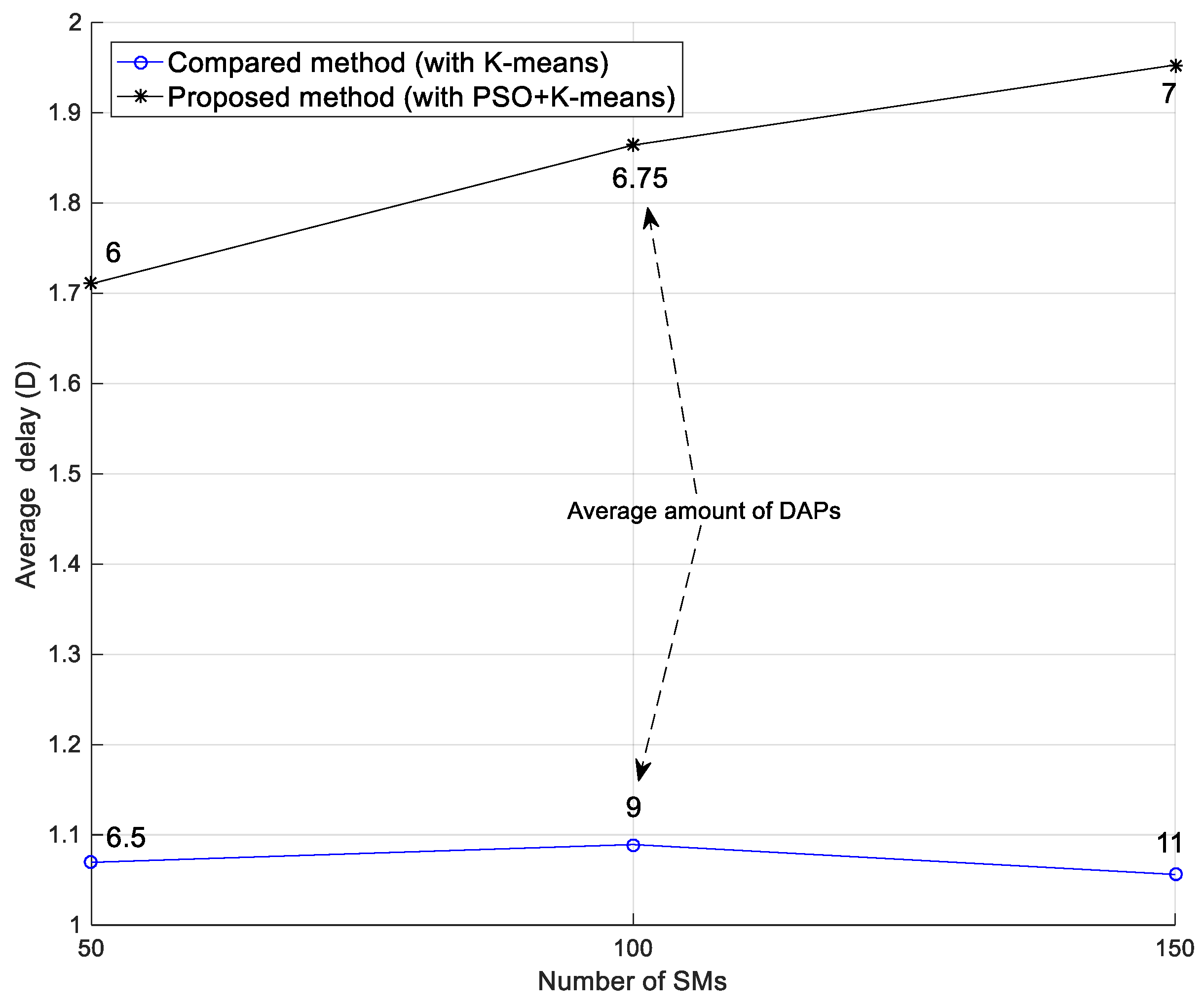
Figure 11 shows the comparison of delay with different numbers of SMs. The horizontal axis is the number of SMs, and the vertical axis represents the average delay. The average delay for the compared method and our proposed method was calculated using Equations (10) and (11), respectively. According to this figure, it is shown that the delay in the proposed method was higher than the compared method [13]. However, in 50 SMs, the average number of DAPs in the proposed method was 6, while that of the compared method is 6.5. Furthermore, when the number of SMs increased to 150, the average amount of DAPs in the proposed method was 7, and that of the compared method was 11. Therefore, it is concluded that although the delay in our proposed method is higher, the average number of DAPs is fewer than that of the compared scheme. Moreover, while the number of DAPs increased, the average delay with the compared method was lowered because the distance between every DAP and SMs was shortened.

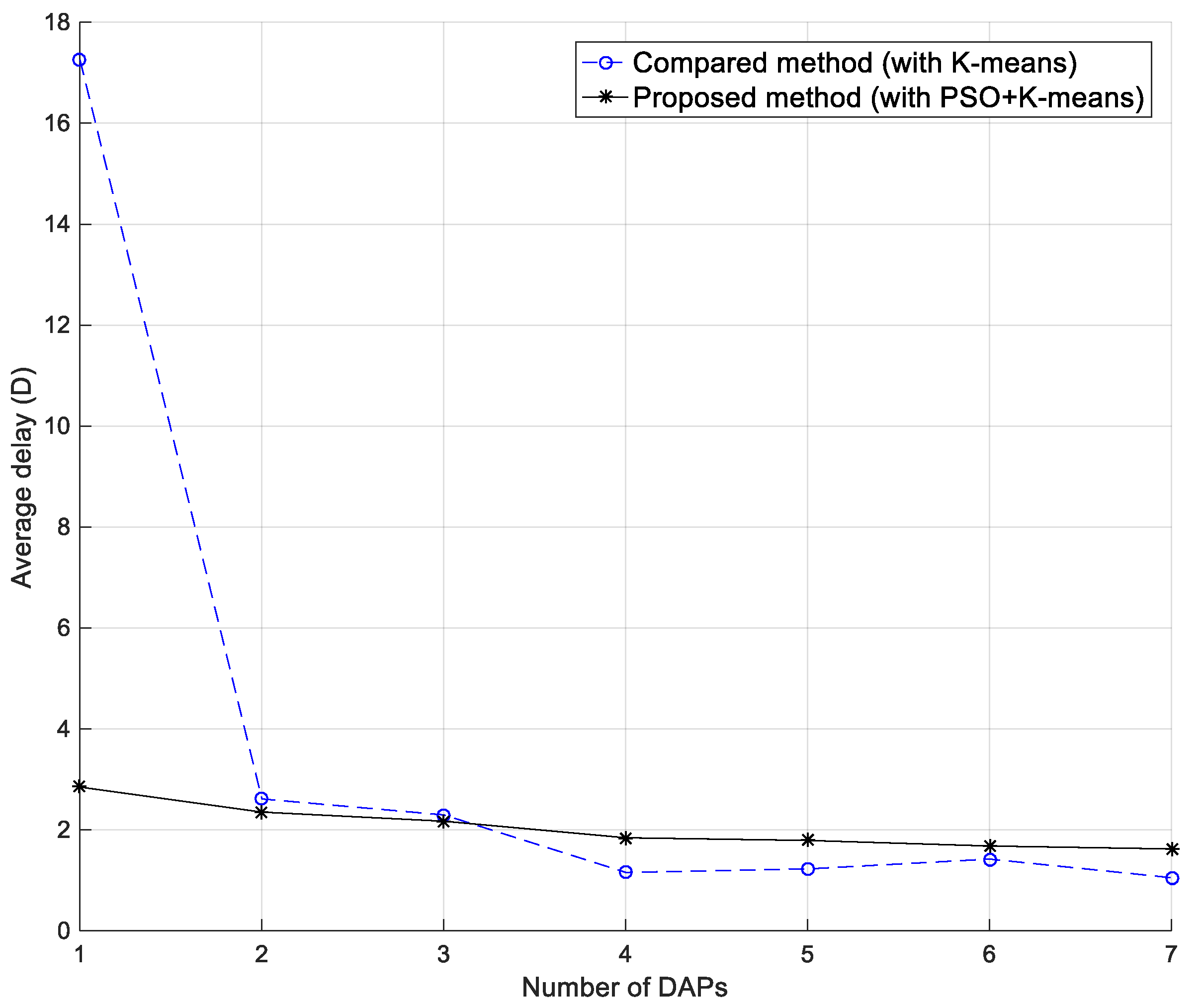
Figure 12 shows the relationship of average delay with our proposed method and the compared method [13] with the same number of DAPs, while 50 SMs are used. With a single DAP, the average delay with the compared method was much higher than that in our proposed method, because the compared method divides all SMs into one cluster. As a result, the average distance between the DAP and all SMs is longer than that in our proposed method. Significantly, the longer distance brings about a higher PER. As shown in Equation (10), the time delay depends on the PER. However, with the number of DAPs larger than three, the average delay was worse with our proposed method than the compared method. This may be because if the SMs in one area has good results of clustering, too many hops cause higher delay.

5. Conclusions

Owing to the high cost of installing a DAP, our aim was to use as few DAPs as possible. In this study, we used K-means clustering to divide SMs into several clusters and used a two-stage method to aggregate data. The proposed two-stage clustering algorithm utilizes CH to receive data from SMs and transmit it to DAP, so it can reduce the number of DAPs. However, because our method is with a two-stage mechanism, an SM needed two hops to transmit its data through a CH to a DAP. It may cause a greater delay because data are transmitted through two hops, but the per-hop delay is reduced because the transmission distance is shorter. To fairly compare average delay of our proposed scheme to the compared scheme, the delay time was formulated as Equations (10) and (11). As a result, the required number of DAPs with our proposed method was significantly fewer although the average delay with our proposed method was a little higher than that with the compared method. Thus, our proposed method is more cost-effective than the compared method.