An Efficient Indoor Positioning Method with the External Distance Variation for Wireless Networks

Abstract

This study strengthens the external distance variation for the indoor positioning performance. With the received signal strength (RSS) of the unknown node, a localization is performed to positioning its coordinates. The mean square error (MSE) of localization is deteriorated by the shadowing effect and the MSE depends on the location of reference nodes. Moreover, the minimum mean square error (MMSE) algorithm is also used with the RSS. The amount of variation in the distance between the reference point and the positioning node will also affect the accuracy. Therefore, this paper considers the distance between the reference point and the positioning node and also the distance variation between the reference points. MSE is used to estimate positioning performance and Monte Carlo is also used to simulate the average error of different shadowing and decay environments. When reference nodes have known distances, the distance is obtained separately and the estimated distances are identified by the MMSE method. In order to reduce the number of reference nodes and calculation cost, this paper uses adaptive reference node selection to improve the accuracy of positioning. Simulation results show that the external distance variation mechanism strengthens the indoor positioning performance. Moreover, this paper investigates the performance of several reference nodes (three, four, five, and six reference nodes) through 3D graphs to estimate the small range area. The differences are more clearly observed with fewer reference nodes and lower MSE. Finally, simulation results show that the MSE value of fixed three reference nodes is almost 100% better with external distance variation method compared to the random selected three reference nodes.

1. Introduction

In recent years, wireless networks are developed quickly and have been applied to many places such as hot spots, personal digital devices, and so forth [1,2]. The wireless network technology is also applied into the wireless personal area network (WPAN) that specializes in some devices of short-distance transmission and low power consumption such as Bluetooth, ZigBee, and so on [3,4,5]. However, the wireless networks have developed rapidly and become one of the hot research topics that indoor positioning technology is particularly important for. The applications of wireless network communication positioning are very mature and popular compared to the technology of global positioning system (GPS) [4,5]. The GPS technology uses satellites to provide three-dimensional positioning. GPS also provides accurate positioning in outdoor applications not suitable for indoor positioning.

The positioning technology normally has two different types that are distance-based (range-based) and non-distance-based (range-free-based) [6,7,8,9,10,11]. The distance-based method basically uses angle or distance information to estimate the positioning location. Most of the distances are measured through radio signals or ultrasonic waves, and the positioning procedure that can be performed without knowing the distance information. The distance-based positioning algorithm [12] has different methods to estimate the distance that are the time of arrival (ToA) method, the time difference of arrival (TDoA) method, the angle of arrival (AOA) method, and so on [13,14,15].

The received signal strength method (RSS) is used for distance estimation [16,17]. When estimating the distance, there is no need to add additional equipment, and there is no time synchronization problem. Therefore, substituting the power received by the unknown node into the attenuation model can find the distance. This paper uses the RSS to estimate the distance between the unknown location and the reference point. The accuracy of RSS positioning is greatly affected by the shadowing effect, and then the minimum mean square error (MMSE) algorithm is used for triangulation to locate the coordinates of unknown nodes. Because of the signal affected by different degrees of shadow fading, positioning error happens [18]. However, shadow fading can be modeled by a random variable of log-normal distribution with zero mean and the standard deviation σ = 3–8 dB [19]. In order to reduce the number of reference nodes and calculation cost, this paper uses an adaptive reference node selection to improve the accuracy of positioning.

Wireless communication is to use the electromagnetic wave as a conductive medium to communicate without going through a wired communication. Therefore, since the Second World War, wireless communication has been used in the military. The results of the application are valued and there is a lack of extensive communication standards. Therefore, the Institute of Electrical and Electronics Engineers (IEEE) formulated the first version of the standard called IEEE 802.11 for wireless local area networks in 1997, which redefines and modifies the media access control (MAC) layer and the physical (PHY) layer [20]. The two devices can be transmitted in a point-to-point (Ad Hoc) manner, or under the coordination of a base station (BS) or an access point (AP).

After the signal is sent from the transmitter, all path distances before reaching the receiver are called channels. If the signal is a radio signal, the propagation path is called a wireless channel. The factors caused propagation loss of radio signals during channel propagation can be roughly divided into two categories: the large-scale propagation model and the small-scale propagation model. The influencing factor of the large-scale propagation model is the change caused by the long distance or time of the signal in the transmission process. The small-scale propagation model analyzes the change of the signal in a short distance or a short period of time, and the change of the signal in a short distance and a short period of time may be affected by the movement of surrounding objects, such as the movement of a large vehicle or the movement of the mobile phone itself or caused by natural environments. Wireless telecommunication signals change very quickly in mobile communication, a very important factor affecting communication quality. This phenomenon is unavoidable and the radio wave part is still on the bottleneck of communication performance in the overall mobile communication system.

The factors affected by the signal strength of radio waves can be divided into three categories; the first category being the path loss [21], which is the main reason for the attenuation of radio wave signal strength. When a signal is sent by an antenna, its energy distribution is determined by the radio wave radiation. As the distance increases, the radio wave power per unit area decreases. The second category is the slow fading or shadowing. The main reason is that large-scale natural buildings exist on the earth’s surface. The former are hills or forests, and the latter are residential buildings. Districts or large factories in wireless communication systems will cause interference effects on radio waves. The radio wave signal attenuation of these large-scale buildings is relatively unchanged with time. The strength of the wireless telecommunication signal will be inversely attenuated with the fourth or fifth power of the actual distance. The third category is the fast fading referred to a situation where the signal presents a large change in a short period of time. It may be affected by the movement of the receiving point or surrounding objects. The latter is a situation caused by an instantaneous change in the natural environment. A modelized description of radio wave transmission is helpful for system operators to plan and build base stations. Many papers have proposed quite a lot of channel models, which can be roughly divided into the following three parts: propagation path loss model, large scale propagation model, and small scale propagation model [22].

2. System Models

The propagation path loss model is used to describe the average power of the received signal or the average loss of the propagation path, which will decrease as the propagation distance increases. A free-space propagation model refers to the signal strength obtained without any obstacles between the transmitter and the receiver, such as satellite communication. The received signal is inversely proportional to the square of the distance. The free-space path loss (FSPL) is expressed as:

$$\mathrm{FSPL}=\frac{P_t}{P_r}=\frac{{\left(4\pi d\right)}^2}{{\lambda }^2}$$

(1)

where $P_t$ (Watts) is the signal power at the transmitting point, $P_r$ (Watts) is the signal power at the receiving point, λ (m) is the wavelength, d (m) is the distance between the transmitting point and the receiving point, and $\mathrm{c}=3\times {10}^8\mathrm{m}/\mathrm{s}$ is the speed of light.

The path loss model demonstrates that the average power of the received signal will attenuate exponentially as the distance increases. This phenomenon is common indoors and outdoors and has been widely used in many documents. Since the average power of the received signal decays exponentially, under normal conditions, the average loss $PL\left(d\right) \left(\mathrm{dB}\right)$ of the received power caused by the path will be proportional to the n-th power of the distance. For any transmission distance, the average path loss is expressed by [23]:

$$PL\left(d\right)={\left(\frac{d}{d_0}\right)}^n$$

(2)

where$PL\left(d\right)$ is the average loss of the received power, n is path loss index, $d_0$= 1 m is the distance that is usually the distance closer to the transmitting point, d (m) is the distance between the transmitting point and the receiving point, n will be changed with the environment, as shown in

Table 1. The value of n in various environments.

Environments	Path Attenuation Index (n)
Free space	2
Metropolitan area	3–5
Building	4–6
Factory	2–3

.

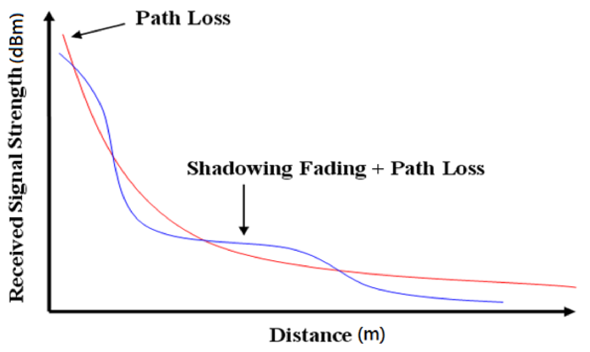
It is mainly used to describe the change of the signal over a long distance (or time), and this change is described in a statistical way to estimate the coverage area of radio waves. Regarding the shadowing effect generated by the terrain and the mobile station, the general literature regards the shadowing effect as a random variable. The shadowing effect will make the received signal power a log-normal distribution as shown in Figure 1.

In the general propagation path loss model, the received power loss caused by the path is influenced by distance. The mobile station will also be affected by neighbors during the movement. Buildings and terrain produce different levels of power loss as expressed by [16,22]:

$$PL\left(dB\right)=PL\left(d_0\right)+10n·\log \frac{d}{d_0}+x_{\sigma }$$

(3)

where $x_{\mathsf{\sigma }}$ (dB) is a log-normal random variable with zero mean and the standard deviation σ = 3–8 dB.

The phenomenon of small-scale fading is used to describe the rapid changes of radio signals after a short period of time/distance. These three phenomena exist at the same time in real channels and are rarely used at the same time due to the high complexity of using them at the same time. Generally speaking, if the research goal is the analysis of system capacity, radio wave coverage area, or handover algorithm, most of the time only the propagation path loss model and the large-scale propagation model will be used. The manual algorithm is related to the long-term and large-scale average signal condition of the system; if the research goal is the processing of the receiver’s fundamental frequency signal, the small-scale propagation model is used for the fundamental frequency signal processing.

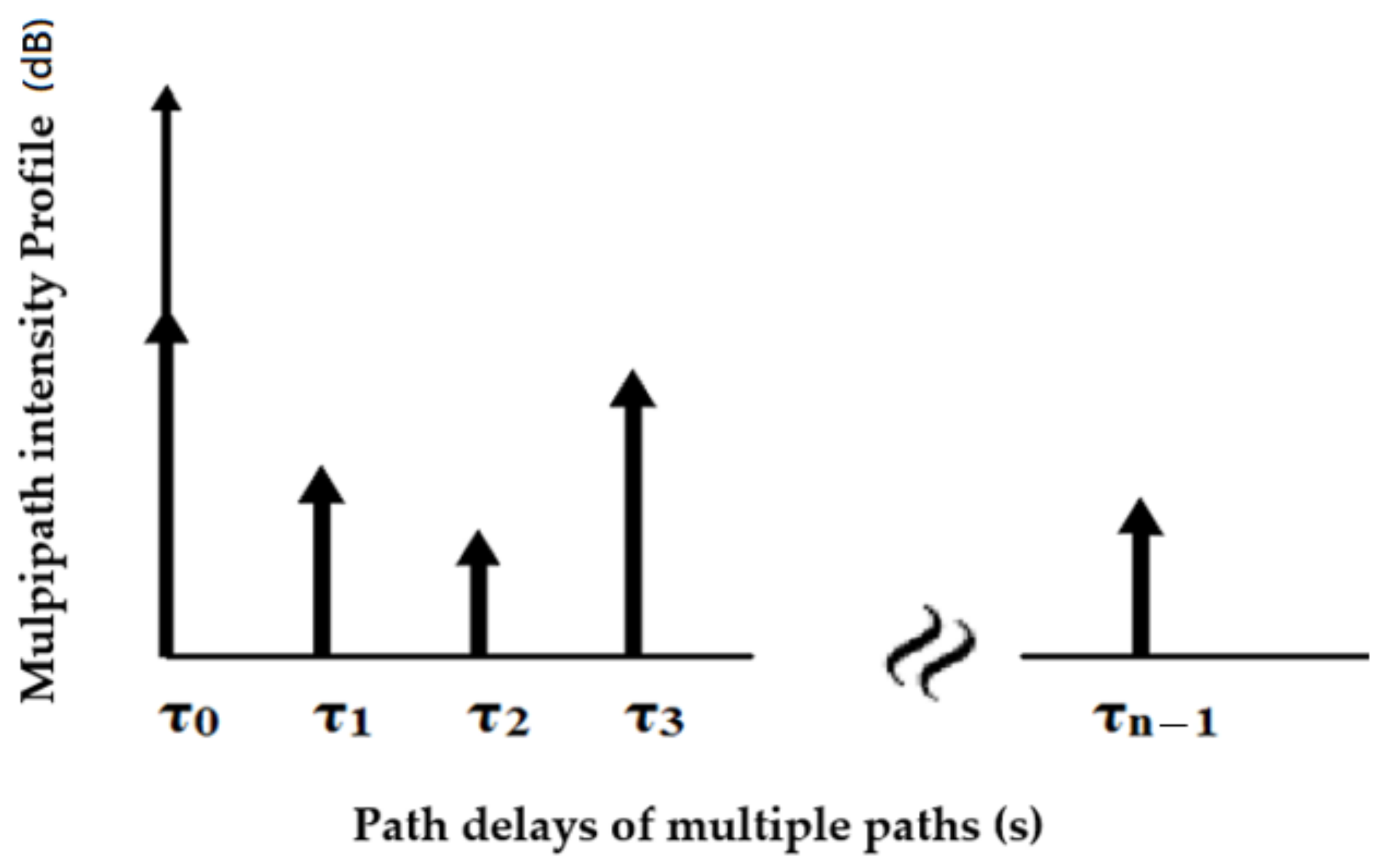
When the signal is transmitted from the transmitter through the wireless channel, it then arrives at the receiving point. It encounters various barriers causing electromagnetic waves to produce reflection, refraction, scattering, and diffraction. When the signal reaches the receiving point, the original signal will become multiple incident signals with different paths. Since each incident signal arrives at a different time, intensity, angle, etc., it causes signal interference and confusion at the receiving point, as shown in Figure 2. The τ₀, τ₁, …, τ_n−1 in Figure 2 are the delays caused by various propagation paths to the receiving point, which are caused by different paths arriving at the receiving point at different times.

The received signal strength method demonstrates that, after the receiving signal point receives the signal strength of the transmitting signal point, it is substituted into the attenuation model to find the distance. In the free-space propagation model, the signal strength received at the receiving point is inversely proportional to the distance. The Foles free-space model calculates the distance between the transmitter and the receiver.

In addition, a model is used to add a masking decay mechanism and a logarithmic normal distribution (σ = 3–8 dB). After the transmitter transmits the signal, there will be obstacles in the propagation path. The greater the difference, the more barriers there are. When the distance between the transmitter and the receiver is d, the average power of the received signal is expressed as shown below [22,23]:

$$P_r\left(d\right)=\frac{P_t{G}_t{G}_r{\lambda }^2}{\left(4{\pi }^2\right)d^{\beta }L}$$

(4)

where $G_t$= 1 is the antenna gain of the transmitting point, $G_r=1$ is the antenna gain of the receiving point, β = 2 is the path attenuation index, and L is log-normal shadowing fading [24].

In the range-based positioning method, RSS is used to estimate the distance between the unknown location and the reference point, the coordinated the value of the unknown node located by the MMSE algorithm.

The positioning performance of MSE and Monte Carlo is used to simulate the average error under different masking and decay environments to obtain the error of different environments. When the three reference nodes used in this paper estimate a known distance, the distance will be obtained separately, and then the known coordinates of the three reference nodes and the three estimated distances are substituted into the MMSE to estimate the position of the unknown node [25,26] as expressed by

$$e_n\left(x_0,y_0\right)={\widehat{d}}_n-\sqrt{{\left(x_n-x_0\right)}^2+{(y_n-y_0)}^2}$$

(5)

where $x_0$ and $y_0$ are the coordinate of the node to be estimated, $x_n$ and $y_n$ are the coordinate of the known reference node, ${\widehat{d}}_n$ is the distance between the n-th reference node coordinate and the node to be estimated, n = 1, 2, 3,..., N.

Triangulation uses the hyperbolic method to calculate the intersection of three circles. The reference node is set to the known reference node coordinates, A, B and C, and the unknown node coordinates are $(x,y)$, assuming that $d_A$, $d_B$, and $d_C$ are the distance from the known node to the unknown node as expressed by [27]:

$$\sqrt{{\left(x-x_A\right)}^2+{(y-y_A)}^2}=d_A$$

(6)

$$\sqrt{{\left(x-x_B\right)}^2+{(y-y_B)}^2}=d_B$$

(7)

$$\sqrt{{\left(x-x_C\right)}^2+{(y-y_C)}^2}=d_C$$

(8)

By Equations (6)–(8), the positioning unknown nodes can be derived by

$$\left[ \begin{array}{c}x\\ y\end{array} \right]={\left[ \begin{array}{c}2\left(x_A-x_C\right)\\ 2\left(x_B-x_C\right)\end{array} \begin{array}{c}2\left(y_A-y_C\right)\\ 2\left(y_B-y_C\right)\end{array}\right]}^{-1} \left[ \begin{array}{c}{x}_A^2-\\ x_B^2-\end{array} \begin{array}{c}{x}_C^2-\\ x_C^2-\end{array}\begin{array}{c}{y}_A^2-\\ y_B^2-\end{array}\begin{array}{c}{y}_C^2-\\ y_C^2-\end{array}\begin{array}{c}{d}_C^2-\\ d_C^2-\end{array}\begin{array}{c}{d}_A^2\\ d_B^2\end{array}\right]$$

(9)

Because this positioning method can provide better accurate positioning when there is no error in the three distances. When the distance is in error, it is impossible to determine a clear coordinate point and the MMSE is proposed for solving this problem.

3. External Distance Variation Methods

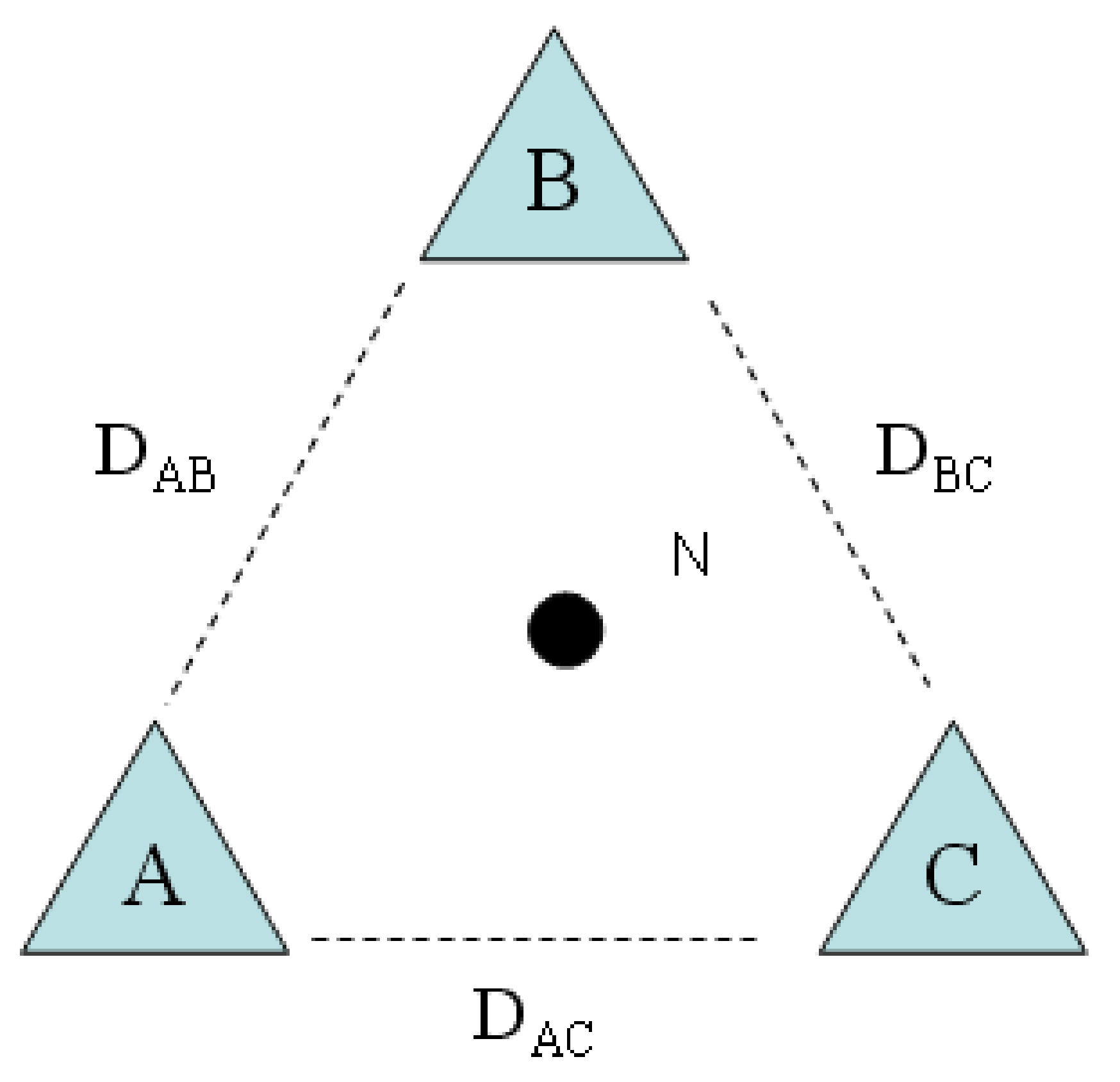
In the selection mechanism, Figure 3 shows that nodes A, B, and C are reference nodes and that the dashed line is the external distance variation. In order to calculate positioning, four or more reference nodes are selected with closest to the positioning node and three reference nodes are finally selected.

After selecting three suitable reference nodes, to calculate the average distance, $D_{Outer}$ for any three reference nodes is shown by

$$D_{Outer}=\frac{D_{AB}+D_{BC}+D_{AC}}{3}$$

(10)

where the $D_{AB}, D_{BC}$, and $D_{AC}$ are the distances from the three reference nodes of A, B, and C to the positioning node, respectively. These three reference nodes with the smallest ${\sigma }_{Outer}^2$ are selected as the positioning estimation [23]. Then, the variation of the outer distance ${\sigma }_{Outer}^2$ is calculated by

$${\sigma }_{Outer}^2=\frac{{(D_{AB}-D_{Outer})}^2+{(D_{BC}-D_{Outer})}^2+{(D_{AC}-D_{Outer})}^2}{3}$$

(11)

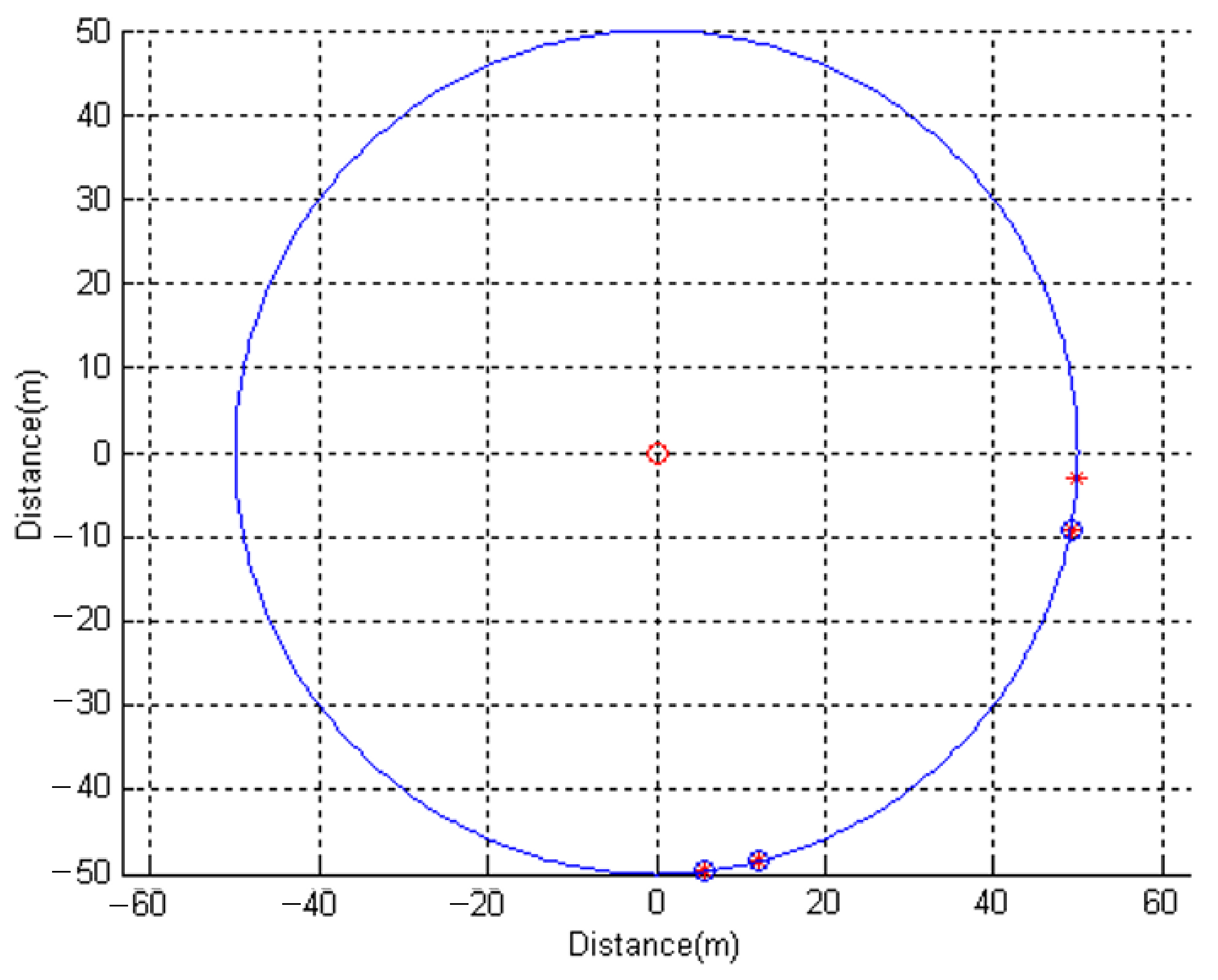
Since the external variation is selected, unsuitable nodes may be selected to increase the probability of MSE. Figure 4 is considered for the external variation that the distances from the reference nodes deployed on the circle to the center of the circle are all the same. This model is used to explore the influence of the MSE caused by the distribution of the deployment. Figure 4 shows that four reference nodes are randomly deployed on the circle, and the smallest amount of variation and the corresponding three reference nodes will be selected through the four-to-three mechanism. The circled circle is the selected reference node. These three reference nodes are the smallest by calculating the variation and the MSE is very high here [23].

In Figure 5, there are two reference nodes that are very close to each other, and the MSE is also very high. Therefore, how to deploy the reference node to reduce the MSE is one of the key points in this paper. The MSE of the reference node deployed in Figure 6 is greatly reduced after the selection mechanism.

As seen from Figure 4, Figure 5 and Figure 6, when two of the reference nodes are very close, the value of MSE is higher. A judgment type is added to strengthen the function of the selection mechanism and to avoid selecting unsuitable deployments. Therefore, this paper proposes two conditions: first, the distance of $\overline{AB}$, $\overline{BC}$, and $\overline{AC}$ is less than the threshold value $D_m$; and second, the average distance of the three segments is less than the threshold value $D_{av}$. If the selected three points of A, B, and C meet any one of the conditions, the reference points of A, B, and C are selected and eliminated.

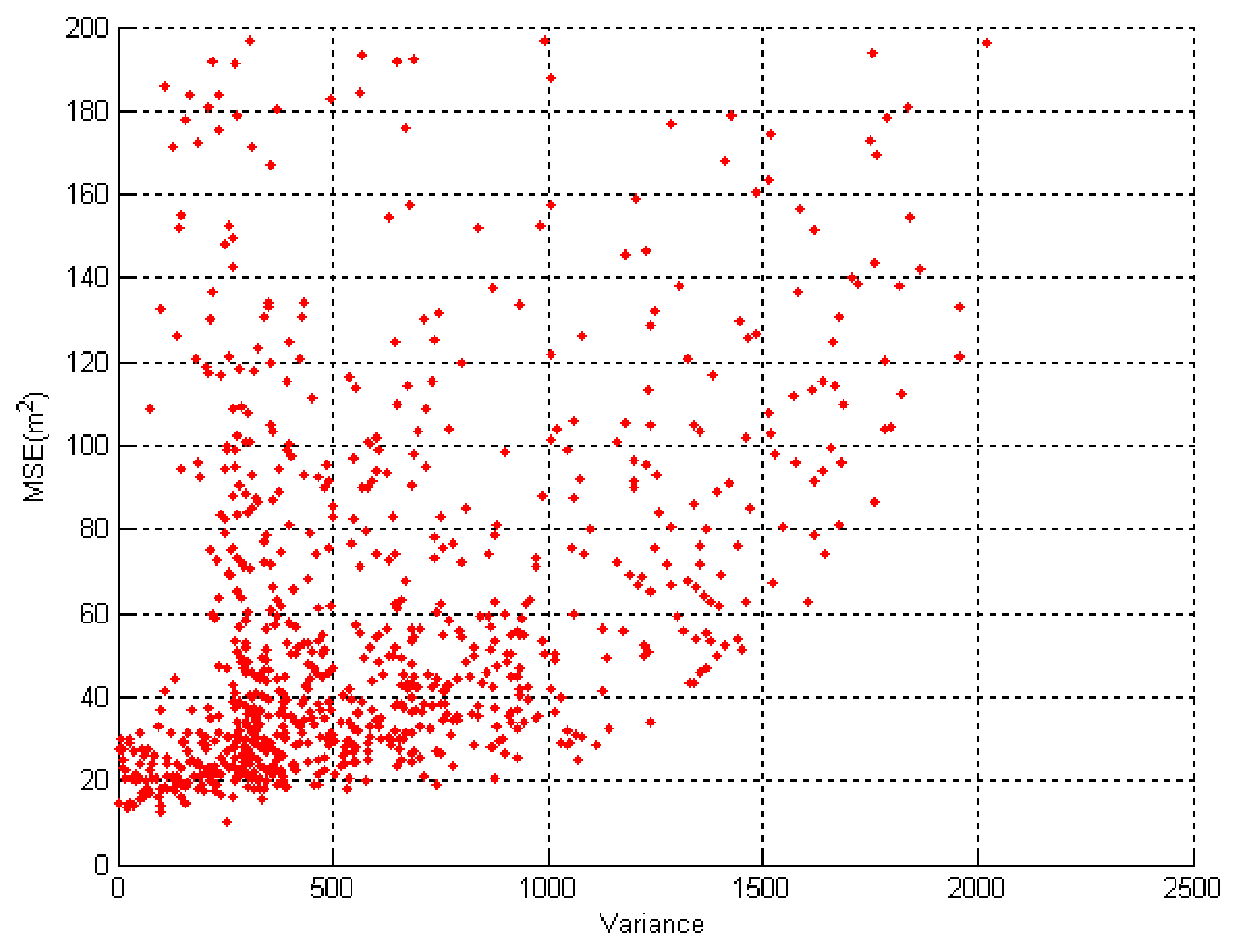
Figure 7 indicates that the selected three reference nodes are very close to each other and that the distance variation is small with higher MSE. Therefore, a conditional expression should be added to reduce the probability of this.

Figure 8 supposes that the conditions are $D_m$ ≤ 20 and $D_{av}$ ≤ 70. When the distance variation is greater, the probability of relative MSE is increased. When the four reference nodes are selected through the selection mechanism, the variation of the distance between the selected three reference nodes is the smallest. The variance value of the distance can determine the deployment status of the three reference nodes. Therefore, the greater the distance variation, the greater the probability that the three reference nodes of the deployment will approach, and so the probability of MSE will increase and be greater. This paper adds two more conditions that are $D_m$ ≤ 10 and $D_{av}$ ≤ 60. 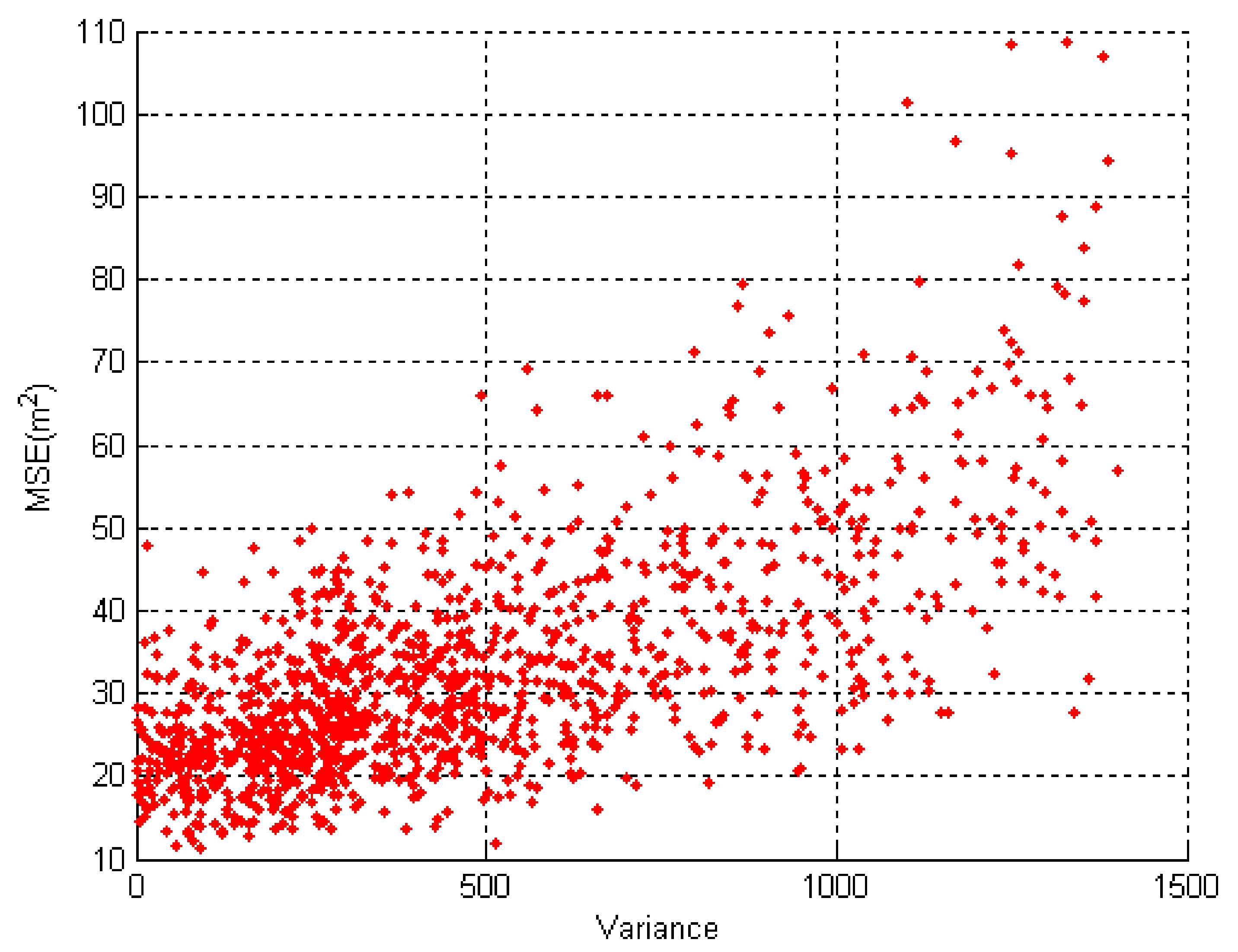Figure 8 compares the external distance variation of three out of four choices. When 10 to 30 reference nodes are deployed, it is obvious that the value of MSE is dropped.

Table 2. Comparison of conditions added and choosing three from four mechanisms.

Number of Deployment Reference Nodes	Three From Four Mechanism	Strengthen the Selection Mechanism
10 reference nodes	77.086	67.61
20 reference nodes	60.31	56.87
30 reference nodes	50.32	49.12

compares the external distance variation between the selection mechanism and the selection mechanism of four out of three options, showing that MSE is still improved when the addition conditions are at different reference nodes.

4. Results

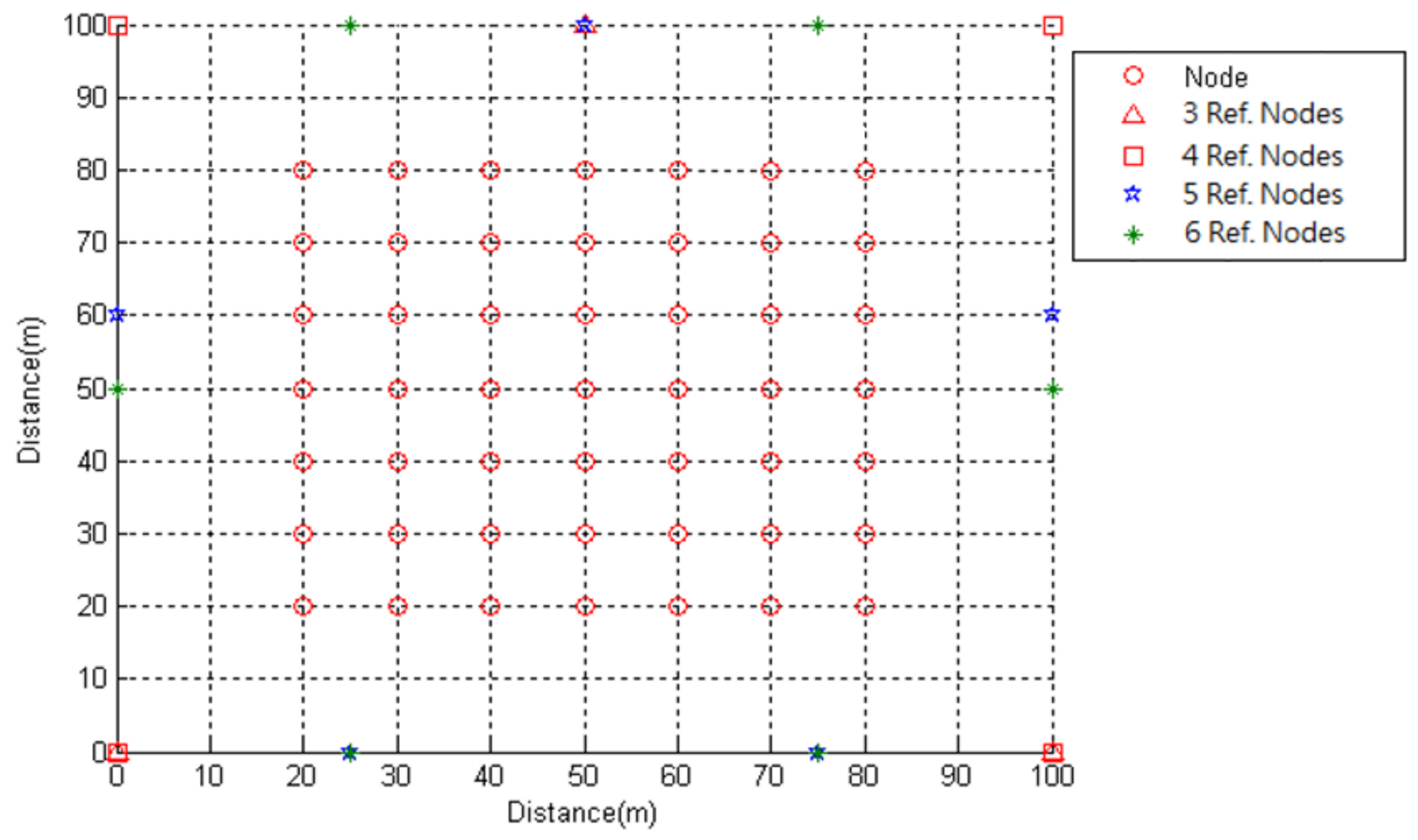
Simulation environment in this paper is about a 100 m × 100 m using the MMSE algorithm to locate the area formed by the circle as shown in Figure 9 and Figure 10. Figure 9 and Figure 10 are either defined as a small area and a large area, respectively, for comparison for two MSEs. Furthermore, in Figure 9 and Figure 10, three to six fixed reference nodes are used to estimate the small range and the large range, respectively. When more reference nodes are used to estimate for results, the MSE is decreased. 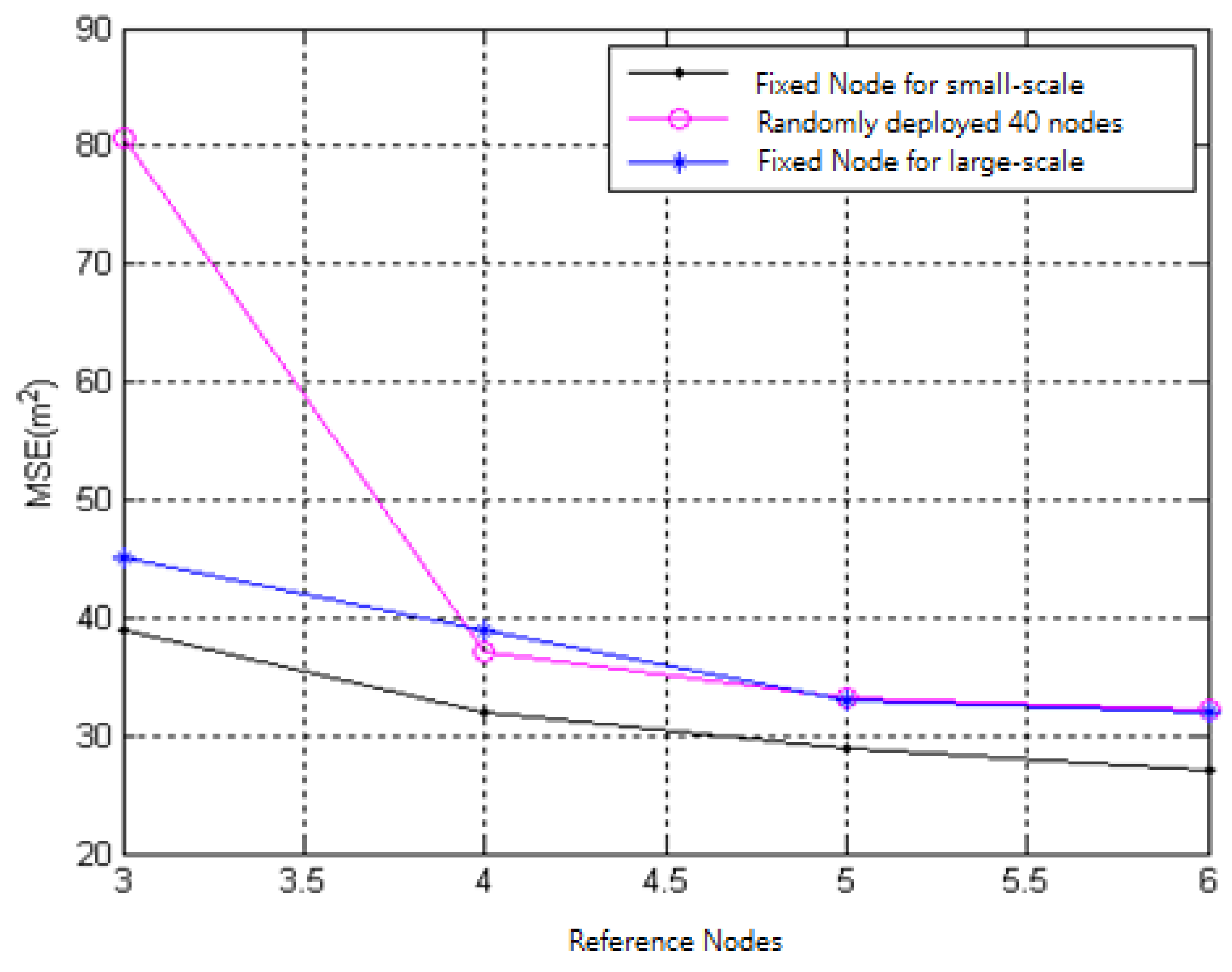Figure 11 compares the MSE of three to six fixed and randomly deployed 40 reference nodes. The more reference nodes there are, the more MSE decreases, and the lower the MSE of the fixed reference node.

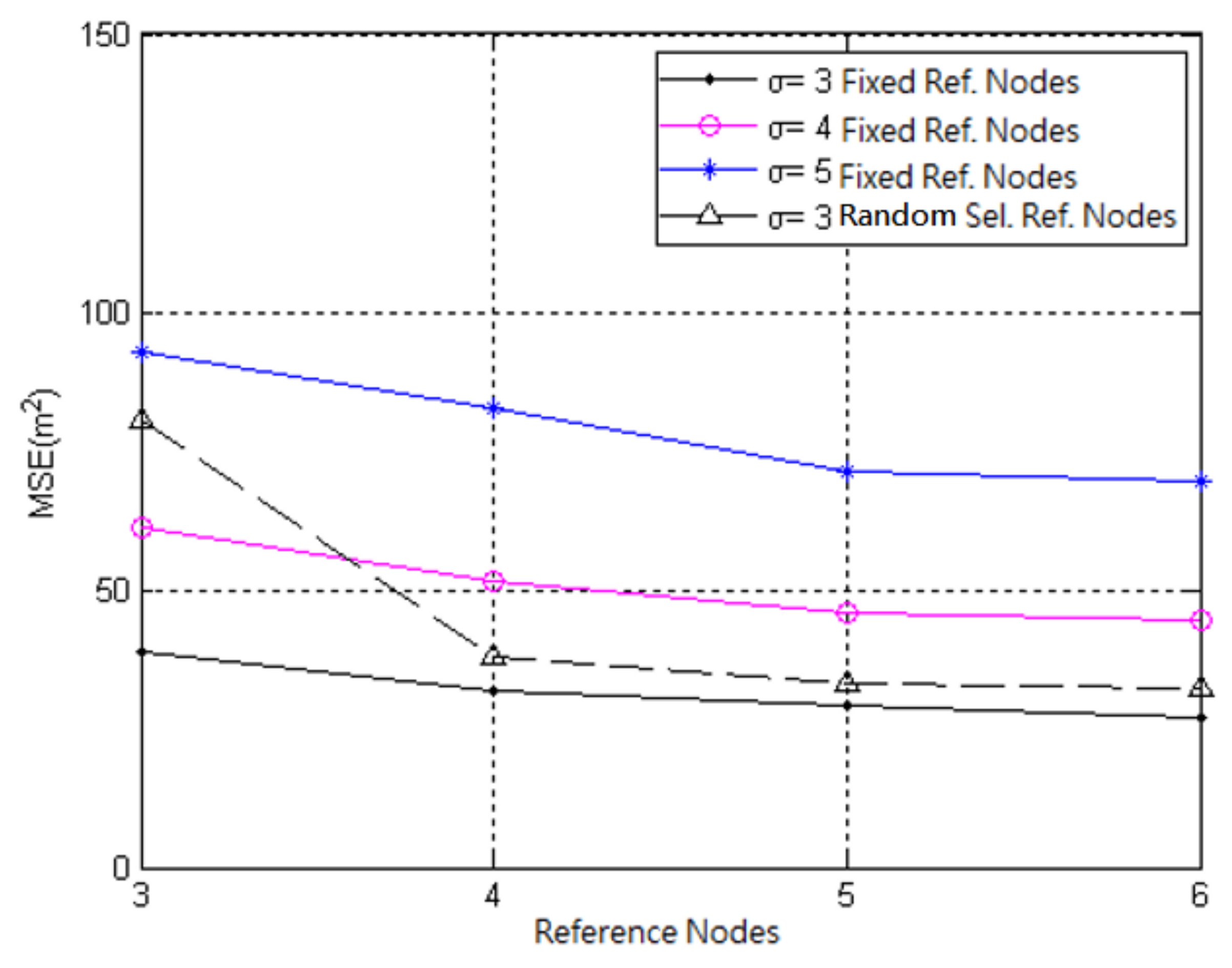
In Figure 12, the random selection of reference nodes (σ = 3) is added to a small range. The random selection of three reference nodes (σ = 3) is higher than the fixed three (σ = 4) MSEs. Because three random reference nodes may be selected as reference nodes that are very close to each other and will increase the MSE. When there are four at random, the MSE will be a little bit higher than the fixed three (σ = 3) because the original three reference nodes are very close and the MSE will be very high. If one more reference node supports positioning, the MSE will be lower than the original three reference nodes.

In Figure 13, the method of randomly selecting reference nodes (σ = 3) is added in a large range. Although the fixed three (σ = 4) and the random three (σ = 3) are compared with the random three (σ = 3), the random three (σ = 3) are worse. The reference nodes 4, 5, and 6 are both fixed and random.

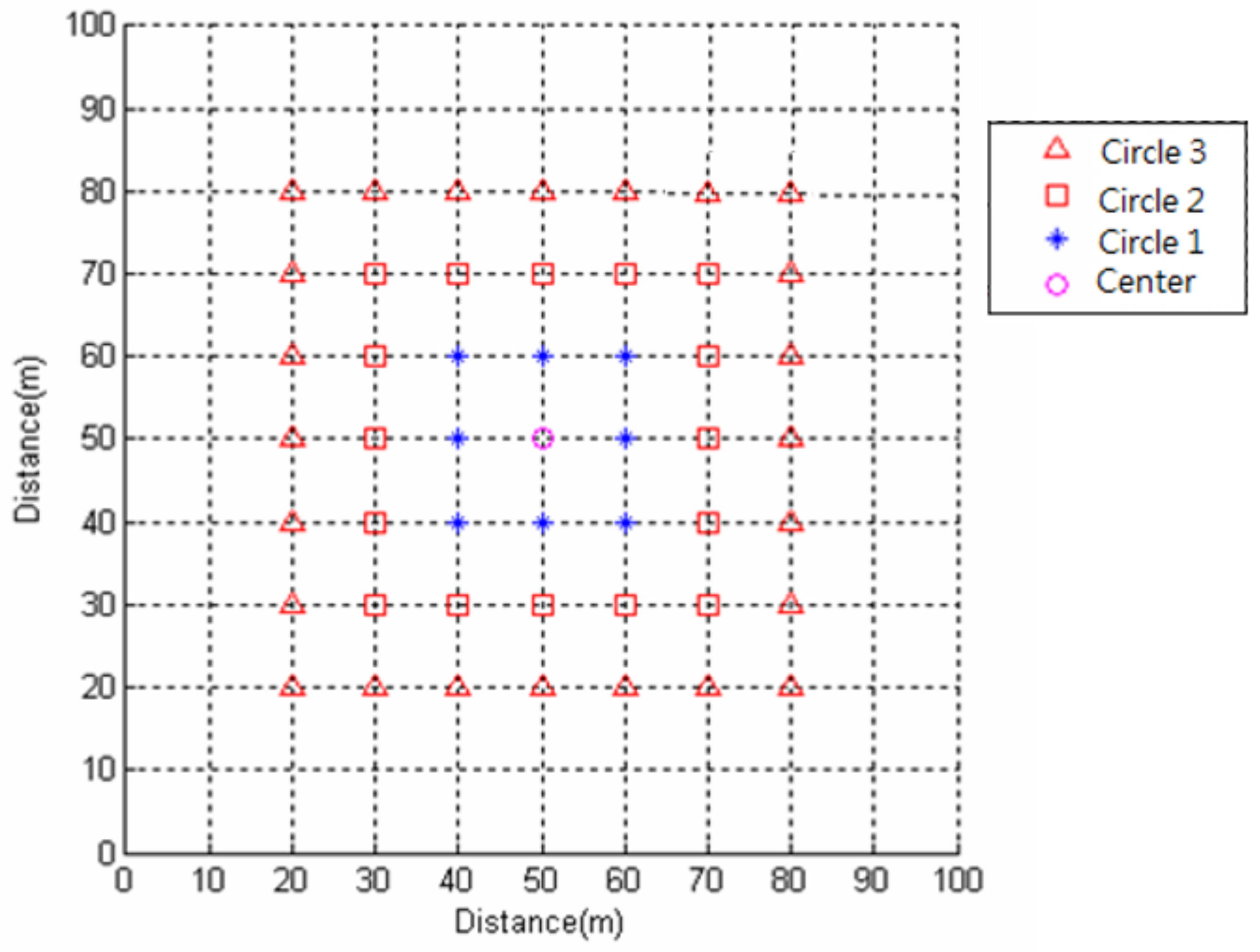
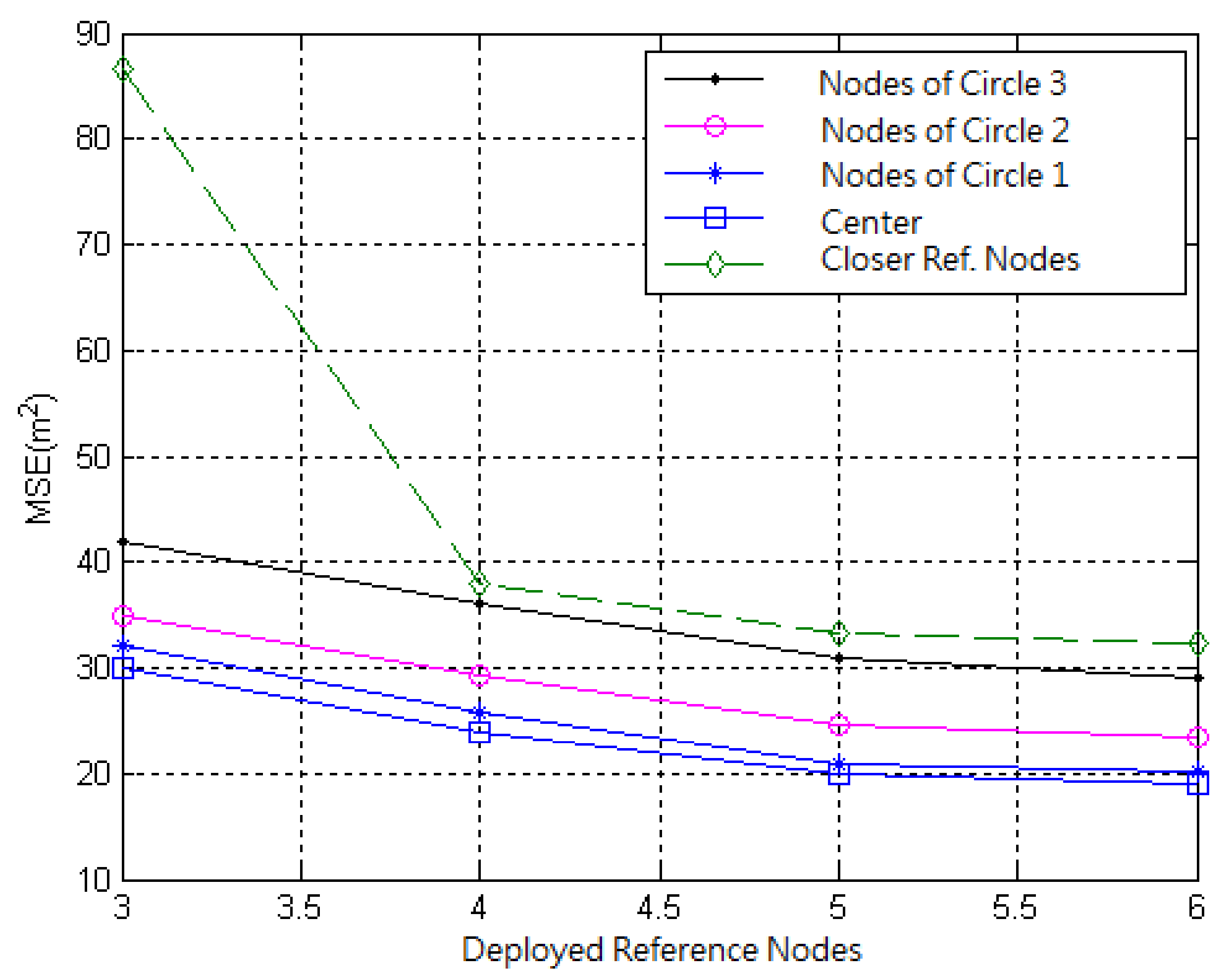
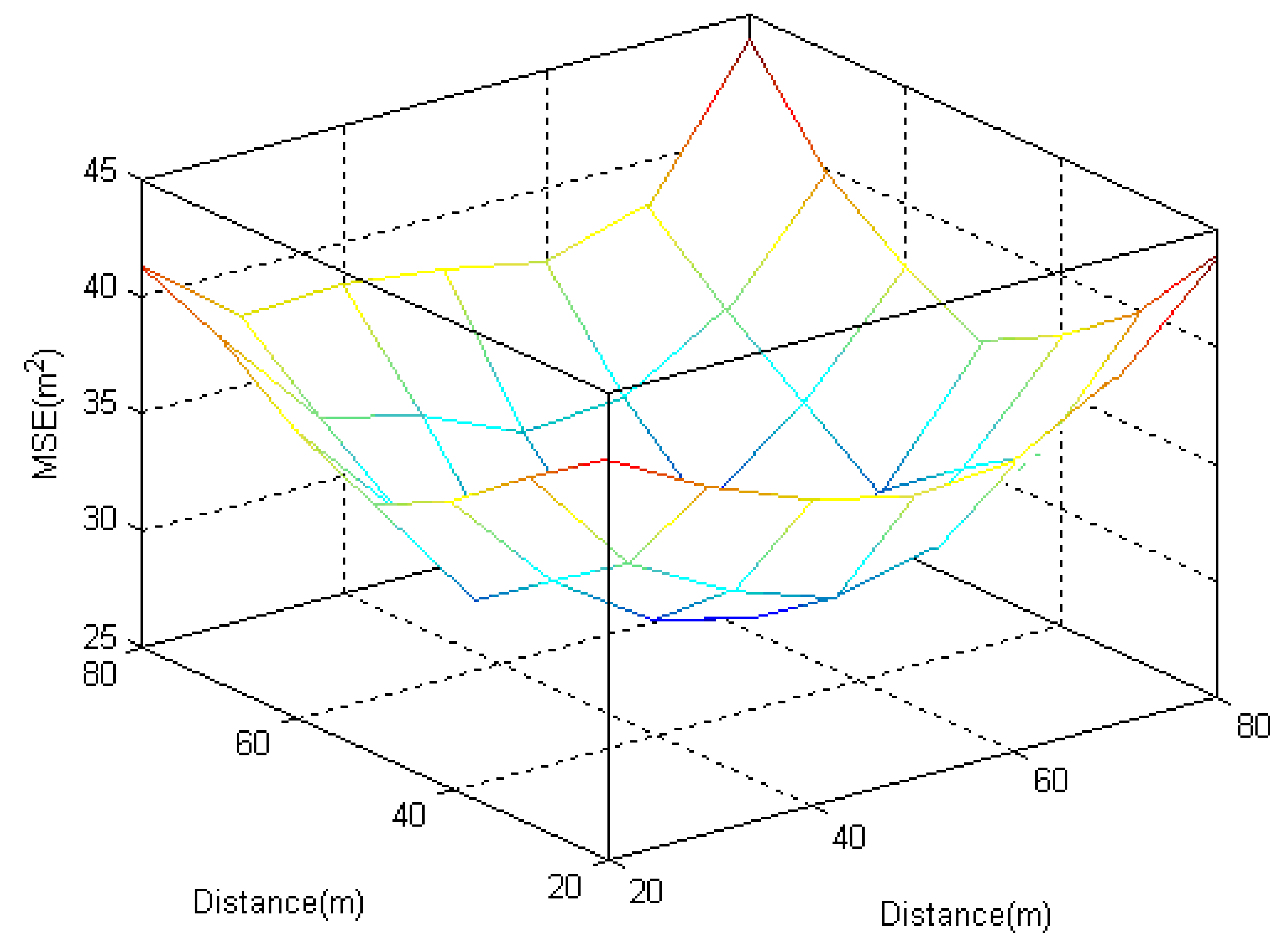
The analysis method is based on the center coordinates (50, 50). As shown in Figure 14, the square extended outward is defined as the first circle to the third circle. The change of MSE around the center point can be explored. As shown in Figure 15, the MSE of the center point coordinates (50, 50) is the lowest, and the MSE will increase. Therefore, the MSE of the outermost periphery (the first circle) is the highest, whereas the fixed reference node is higher than the MSE of the random deployment reference node.

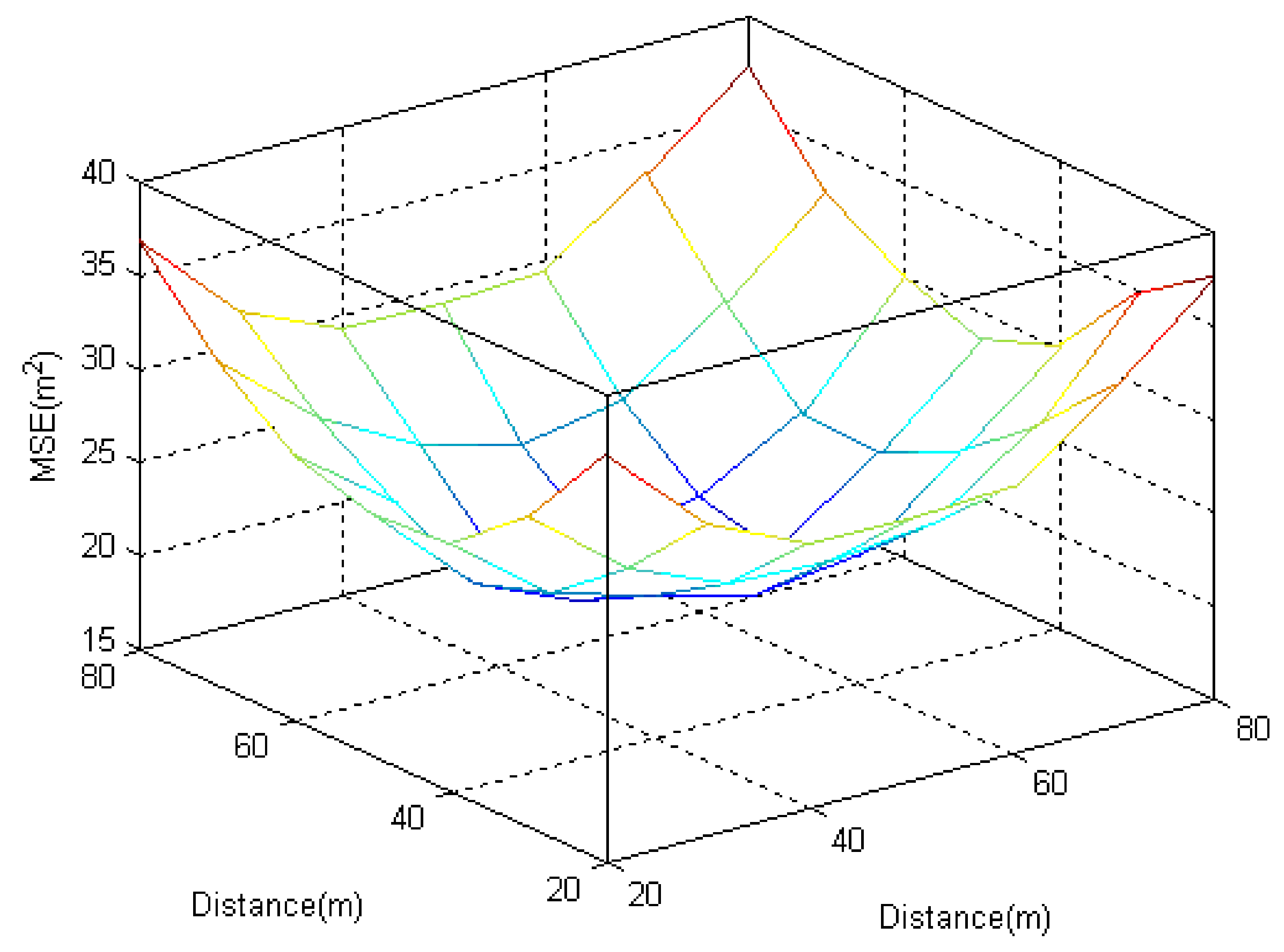
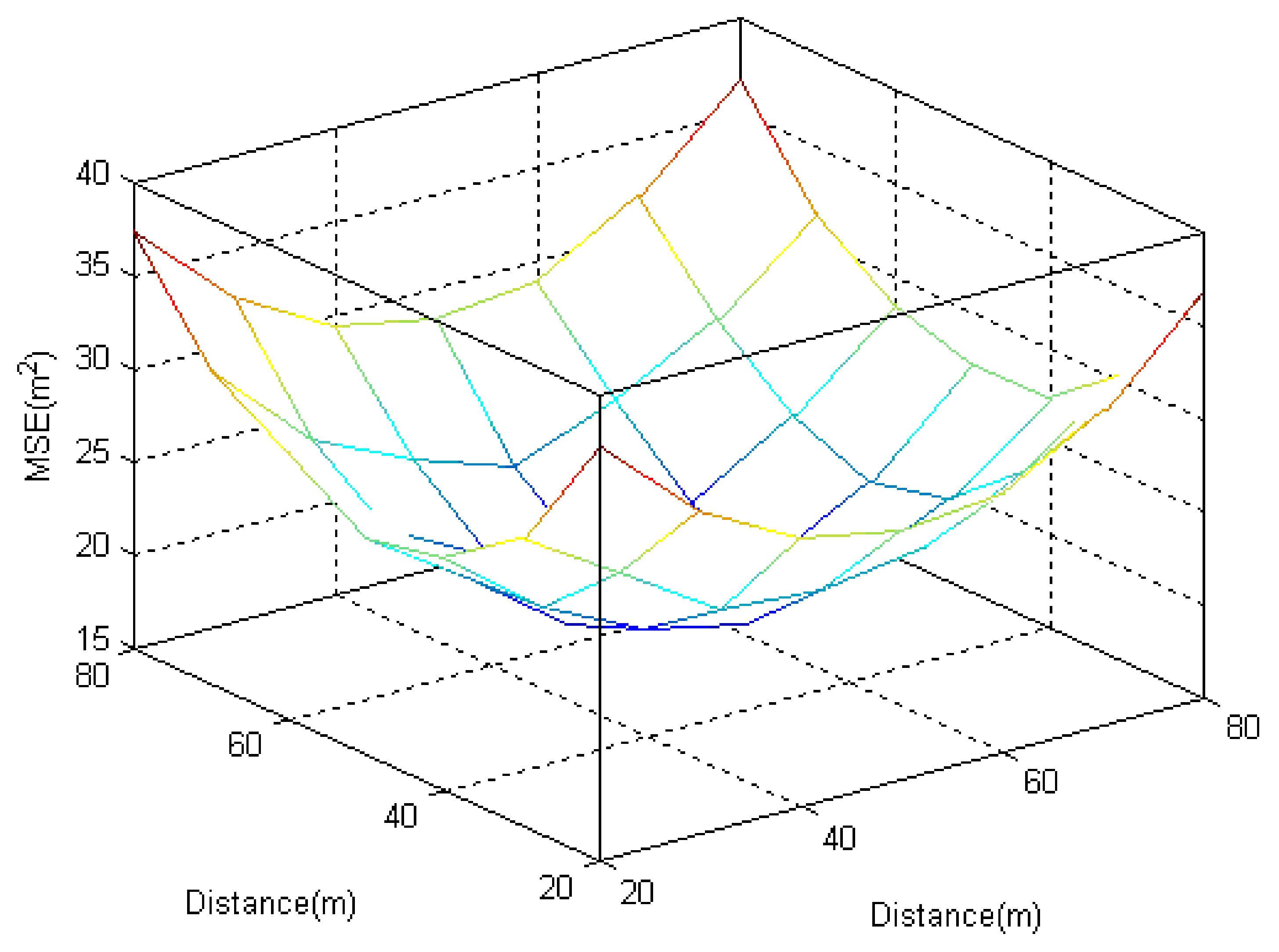
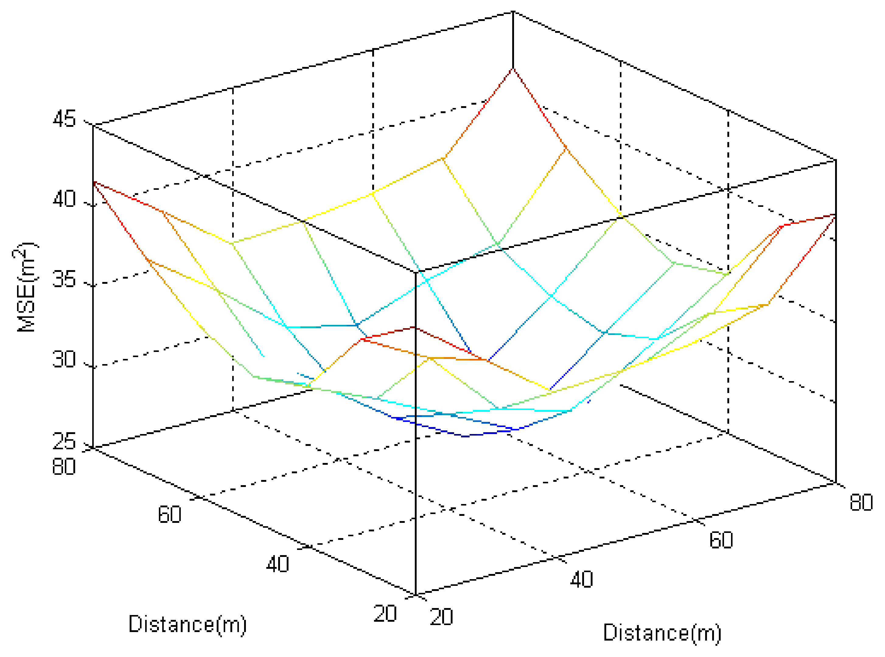
However, by analyzing the fixed three, four, five, and six reference nodes through the 3D graph to estimate the small area, the difference between them can be more clearly observed. As shown in Figure 16, when the three reference nodes are fixed to estimate the nodes, the closer they are to the center point, the lower the MSE, and the highest relative to the outermost node. Therefore, from Figure 16, Figure 17, Figure 18 and Figure 19, it is shown that the lowest MSE is the center point coordinates (50, 50), and that the highest MSE is around a small area. The more reference nodes are located, the MSE of the node will decrease.

5. Conclusions

The internal and external variation mechanism are matched to analyze the influence of MSE caused by positioning. This paper proposes the signal strength to estimate the distance and the MMSE algorithm to explore the effectiveness of indoor positioning. Experiments show that the positioning MSE and positioning node are referenced. The amount of variation in the distance between nodes is related. In order to improve the positioning accuracy, this paper proposes to use the internal distance (the distance between the positioning node and the reference node) and the external distance (the distance between the reference nodes) to select the most suitable reference node. However, unsuitable nodes may be selected to increase the probability of MSE. Therefore, this paper considers the model of external variation. Because the distance from the reference node to the center of the circle is the same, this model is also used to discuss the layout. Four reference nodes are randomly deployed on the circle, and the smallest amount of variation and the corresponding three reference nodes will be selected through the four-select-three mechanism. After calculating the three reference nodes, the amount of variation is minimal and the MSE is very high. Finally, this paper analyzes several reference nodes (three, four, five, and six reference nodes) through 3D graphs to estimate the small range area. The differences are more clearly observed with fewer reference nodes and with lower MSE. Simulation results show that the MSE value of fixed three reference nodes is almost 100% better with the external distance variation method compared to the random selected three reference nodes.