
Optimal Base Station Location for Network Lifetime Maximization in Wireless Sensor Network


Abstract
:1. Introduction
- To optimize the location of the base station, an efficient energy-saving technique called the crossover elitist conservation genetic algorithm (CECGA) was suggested, where in the crossover phase, we apply the elitist conservation of individuals to replace others in the second generation. To avoid the loss of the best chromosome after mutation, elitism is used to copy some of those chromosomes for the next generation. This optimal location helps reduce the distance from nodes to the base station, which results in saving energy used by nodes.
- Data transmission from nodes to the base station consume a high amount of energy that can cause the network to stop working early; to solve this problem, the K-medoids algorithm for nodes clustering is proposed for choosing the appropriate cluster head to acquire the perfect outcome of the cluster, to prevent the adverse effect of outliers, and to calculate the optimum medoids among the sensor nodes.
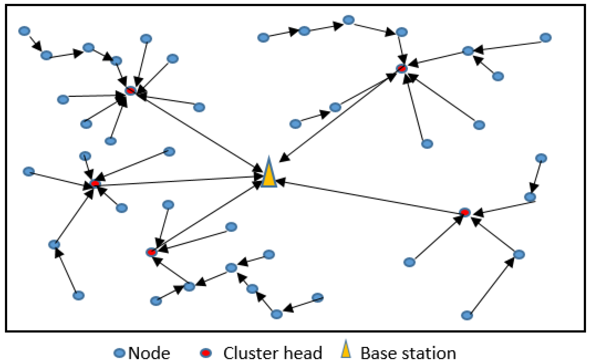
- After forming clusters, a multi-hop data routing is used among sensor nodes inside the cluster to send sensed data to their cluster heads from node to the nearest node, which results in reducing energy use in the cluster.
2. Literature Review
3. Network Model
3.1. The Proposed Network Model
3.2. Energy Model
4. Proposed Approaches
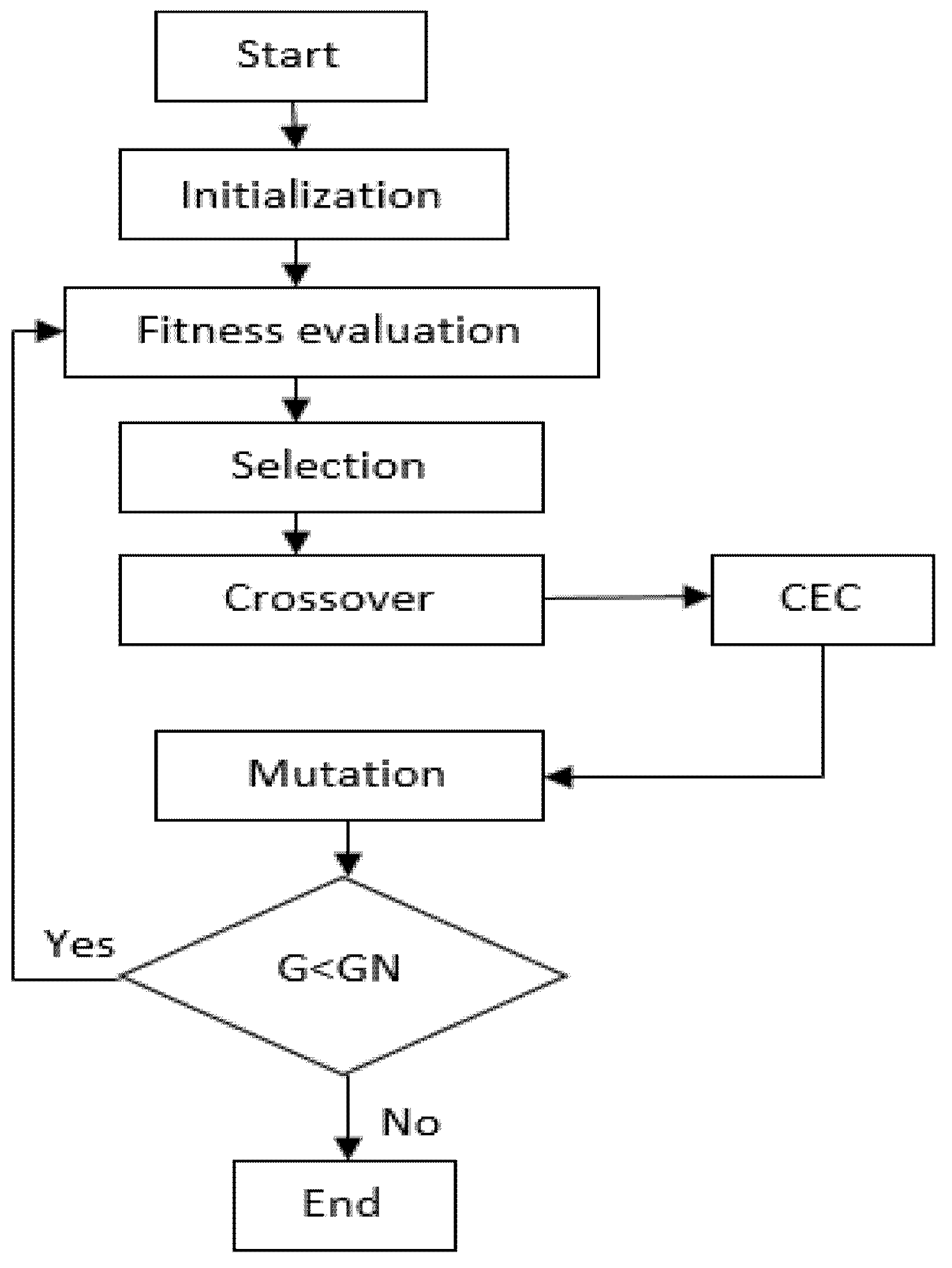
4.1. Crossover Elitist Conservation Genetic Algorithm (CECGA)
- Population Initialization: Firstly, random 𝑁 individuals (chromosomes) are produced, and the evolutionary generation begins with iteration 0. The distance threshold (communication radius) is initialized.
- Fitness Calculation: To evaluate if the particular chromosome increases or decreases the lifetime of WSN, we calculate its fitness function. The algorithm conserves the historically obtained best chromosome; that is, with the highest fitness value, this is called elitism. The fitness of a chromosome controls how much energy is consumed and how much coverage is provided. Our algorithm fitness is a cluster-based distance (CD), which is the sum of the distances between the calculated member nodes and their cluster leaders, as well as the total CHs and BS distances, and is calculated as follows:where n and m denote the number of clusters and related members, respectively; dij is the distance between a node and its CH; and DCB denotes the distance between the CH and the BS. The solution is best suited for networks with a high number of widely separated nodes. A greater cluster distance results in higher energy usage. This measurement is used to manage the density of the clusters, where density is the number of nodes in each cluster.
- 3.
- Selection: The selection step chose the best individuals according to the selection operator, whereby a mating pool of individuals with above-average fitness values is conserved and two parents become selected randomly for crossover.
- 4.
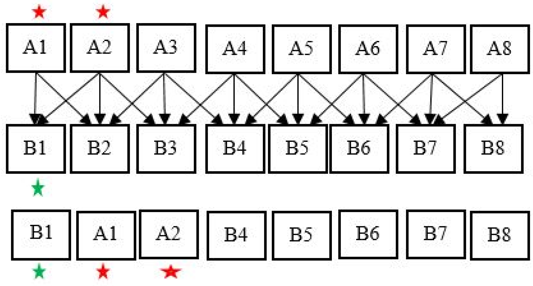
- Crossover: CECGA is used to obtain better parameters. In the crossover phase, we apply the elitist conservation of individuals to replace others in the second generation. To avoid the loss of the best chromosome after mutation, elitism is used to copy some of those chromosomes in the next generation.
- 5.
- Mutation: The new individuals are produced in this mutation to keep the diversity in the population. Here the node is selected randomly from the best chromosome obtained in the past generation.
| Algorithm 1 Crossover Elitist Conservation Genetic Algorithm |
| Input: (1) Population size N, (2) Number of generation NG, (3) Elitists e 1. Initial the current population P 2. Calculate the fitness 3. Selection 4. For i = 1 to NG 5. Crossover // Crossover Elitist Conservation Mechanism (CEC) // 6. For j = 1 to N 7. Find the last optimal solution B1 8. If the current solution Bj < B1 9. B1 = B 10. e = A1 (B1’s father) and A2 (B1’s mother) 11. End 12. Next i 13. e ⸦ Next P // End of Crossover Elitist Conservation Mechanism (CEC) 14. Mutation 15. Evaluation of the population P 16. Update B1 17. Next j Output: The optimal solution B1 |
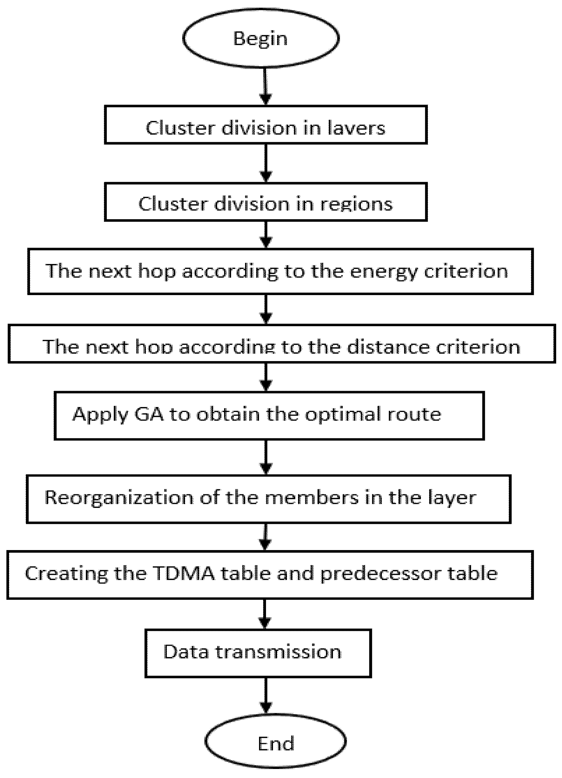
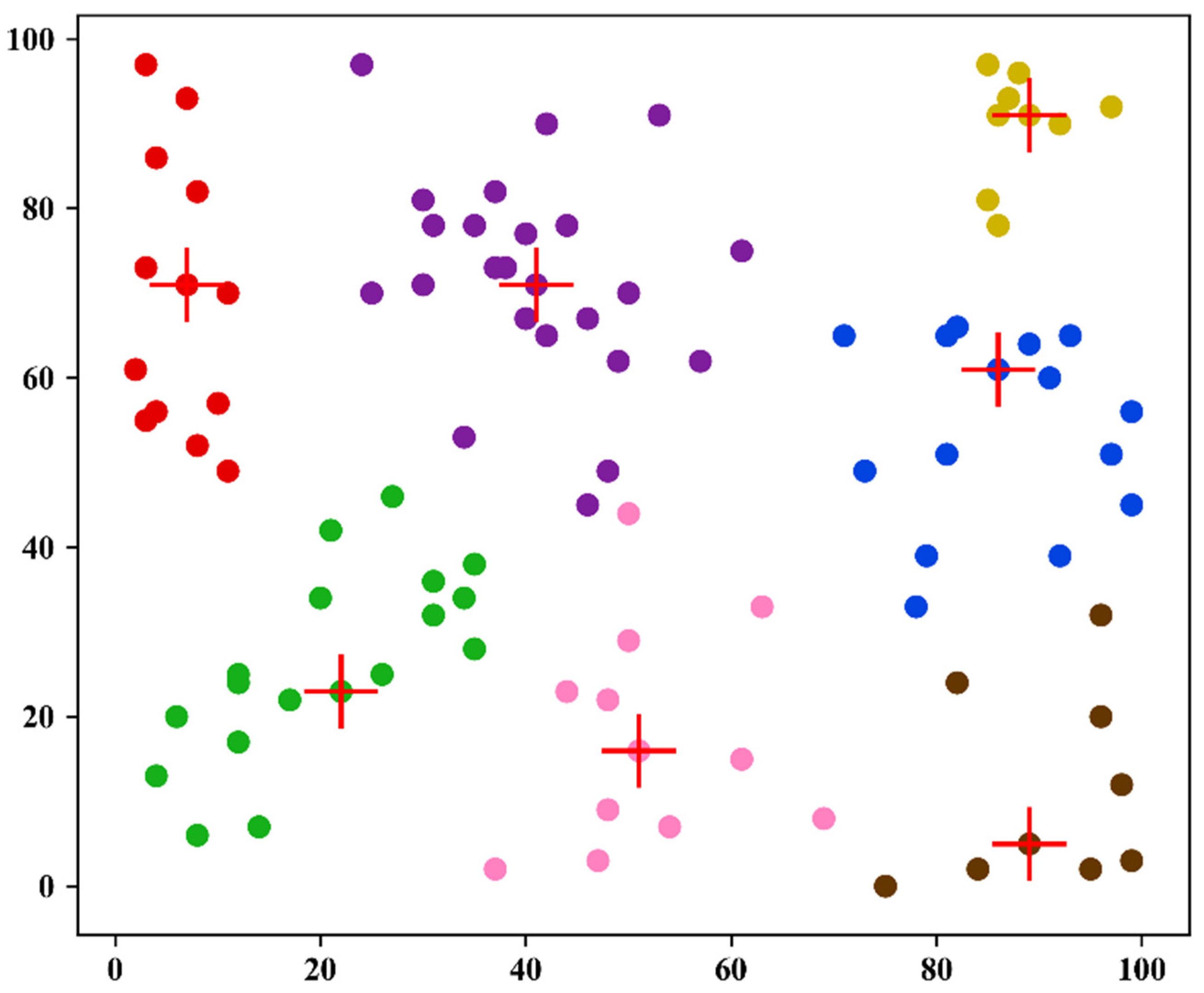
4.2. Proposed Routing Based K-Medoids Clustering
- They fixed the number of layers to 4, whereas in our approach. we set 10 nodes in one layer, which means if we used 100 nodes, then we will obtainwhere L represents the number of layers and N is the number of nodes in the field.
- In their work where 4 layers are used, nodes in layer number 4 must only communicate with nodes in layer number 3 and so on, and finally, nodes in layer 1 connect directly to the base station. Here it does not make sense because nodes in layer 4 can be closer to the node in layer 2, thereby assuming that the number of nodes in each layer is set to 10, a total of 100 nodes, then divided into ten layers. For layer 10 nodes, we traverse all nodes in layers 1–9 and find a connection to the nearest node. For layer 9 nodes, we traverse all the nodes in layers 1–8 to find the closest node to connect sequentially.
- In their approach for nodes in layer 4, for example, there is one common closer node in the next layer, and if all these nodes send data to its closest node, then that node will be down fast because it is using more energy to receive data, so its life is very short. Here the improvement is to impose a penalty when calculating the distance between nodes, and the specific formula is:where d(i, j) denotes the distance between nodes i and j. Ki represents the number of nodes connected to sensor node i. After constructing the routing from nodes to their cluster heads, these cluster heads send data corrected to the optimal base station calculated above.
5. Experimental Results Assessment and Discussions
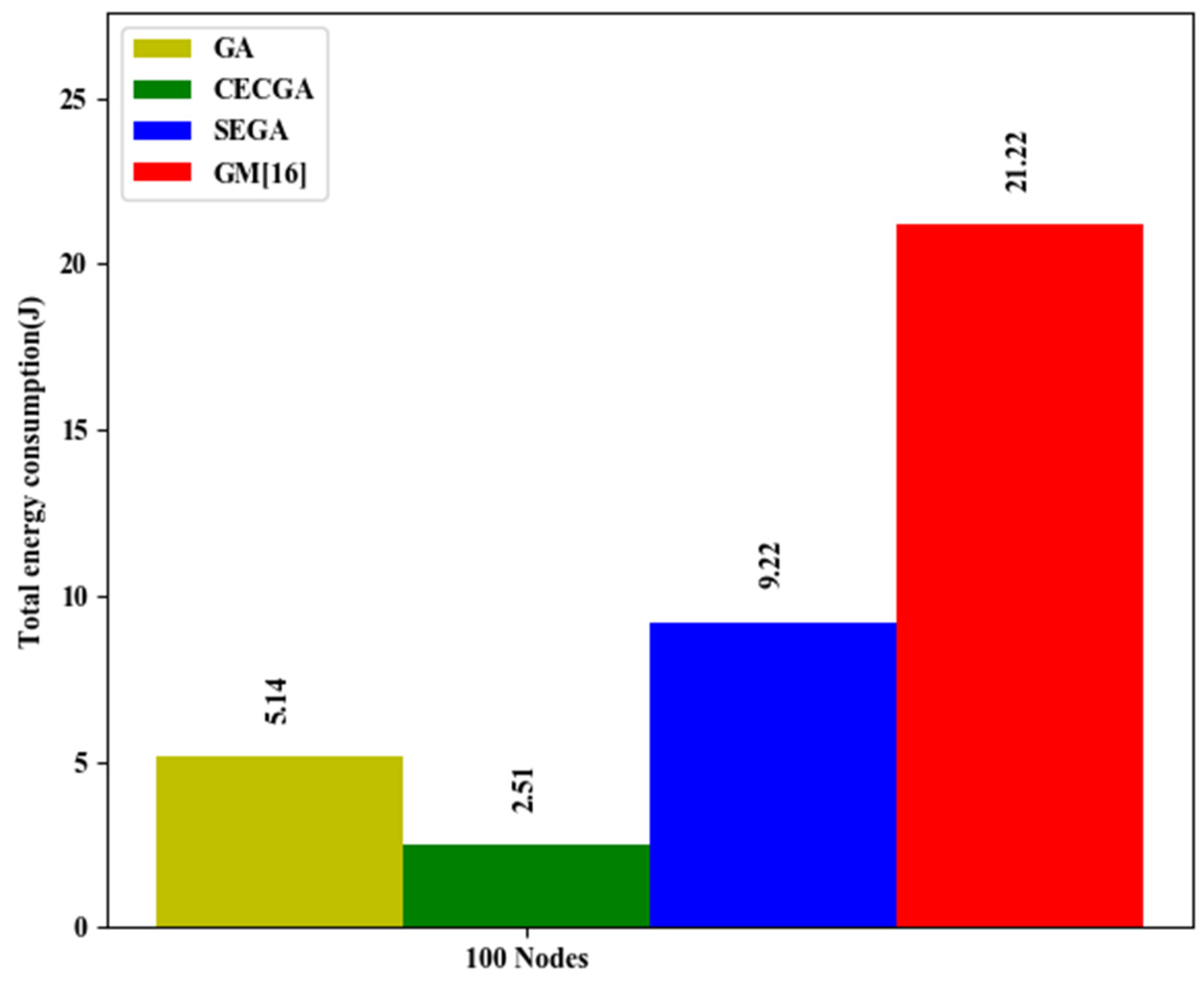
- Energy Consumption—The total energy consumed during a round can provide a good estimate of the algorithm’s energy efficiency, and the total energy consumed increases as the number of generations increases.
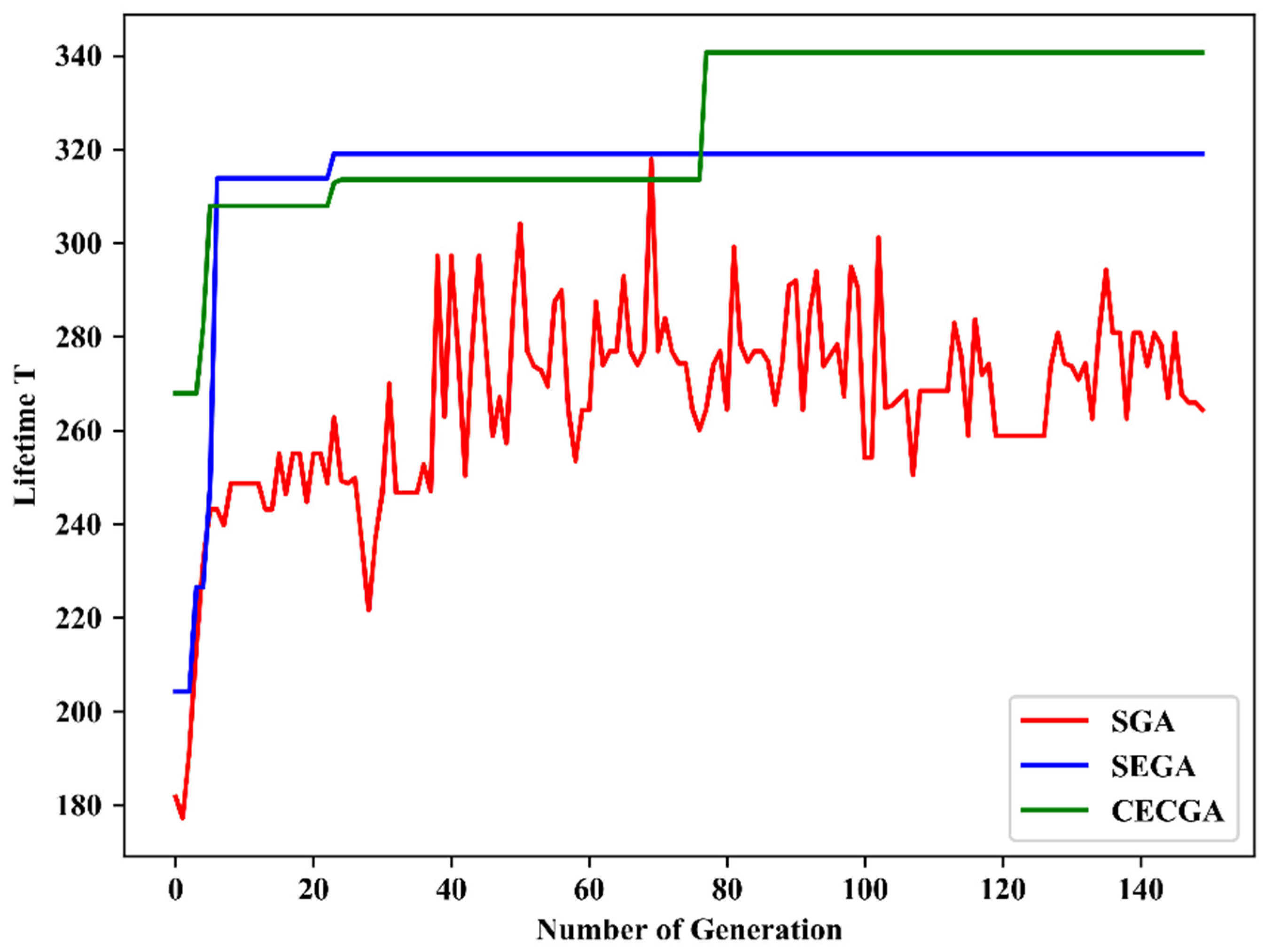
- Network Lifetime—The network lifetime is defined as the time when all sensor nodes stop functioning.
- First Node Death—Our work plots the first node death by showing which round the first node dies by comparing different BS locations in different networks.
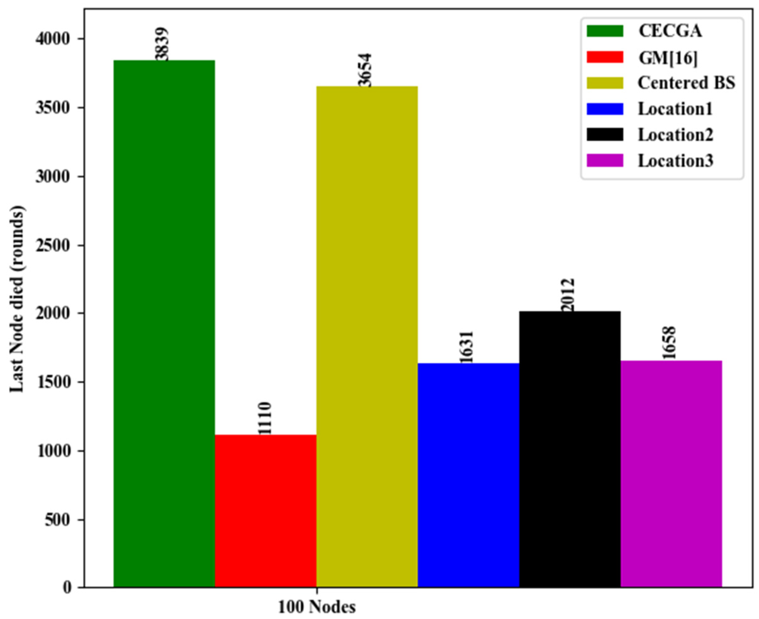
- Last Nodes death—Our work plots the last node death by showing which round the first node dies by comparing different BS locations in different networks.
6. Conclusions and Future Work
Author Contributions
Funding
Institutional Review Board Statement
Informed Consent Statement
Data Availability Statement
Acknowledgments
Conflicts of Interest
Abbreviations
| AoI | Area of interest |
| BS | Base station |
| CECGA | Crossover elitist conservation genetic algorithm |
| CH | Cluster head |
| dij | Distance between sensor i and sensor j (or base station B) |
| SGA | Simple genetic algorithm |
| GM | Geometric median |
| i, j | Nodes |
| KMC | K-medoids clustering |
| LEACH | Low energy adaptive clustering hierarchy |
| N | Number of sensor nodes |
| R | Data rate |
| SEGA | Straighten elitist genetic algorithm |
| SN | Sensor node |
| T | Network lifetime |
| Vij, ViB | Power consumption coefficient for transmitting data from sensor i to sensor j and i to the base station |
| Wij, WiB | Data rate from node i to j and from i to base station |
| WSN | Wireless sensor network |
| XB, YB | Coordinates of base station |
| α | The path-loss index |
| β1 and β2 | Constant coefficients in transmission power modeling |
| ρ | Constant coefficient |
| Pi | Rate of energy consumption at sensor node i |
References
- Lara-Cueva, R.A.; Gordillo, R.; Valencia, L.; Benitez, D.S. Determining the main CSMA parameters for adequate performance of WSN for real-time volcano monitoring system applications. IEEE Sens. J. 2016, 17, 1493–1502. [Google Scholar] [CrossRef]
- Rotariu, C.; Bozomitu, R.G.; Cehan, V.; Pasarica, A.; Costin, H. A wireless sensor network for remote monitoring of bioimpedance. In Proceedings of the 2015 38th International Spring Seminar on Electronics Technology (ISSE), Eger, Hungary, 6–10 May 2015; pp. 487–490. [Google Scholar]
- Mahamuni, C.V. A military surveillance system based on wireless sensor networks with extended coverage life. In Proceedings of the 2016 International Conference on Global Trends in Signal Processing, Information Computing and Communication (ICGTSPICC), Jalgaon, India, 22–24 December 2016; pp. 375–381. [Google Scholar]
- Zhong, S.; Zhong, H.; Huang, X.; Yang, P.; Shi, J.; Xie, L.; Wang, K. Security and Privacy for Next-Generation Wireless Networks; Springer: Berlin/Heidelberg, Germany, 2019; ISBN 303001150X. [Google Scholar]
- Yuan, L.N.; Chen, H.J.; Gong, J. ZigBee WSN applied in intelligent monitoring systems of agricultural environment. Appl. Mech. Mater. 2017, 873, 363–367. [Google Scholar] [CrossRef]
- Ramson, S.R.J.; Moni, D.J. Applications of wireless sensor networks—A survey. In Proceedings of the 2017 International Conference on Innovations in Electrical, Electronics, Instrumentation and Media Technology (ICEEIMT), Coimbatore, India, 3–4 February 2017; pp. 325–329. [Google Scholar]
- Pike, M.; Mustafa, N.M.; Towey, D.; Brusic, V. Sensor networks and data management in healthcare: Emerging technologies and new challenges. In Proceedings of the 2019 IEEE 43rd Annual Computer Software and Applications Conference (COMPSAC), Milwaukee, WI, USA, 15–19 July 2019; Volume 1, pp. 834–839. [Google Scholar]
- Tsai, C.-W.; Tsai, P.-W.; Pan, J.-S.; Chao, H.-C. Microsystems Metaheuristics for the deployment problem of WSN: A review. Microprocess. Microsyst. 2015, 39, 1305–1317. [Google Scholar] [CrossRef]
- Panag, T.S.; Dhillon, J.S. Maximal coverage hybrid search algorithm for deployment in wireless sensor networks. Wirel. Netw. 2019, 25, 637–652. [Google Scholar] [CrossRef]
- Saha, D.; Das, A. Coverage area maximization by heterogeneous sensor nodes with minimum displacement in mobile networks. In Proceedings of the 2015 IEEE International Conference on Advanced Networks and Telecommuncations Systems (ANTS), Kolkata, India, 15–18 December 2015; pp. 1–6. [Google Scholar]
- Karatas, M. Optimal deployment of heterogeneous sensor networks for a hybrid point and barrier coverage application. Comput. Netw. 2018, 132, 129–144. [Google Scholar] [CrossRef]
- Mohamed, S.M.; Hamza, H.S.; Saroit, I.A. Improving coverage and connectivity in mobile sensor networks using harmony search. In Proceedings of the 2014 12th International Symposium on Modeling and Optimization in Mobile, Ad Hoc, and Wireless Networks (WiOpt), Hammamet, Tunisia, 12–16 May 2014; pp. 99–104. [Google Scholar]
- Tomovic, S.; Radusinovic, I. Allocation algorithm for handling multiple applications in software-defined WSN. In Proceedings of the 2016 24th Telecommunications Forum (TELFOR), Belgrade, Serbia, 22–23 November 2016; pp. 1–4. [Google Scholar]
- Bao, X.; Yang, Y.; Qiu, X. Multi-task overlapping coalition formation mechanism in wireless sensor network. In Proceedings of the 2012 IEEE Network Operations and Management Symposium, Maui, HI, USA, 16–20 April 2012; pp. 635–638. [Google Scholar]
- Miao, Y.; Wang, Y.; Jing-Xuan, W. Hybrid particle swarm algorithm for minimum exposure path problem in heterogeneous wireless sensor network. Int. J. Wirel. Mob. Comput. 2015, 8, 74–81. [Google Scholar] [CrossRef]
- Tamandani, Y.K.; Bokhari, M.U.; Kord, M.Z. Computing geometric median to locate the sink node with the aim of extending the lifetime of wireless sensor networks. Egypt. Inform. J. 2017, 18, 21–27. [Google Scholar] [CrossRef] [Green Version]
- Gheisari, M.; Abbasi, A.A.; Sayari, Z.; Rizvi, Q.; Asheralieva, A.; Banu, S.; Awaysheh, F.M.; Shah, S.B.H.; Raza, K.A. A Survey on Clustering Algorithms in Wireless Sensor Networks: Challenges, Research, and Trends. In Proceedings of the 2020 International Computer Symposium (ICS), Tainan, Taiwan, 17–19 December 2020; pp. 294–299. [Google Scholar]
- Echoukairi, H.; Kada, A.; Bouragba, K.; Ouzzif, M. A novel centralized clustering approach based on k-means algorithm for wireless sensor network. In Proceedings of the 2017 Computing Conference, London, UK, 18–20 July 2017; pp. 1259–1262. [Google Scholar]
- Jan, B.; Farman, H.; Javed, H.; Montrucchio, B.; Khan, M.; Ali, S. Energy efficient hierarchical clustering approaches in wireless sensor networks: A survey. Wirel. Commun. Mob. Comput. 2017, 2017, 6457942. [Google Scholar] [CrossRef] [Green Version]
- Huang, J.; Hong, Y.; Zhao, Z.; Yuan, Y. An energy-efficient multi-hop routing protocol based on grid clustering for wireless sensor networks. Clust. Comput. 2017, 20, 3071–3083. [Google Scholar] [CrossRef]
- Gachhadar, A.; Acharya, O.N. K-means based energy aware clustering algorithm in wireless sensor network. Int. J. Sci. Eng. Res. 2014, 5, 156–161. [Google Scholar]
- Fogel, L.J.; Owens, A.J.; Walsh, M.J. Artificial intelligence through simulated evolution. Behav. Sci. 1966, 11, 253–272. [Google Scholar] [CrossRef] [PubMed]
- Schwefel, H.-P. Numerical Optimization of Computer Models; John Wiley & Sons, Inc.: Hoboken, NJ, USA, 1981; ISBN 0471099880. [Google Scholar]
- Ferentinos, K.P.; Tsiligiridis, T.A. Adaptive design optimization of wireless sensor networks using genetic algorithms. Comput. Netw. 2007, 51, 1031–1051. [Google Scholar] [CrossRef]
- Darwin, C.R. On the Origin of Species; John Murray: London, UK, 1859. [Google Scholar]
- Goldberg, D.E.; Holland, J.H. Genetic Algorithms and Machine Learning; Kluwer Academic Publishers: Dordrecht, The Netherlands, 1988. [Google Scholar]
- Mollanejad, A.; Khanli, L.M.; Zeynali, M. DBSR: Dynamic base station Repositioning using Genetic algorithm in wireless sensor network. In Proceedings of the 2010 Second International Conference on Computer Engineering and Applications, Bali, Indonesia, 19–21 March 2010; Volume 2, pp. 521–525. [Google Scholar]
- Holland, J.H. Adaptation in Natural and Artificial Systems: An Introductory Analysis with Applications to Biology, Control, and Artificial Intelligence; MIT Press: Cambridge, MA, USA, 1992; ISBN 0262581116. [Google Scholar]
- Jia, J.; Chen, J.; Chang, G.; Tan, Z. Energy efficient coverage control in wireless sensor networks based on multi-objective genetic algorithm. Comput. Math. Appl. 2009, 57, 1756–1766. [Google Scholar] [CrossRef] [Green Version]
- Chen, G.; Xin, Z.; Li, H.; Zhu, T.; Wang, M.; Liu, Y.; Wei, S. A greedy constructing tree algorithm for shortest path in perpetual wireless recharging wireless sensor network. J. Supercomput. 2019, 75, 5930–5945. [Google Scholar] [CrossRef]
- Kumari, M.; Kaur, G. A genetic algorithm based leach protocol for cluster head selection to enhance the network lifetime of wireless sensor network. ICTACT J. Commun. Technol. 2020, 11, 2182–2186. [Google Scholar]
- Tamandani, Y.K.; Bokhari, M.U. The impact of sink location on the performance, throughput and energy efficiency of the WSNs. In Proceedings of the 2015 4th International Conference on Reliability, Infocom Technologies and Optimization (ICRITO)(Trends and Future Directions), Noida, India, 2–4 September 2015; pp. 1–5. [Google Scholar]
- Efrat, A.; Har-Peled, S.; Mitchell, J.S.B. Approximation algorithms for two optimal location problems in sensor networks. In Proceedings of the 2nd International Conference on Broadband Networks, Boston, MA, USA, 7 October 2005; pp. 714–723. [Google Scholar]
- Luo, J.; Hubaux, J.-P. Joint mobility and routing for lifetime elongation in wireless sensor networks. In Proceedings of the IEEE 24th Annual Joint Conference of the IEEE Computer and Communications Societies, Miami, FL, USA, 13–17 March 2005; Volume 3, pp. 1735–1746. [Google Scholar]
- Koyi, O.N.; Yang, H.S.; Kwon, Y. Impact of base station location on wireless sensor networks. In Intelligent Systems in Cybernetics and Automation Theory; Springer: Cham, Switzerland, 2015; pp. 151–162. [Google Scholar]
- Li, H.; Dong, W.; Wang, Y.; Gao, Y.; Chen, C. Enhancing the Performance of 802.15. 4-Based Wireless Sensor Networks with NB-IoT. IEEE Internet Things J. 2020, 7, 3523–3534. [Google Scholar] [CrossRef]
- Shah, I.K.; Maity, T.; Dohare, Y.S. Weight Based Approach for Optimal Position of Base Station in Wireless Sensor Network. In Proceedings of the 2020 International Conference on Inventive Computation Technologies (ICICT), Coimbatore, India, 26–28 February 2020; pp. 734–738. [Google Scholar]
- Bogdanov, A.; Maneva, E.; Riesenfeld, S. Power-aware base station positioning for sensor networks. In Proceedings of the IEEE INFOCOM 2004, Hong Kong, China, 7–11 March 2004; Volume 1. [Google Scholar]
- Pinto, A.R.F.; Crepaldi, A.F.; Nagano, M.S. A Genetic Algorithm applied to pick sequencing for billing. J. Intell. Manuf. 2018, 29, 405–422. [Google Scholar] [CrossRef]
- Garey, M.R. A Guide to the Theory of NP-Completeness. Comput. Intractability 1979, 40, 41–42. [Google Scholar]
- Guariso, G.; Sangiorgio, M. Improving the Performance of Multiobjective Genetic Algorithms: An Elitism-Based Approach. Information 2020, 11, 587. [Google Scholar] [CrossRef]
- Chambers, L.D. The Practical Handbook of Genetic Algorithms: New Frontiers; CRC Press: Boca Raton, FL, USA, 2019; Volume 2, ISBN 1420050079. [Google Scholar]
- Cole, A.; Schachner, A.; Shiu, G. Searching the landscape of flux vacua with genetic algorithms. J. High Energy Phys. 2019, 2019, 45. [Google Scholar] [CrossRef] [Green Version]
- Zhong, J.; Hu, X.; Zhang, J.; Gu, M. Comparison of performance between different selection strategies on simple genetic algorithms. In Proceedings of the International Conference on Computational Intelligence for Modelling, Control and Automation and International Conference on Intelligent Agents, Web Technologies and Internet Commerce (CIMCA-IAWTIC’06), Vienna, Austria, 28–30 November 2005; Volume 2, pp. 1115–1121. [Google Scholar]
- Hamidouche, R.; Aliouat, Z.; Gueroui, A.M. Genetic algorithm for improving the lifetime and QoS of wireless sensor networks. Wirel. Pers. Commun. 2018, 101, 2313–2348. [Google Scholar] [CrossRef]


| Node Index | Location (m) | Ri (Kb/s) | Node Index | Location (m) | Ri (Kb/s) | Node Index | Location (m) | Ri (Kb/s) | Node Index | Location (m) | Ri (Kb/s) |
|---|---|---|---|---|---|---|---|---|---|---|---|
| 1 | (78, 33) | 2 | 26 | (20, 34) | 3 | 51 | (93, 65) | 2 | 76 | (51, 16) | 5 |
| 2 | (25, 70) | 8 | 27 | (50, 70) | 5 | 52 | (11, 49) | 1 | 77 | (42, 90) | 3 |
| 3 | (17, 22) | 1 | 28 | (34, 34) | 3 | 53 | (3, 73) | 8 | 78 | (50, 44) | 3 |
| 4 | (3, 97) | 4 | 29 | (97, 51) | 9 | 54 | (44, 23) | 7 | 79 | (46, 45) | 3 |
| 5 | (96, 20) | 4 | 30 | (63, 33) | 8 | 55 | (12, 17) | 3 | 80 | (71, 65) | 9 |
| 6 | (81, 65) | 2 | 31 | (53, 91) | 7 | 56 | (61, 75) | 4 | 81 | (8, 6) | 5 |
| 7 | (96, 32) | 1 | 32 | (91, 60) | 6 | 57 | (73, 49) | 9 | 82 | (7, 93) | 1 |
| 8 | (86, 91) | 8 | 33 | (40, 77) | 5 | 58 | (31, 32) | 4 | 83 | (6, 20) | 4 |
| 9 | (4, 86) | 3 | 34 | (42, 65) | 4 | 59 | (12, 25) | 8 | 84 | (99, 45) | 8 |
| 10 | (84, 2) | 7 | 35 | (57, 62) | 1 | 60 | (8, 52) | 8 | 85 | (3, 55) | 6 |
| 11 | (49, 62) | 4 | 36 | (14, 7) | 2 | 61 | (7, 71) | 8 | 86 | (38, 73) | 6 |
| 12 | (92, 90) | 9 | 37 | (82, 24) | 8 | 62 | (4, 56) | 8 | 87 | (11, 70) | 6 |
| 13 | (35, 28) | 2 | 38 | (37, 82) | 1 | 63 | (12, 24) | 4 | 88 | (79, 39) | 4 |
| 14 | (40, 67) | 5 | 39 | (85, 97) | 7 | 64 | (92, 39) | 9 | 89 | (35, 38) | 5 |
| 15 | (31, 36) | 7 | 40 | (87, 93) | 5 | 65 | (86, 78) | 7 | 90 | (37, 73) | 6 |
| 16 | (48, 49) | 6 | 41 | (8, 82) | 9 | 66 | (21, 42) | 4 | 91 | (31, 78) | 6 |
| 17 | (30, 81) | 1 | 42 | (61, 15) | 5 | 67 | (97, 92) | 4 | 92 | (81, 51) | 8 |
| 18 | (37, 2) | 5 | 43 | (34, 53) | 5 | 68 | (89, 91) | 5 | 93 | (46, 67) | 9 |
| 19 | (27, 46) | 6 | 44 | (86, 61) | 6 | 69 | (44, 78) | 8 | 94 | (88, 96) | 4 |
| 20 | (47, 3) | 2 | 45 | (50, 29) | 8 | 70 | (54, 7) | 8 | 95 | (48, 22) | 7 |
| 21 | (2, 61) | 5 | 46 | (30, 71) | 4 | 71 | (99, 56) | 2 | 96 | (69, 8) | 9 |
| 22 | (85, 81) | 9 | 47 | (10, 57) | 3 | 72 | (95, 2) | 8 | 97 | (4, 13) | 7 |
| 23 | (35, 78) | 4 | 48 | (98, 12) | 8 | 73 | (48, 9) | 5 | 98 | (22, 23) | 9 |
| 24 | (26, 25) | 1 | 49 | (41, 71) | 2 | 74 | (89, 5) | 6 | 99 | (24, 97) | 3 |
| 25 | (99, 3) | 8 | 50 | (82, 66) | 8 | 75 | (75, 0) | 3 | 100 | (89, 64) | 1 |
| Simulation Parameters | Description about the Abbreviation |
|---|---|
| Nodes | 100 |
| Area length and Width | 100 × 100 m |
| Eo | 0.5 J |
| RS different locations | Proposed, GM [16], (50, 50), (20, 60), (30, 45),(50, 20) |
| Electricity quantity | 2.5 Ah |
| Maximum generation | 150 |
| Mutation rate | 0.7 |
| Crossover rate | 0.7 |
| Maximum iteration | 1000 |
| Dara rate Ri | [1, 10] kb/s |
| β1 | 50 nJ/b |
| β2 | 0.0013 pJ/b/m4 |
| α | 4 |
| ρ | 50 nJ/b (m4) |
| Algorithm | Lifetime Performance |
| SGA | 317.89 |
| CECGA | 340.66 |
| SEGA | 319.07 |
| Different Locations Performances | |
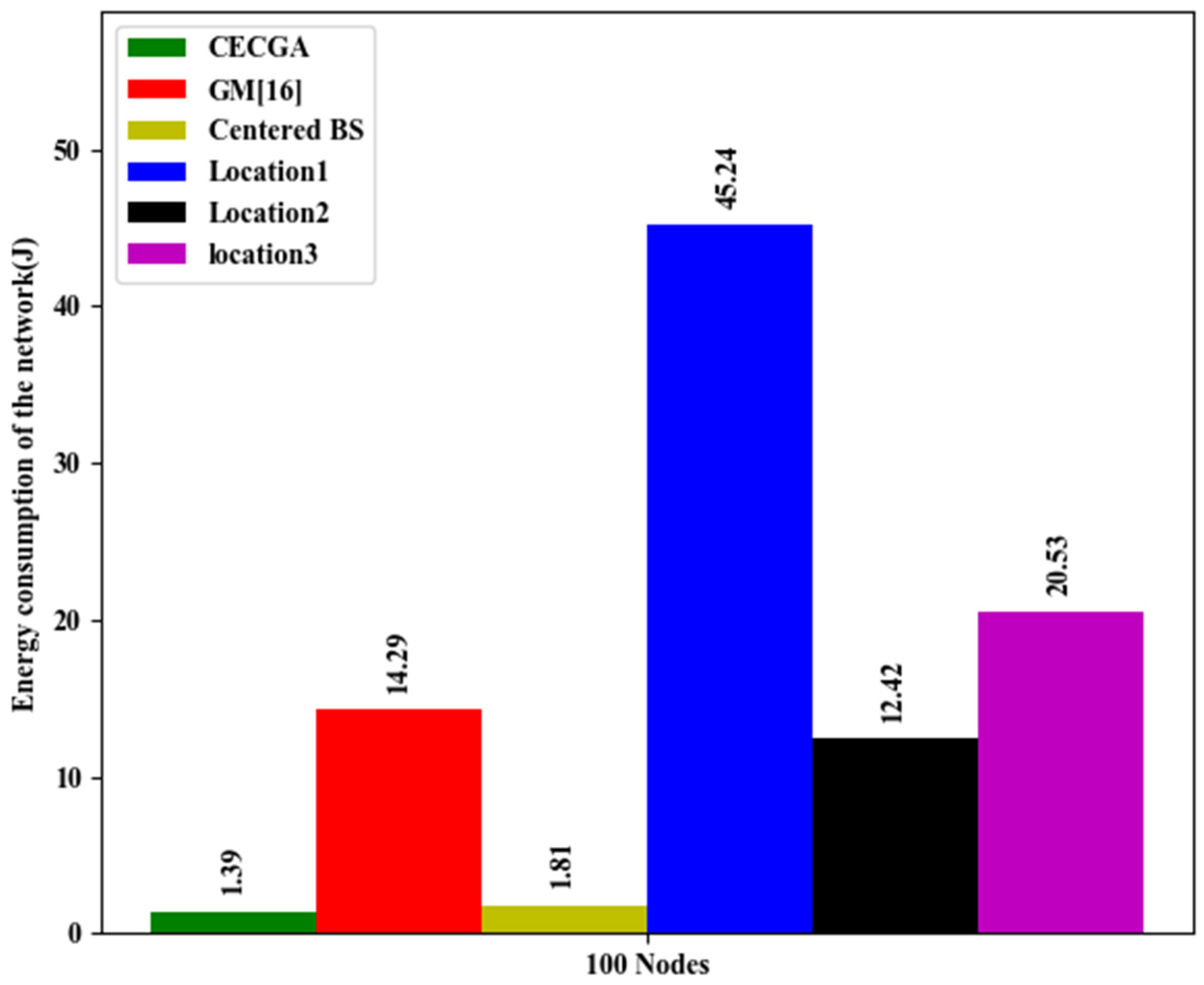
| CECGA (54, 55) | 340.66 |
| GM [16] (22.62, 51.06) | 123.36 |
| Center (50, 50) | 268.42 |
| Location1 (20, 60) | 121.01 |
| Location2 (30, 45) | 153.76 |
| Location3 (50, 20) | 131.18 |
| CECGA | SGA | SEGA | ||||||||||||||||
|---|---|---|---|---|---|---|---|---|---|---|---|---|---|---|---|---|---|---|
| Gen | Eval | f_opt | f_avg | f_std | f_min | f_max | Eval | f_opt | f_avg | f_std | f_min | f_max | Eval | f_opt | f_avg | f_std | f_min | f_max |
| 0 | 20 | 0.001592 | 0.000991 | 0.000137 | 0.000779823 | 0.00129856 | 20 | 0.001599 | 0.00106 | 0.000231 | 0.000538176 | 0.00145834 | 20 | 0.001611 | 0.00105 | 0.000189 | 0.000494423 | 0.0013418 |
| 20 | 400 | 0.001592 | 0.00118 | 0.000013 | 0.000803815 | 0.00152671 | 420 | 0.001599 | 0.00123 | 0.000263 | 0.00039185 | 0.0015674 | 420 | 0.001611 | 0.00152 | 0.000226 | 0.00150538 | 0.00155114 |
| 40 | 780 | 0.001588 | 0.0012 | 0.0000109 | 0.00153004 | 0.00153142 | 820 | 0.001599 | 0.00124 | 0.000251 | 0.000639105 | 0.0015674 | 820 | 0.001611 | 0.00155 | 0.000251 | 0.000813745 | 0.00158232 |
| 60 | 1160 | 0.001582 | 0.00116 | 0.0000103 | 0.000651205 | 0.00150018 | 1220 | 0.001577 | 0.00126 | 0.000185 | 0.000845623 | 0.0015768 | 1220 | 0.001593 | 0.00156 | 0.00026 | 0.00154934 | 0.00158232 |
| 80 | 1540 | 0.001572 | 0.00118 | 0.00000733 | 0.000680588 | 0.0014894 | 1620 | 0.001577 | 0.00122 | 0.00021 | 0.000797963 | 0.0015768 | 1620 | 0.001582 | 0.00157 | 0.000273 | 0.00156169 | 0.00158232 |
| 100 | 1920 | 0.001572 | 0.00129 | 0.00000728 | 0.000888408 | 0.00152439 | 2020 | 0.001577 | 0.0013 | 0.000117 | 0.0010625 | 0.00159345 | 2020 | 0.001582 | 0.00157 | 0.000186 | 0.00156169 | 0.00158232 |
| 120 | 2300 | 0.001367 | 0.00128 | 0.00000643 | 0.000948841 | 0.00158649 | 2420 | 0.001567 | 0.00131 | 0.000259 | 0.000766973 | 1.61124 | 2420 | 0.001582 | 0.00158 | 0.000206 | 0.0015674 | 0.00158784 |
| 140 | 2680 | 0.001251 | 0.00119 | 0.00000359 | 0.000890643 | 0.00146985 | 2820 | 0.001567 | 0.00124 | 0.000164 | 0.000867219 | 0.00161124 | 2820 | 0.001567 | 0.00158 | 0.000236 | 0.00157919 | 0.00159205 |
| 150 | 2851 | 0.000012 | 0.00125 | 0.00000328 | 0.000822922 | 0.00151509 | 3000 | 0.001058 | 0.0013 | 0.000168 | 0.00092423 | 0.00161124 | 3000 | 0.001042 | 0.00158 | 0.000249 | 0.00158232 | 0.00159205 |
Publisher’s Note: MDPI stays neutral with regard to jurisdictional claims in published maps and institutional affiliations. |
© 2021 by the authors. Licensee MDPI, Basel, Switzerland. This article is an open access article distributed under the terms and conditions of the Creative Commons Attribution (CC BY) license (https://creativecommons.org/licenses/by/4.0/).
Share and Cite
Mukase, S.; Xia, K.; Umar, A. Optimal Base Station Location for Network Lifetime Maximization in Wireless Sensor Network. Electronics 2021, 10, 2760. https://doi.org/10.3390/electronics10222760
Mukase S, Xia K, Umar A. Optimal Base Station Location for Network Lifetime Maximization in Wireless Sensor Network. Electronics. 2021; 10(22):2760. https://doi.org/10.3390/electronics10222760
Chicago/Turabian StyleMukase, Sandrine, Kewen Xia, and Abubakar Umar. 2021. "Optimal Base Station Location for Network Lifetime Maximization in Wireless Sensor Network" Electronics 10, no. 22: 2760. https://doi.org/10.3390/electronics10222760
APA StyleMukase, S., Xia, K., & Umar, A. (2021). Optimal Base Station Location for Network Lifetime Maximization in Wireless Sensor Network. Electronics, 10(22), 2760. https://doi.org/10.3390/electronics10222760