Modified Finite-Difference Time-Domain Method for Hertzian Dipole Source under Low-Frequency Band

Abstract

In this paper, a modified finite-difference time-domain (FDTD) method is proposed for the rapid analysis of a Hertzian dipole source in the low-frequency band. The FDTD technique is one of the most widely used methods for interpreting high-resolution problems such as those associated with the human body. However, this method has been difficult to use in the low-frequency band as the required number of iterations has increased significantly in such cases. To avoid this problem, FDTD techniques using quasi-static assumptions in low-frequency bands were used. However, this method was applied only to plane wave excitation, making it difficult to apply to near-field problems. Therefore, a modified approach is proposed, involving the application of the FDTD technique with a quasi-static approximation to an electric and magnetic dipole problem. The results when using the proposed method are in good agreement with those from a theoretical solution. An example of comparison with the standard FDTD method is shown for illustrating the proposed method’s performance.

1. Introduction

Previous research on the adverse effects of electromagnetic waves has been mainly conducted in the extremely low-frequency band for power transmission lines and the high-frequency band for problems such as mobile phones. Recently, many types of devices have been developed using an intermediate frequency band in the fields of wireless information and wireless power transmission (WPT) [1,2]. As an example of WPT, on-line electric vehicle is being used as an on-campus shuttle bus and is about to be commercialized. The interest in electromagnetic field (EMF) hazards is also increasing due to the undesirable EMF generated from such devices. Therefore, the WHO recommends research on the effects of electromagnetic waves in the intermediate frequency band on the human body [3].

Research on the effects of electromagnetic waves on the human body is carried out through measurement, mechanics, and numerical analysis. Among them, the numerical analysis method is widely used in various subjects because it can be used without limitation, unlike other methods. Specifically, the finite-difference time-domain (FDTD) technique is the most widely used method because it does not perform matrix calculations when calculating complex problems such as high-precision whole-body voxel human models [4].

However, the method is difficult to use under low-frequency, as the number of required iterations is increased in such cases. Several methods have been studied for the use of FDTD techniques at low frequencies but were mainly applicable to incident magnetic field problems using Faraday’s Law [5,6,7,8]. However, Ref. [9] provides the results showing that even in the intermediate frequency band, the incident electric field is not always ignored.

The quasi-static FDTD (QS-FDTD) method utilizes a ramp source to successfully extend FDTD to a low-frequency band [10]. Nevertheless, this method has been mainly used in the study of low-frequency problems only for plane wave sources. The authors in [11] provide the results of induced current distributions assuming that the electromagnetic field radiated by the WPT system is a plane wave. The electromagnetic field distribution is, however, dissimilar concerning a plane wave in the near-field interpretation. Generally, the field distribution is broadly similar to a magnetic dipole when a magnetic field is dominant, such as in a WPT system. The authors in [12] proposed a modified QS-FDTD based on the surface equivalence principle to deal with incident electric and magnetic problems. Although this method also addresses the problems for a Hertzian dipole excitation, it is not intuitive to apply as it consists of a two-step process.

Therefore, a modified FDTD method is proposed here to interpret a Hertzian dipole source for a more accurate analysis. The proposed method for the analysis of various simulations can consider both the case where the electric field or the magnetic field is dominant. In this study, the proposed method is verified using a dielectric sphere model with a theoretical solution. In addition, the results are compared with those of the conventional FDTD method to demonstrate its applicability to actual problems. Finally, the accuracy and analysis speed of the proposed method were examined.

2. Proposed Method

The quasi-static approximation (QSA) can be applied when the size of the simulation system is more than 10 times smaller than the wavelength and satisfies the following condition:

$$\left|\sigma +j\omega \epsilon \right|\gg \omega {\epsilon }_0$$

(1)

where σ and ε are the conductivity and permittivity of the dielectric object, respectively, ω is the radian frequency, and ε₀ is the permittivity of the free space [5]. This approximation is often applied up to a few tens of megahertz [13]. In particular, there is research showing that QSA can be applicable up to 10 MHz in relation to the human body analysis [9]. In [9], the applicable frequency range may be slightly reduced in the actual human model since the limit of the QSA was examined with a dielectric sphere of radius 0.1 m. There have been various studies comparing the limitation of the modified FDTD methods using QSA due to changes in mesh size [12] and frequency [9], or complex realistic human body models with other analysis methods [14,15].

The QS-FDTD method has taken advantage of the fact that the phase is predictable. The phase of the field exterior to the object is identical to that of the incident field, whereas the interior field is the first-order field of the incident field. Therefore, the induced electromagnetic field inside the dielectric material can be quickly calculated by approximating the start of the plane wave source as a ramp function. In the proposed method, the electromagnetic field induced by a Hertzian dipole source is computed by approximating the beginning of the electric and magnetic dipole source as a ramp function. The electromagnetic field inside the dielectric material like a human body induced from the Hertzian dipole is rapidly calculated by applying the quasi-static approximated current.

2.1. Electric Dipole

The electric dipole is arranged in the FDTD technique, as shown in Figure 1. The charge Q is calculated using the Gauss theorem by assuming that uniform spatial discretization is implemented to the FDTD Yee cell, i.e., $\Delta x=\Delta y=\Delta z\equiv \Delta s$ and $E_{x\_face}=E_{y\_face}=E_{z\_face}\equiv E_{face}$ [16]:

$$\begin{array}{ll}Q& =2{\epsilon }_0{E}_{face}\Delta x\Delta y+2{\epsilon }_0{E}_{face}\Delta y\Delta z+2{\epsilon }_0{E}_{face}\Delta z\Delta x\\ & =6{\epsilon }_0{E}_{face}{(\Delta s)}^2\end{array}$$

(2)

The electric field at location of source $(i_{src},j_{src},k_{src})$ is obtained using the following equation by summarizing (2):

$$E_z^n(i_{src},j_{src},k_{src})=-2E_{face}=-\frac{Q}{3{\epsilon }_0{(\Delta s)}^2}$$

(3)

By replacing the charge Q in (3) with the integral of the current $I_s$, the relation of the electric field and current is expressed as:

$$E_z^n(i_{src},j_{src},k_{src})=-\frac{1}{3{\epsilon }_0{(\Delta s)}^2}{\displaystyle \underset{}{\overset{}{\int }}{I}_S(t)\mathrm{dt}}$$

(4)

Therefore, we can get that:

$$I_S(t)=-3{\epsilon }_0{(\Delta s)}^2\frac{\partial }{\partial t}{E}_z^n(t)$$

(5)

The FDTD update equation for the electric dipole is expressed as:

$$E_z^{n+1}(i_{src},j_{src},k_{src})=E_z^n(i_{src},j_{src},k_{src})+\frac{\Delta t}{\epsilon }\left[\frac{\partial H_y}{\partial x}-\frac{\partial H_x}{\partial y}-J_z\right]$$

(6)

where ε is the permittivity, and current density $J_z$ is expressed as:

$$J_z=\frac{I_S(t)\cdot \Delta z}{\Delta x\Delta y}$$

(7)

The $J_z$ used in the proposed method is replaced with ramp function and changed to start smoothly to suppress high-frequency contamination as follows:

$$J_z=\{\begin{array}{cc}0& -\infty <t<t_0\\ \frac{\left(t-\left(\frac{\tau }{\pi }\right)\sin \left(\frac{\pi t}{\tau }\right)\right)}{2}& t_0<t<\tau \\ t-\left(\frac{\tau }{2}\right)& t>\tau \end{array}$$

(8)

where $\tau$ is constant for replication functional behavior of the $J_z$ [10].

2.2. Magnetic Dipole

The magnetic dipole is converted into a square loop of the FDTD Yee cell-aligned current $I_s(t)$ having the same magnetic moment, as shown in Figure 2 [17].

The FDTD update equation for the magnetic dipole is expressed as:

$$E_x^{n+1}(i_{src},j_{src},k_{src})=E_x^n(i_{src},j_{src},k_{src})+\frac{\Delta t}{\epsilon }\left[\frac{\partial H_z}{\partial y}-\frac{\partial H_y}{\partial z}-J_s\right]$$

(9)

$$E_y^{n+1}(i_{src},j_{src},k_{src})=E_y^n(i_{src},j_{src},k_{src})+\frac{\Delta t}{\epsilon }\left[\frac{\partial H_x}{\partial z}-\frac{\partial H_z}{\partial x}-J_s\right]$$

(10)

where uniformly distributed over the cross-section of FDTD Yee cell current density $J_s$ is derived from the current $I_s(t)$:

$$J_s(t)=\frac{I_S(t)}{\Delta s^2}$$

(11)

After that, the process is like electric dipole analysis.

3. Results and Discussion

The induced electric field from Hertzian dipole excitation inside a dielectric sphere is calculated to verify the proposed method. The standard FDTD formulation and code used in this paper are described in [18], and the proposed method was modified by applying a quasi-static approximation to the above FDTD formulation.

Table 1. Simulation parameters.

Parameter	Value
Target frequency	1 MHz
Total number of FDTD cells	40 × 40 × 40
Cell size	1 cm
Source excitation location	20, 10, 20
Sphere center location	20, 25, 20
Sphere conductivity	0.3
Sphere radius	5 cm
Total number of iterations	600

represents the simulation parameters used in the analysis.

3.1. Comparison Results of Hertzian Electric Dipole Excitation

The analytic electric field induced inside the dielectric sphere can be obtained by the boundary value problem based on the assumption that the current distribution is known. The dynamic Green’s function is a method of calculating this problem. As shown in Figure 3, when the sphere is located at its origin, the electric field derived from the Hertzian electric dipole located at $r^{\prime }=b$, $\theta =0^{°}$, and $\varphi =0^{°}$ is as follows:

$$\overrightarrow{E_e^{}}(\overrightarrow{R^{\prime }})=-\frac{\omega k_1\mu C_e}{4\pi }{\displaystyle \sum _{n=1}^{\infty }\frac{2n+1}{n(n+1)}}\left(c_n^{(1)}{h}_n({\rho }_3)\overline{M_{o1n}}(k_2)+d_n^{(1)}\frac{{\left[{\rho }_3{h}_n({\rho }_3)\right]}^{\prime }}{{\rho }_3}\overline{N_{e1n}}(k_2)\right)$$

(12)

where in $\mu$ is permeability of free space, $h_n$ is spherical Hankel function, $\overline{M}$ and $\overline{N}$ are solutions of the homogeneous vector wave equation, ${\rho }_3=k_{1}b$, and the coefficients are expressed as:

$$c_n^{(1)}=\frac{{\left[{\rho }_1{h}_n({\rho }_1)\right]}^{\prime }{j}_n({\rho }_1)-{\left[{\rho }_1{j}_n({\rho }_1)\right]}^{\prime }{h}_n({\rho }_1)}{{\left[{\rho }_3{h}_n({\rho }_3)\right]}^{\prime }{j}_n({\rho }_2)-{\left[{\rho }_2{j}_n({\rho }_2)\right]}^{\prime }{h}_n({\rho }_1)}$$

(13)

$$d_n^{(1)}=\frac{\sqrt{{\epsilon }_r}{\left[{\rho }_1{h}_n^{(1)}({\rho }_1)\right]}^{\prime }{j}_n({\rho }_1)-\sqrt{{\epsilon }_r}{\left[{\rho }_1{j}_n({\rho }_1)\right]}^{\prime }{h}_n({\rho }_1)}{{\epsilon }_r{\left[{\rho }_1{h}_n({\rho }_1)\right]}^{\prime }{j}_n({\rho }_2)-{\left[{\rho }_2{j}_n({\rho }_2)\right]}^{\prime }{h}_n({\rho }_1)}$$

(14)

$k_1$ and $k_2$ represent the propagation constants of regions exterior and interior of the sphere, respectively.

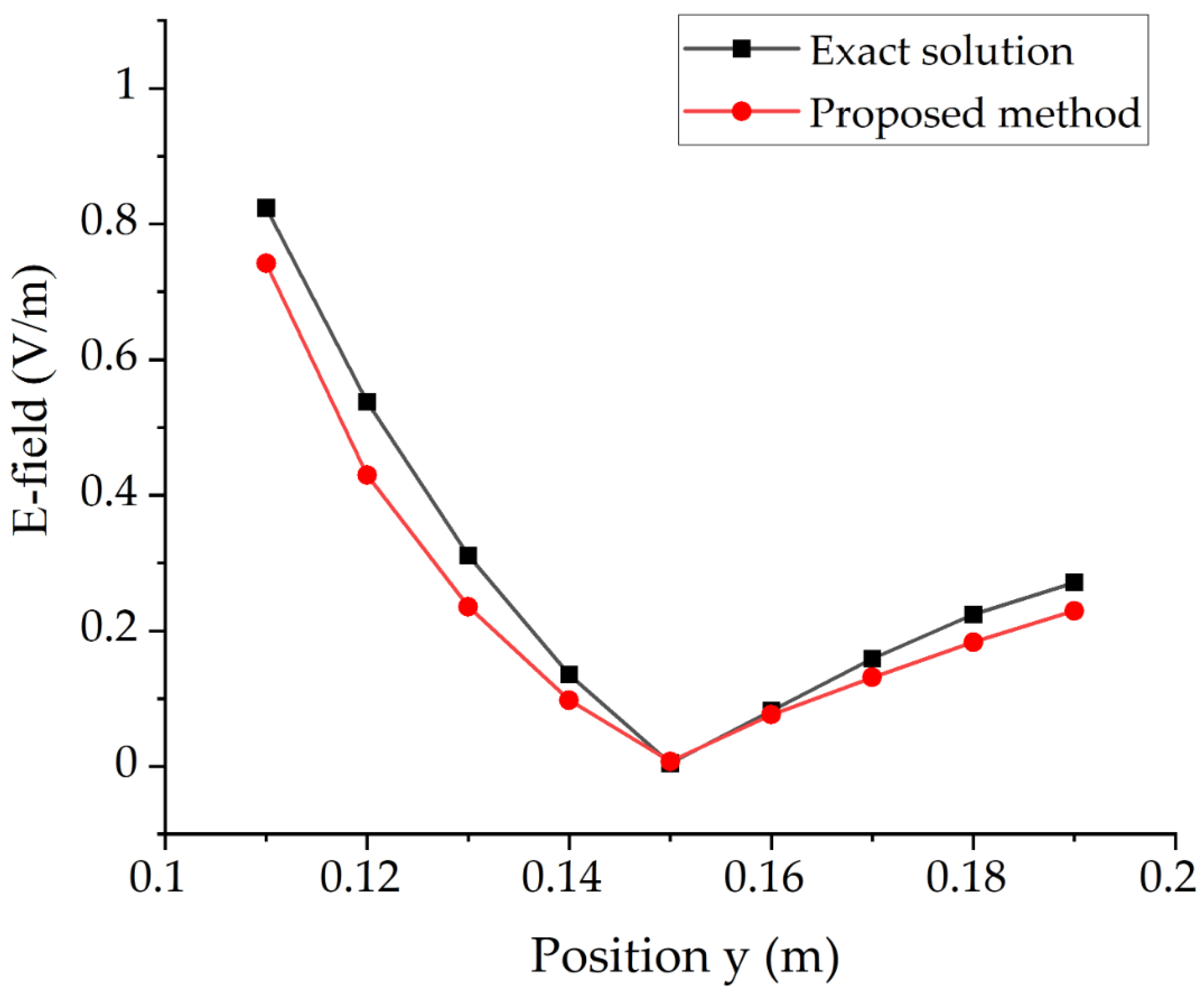
Figure 4 represents the results of comparing the proposed method with the theoretical result.

As shown in Figure 4, the result of the proposed method is consistent with the theoretical result.

3.2. Comparison Results of Hertzian Magnetic Dipole Excitation

The electric field induced inside the sphere from the Hertzian magnetic dipole is expressed as:

$$\overrightarrow{E_m^{}}(\overrightarrow{R^{\prime }})=\frac{i\omega k_1\mu C_m}{4\pi {\eta }_1}{\displaystyle \sum _{n=1}^{\infty }\frac{2n+1}{n(n+1)}}\left(c_n^{(1)}\frac{{\left[{\rho }_3{h}_n({\rho }_3)\right]}^{\prime }}{{\rho }_3}\overline{M_{o1n}}(k_2)-d_n^{(1)}{h}_n({\rho }_3)\overline{N_{e1n}}(k_2)\right)$$

(15)

where, ${\eta }_1=\sqrt{\frac{{\mu }_1}{{\epsilon }_1}}$ is the intrinsic impedance of free space, and the other variables are the same as those used in the Hertzian electric dipole problem.

Figure 5 shows the results of comparing the proposed method with the theoretical result.

As with the Hertzian electric dipole analysis, it can be confirmed that the proposed method is in good agreement with the theoretical results.

3.3. Comparison of the Proposed Method with Standard FDTD Thechnique

To explain the performance of the proposed method, it was compared with the standard FDTD technique used for general problems without theoretical solutions. Analysis objects and variables are the same as those used above. Two-dimensional cross-sectional electric field distributions in the plane z = 0 are presented in Figure 6 and Figure 7 from a Hertzian electric and magnetic dipole excitation, respectively. The comparison of electric field distribution results is summarized in

Table 2. Induced electric field comparisons from Hertzian dipole excitation.

Difference (%)	Plane x = 0	Plane y = 0	Plane z = 0
Hertzian electric dipole	2.34	2.53	2.61
Hertzian magnetic dipole	3.54	3.62	3.24

for each cross-section, which is made based on differences as follows:

$$\mathrm{Difference}=\frac{{\displaystyle \sum _{m=1}^n\left|\frac{\mathrm{Standard}\mathrm{FDTD}-\mathrm{Proposed}\mathrm{method}}{\mathrm{Proposed}\mathrm{method}}\right|}\cdot 100}{n}$$

(16)

Since it is a comparison of numerical analysis methods, it was described as a difference rather than an error.

The number of iterative calculations required for one cycle analysis of a standard FDTD technique is as follows:

$$N=\frac{\sqrt{n}\cdot c_0}{frequency\cdot \Delta x}$$

(17)

where in, $n$ is the dimension of the simulation, $c_0$ is the speed of light, and $\Delta x$ is the mesh size [18].

Three periods are simulated because standard FDTD requires a few periods for convergence. This requires nearly 180,000 iterations; however, the proposed method calculated similar results with only 600 iterations. It takes about 1 h 53 min, and 22 s, respectively, for two methods to complete the analysis with an Intel(R) CPU i5-10400 processor running at 2.90 GHz. In addition, the proposed method converges rapidly regardless of changes in the frequency and size of the mesh, whereas the standard FDTD required more iterations when the frequency and size of the mesh are lowered. Therefore, the proposed method can show stronger performance depending on the analysis variables

4. Discussion

In this paper, the QS-FDTD method is extended to Hertzian dipole source excitation problems. The method is verified through a theoretical solution and the efficiency of the method is explained by comparing the speed that of the standard FDTD method. The method produced accurate results (within 5%) with very few iterative calculations compared to standard FDTD by simulating the beginning of a Hertzian dipole with a ramp function. The method is expected to be widely used for electromagnetic problems at a low frequency as long as quasi-static approximation is effective. In particular, with the development of various devices using intermediate frequency, we believe that the proposed method will be usefully used to intuitively analyze the problem of this frequency band, which has not been mainly studied for high-resolution human body model analysis before.

References

- Kurs, A.; Karalis, A.; Moffatt, R.; Joannopoulos, J.; Fisher, P.; Soljacic, M. Wireless Power Transfer via Strongly Coupled Magnetic Resonances. Science 2007, 317, 83–86. [Google Scholar] [CrossRef] [PubMed]
- Smith, J. Wirelessly Powered Sensor Networks and Computational RFID; Springer: New York, NY, USA, 2013. [Google Scholar]
- Available online: https://www.who.int/peh-emf/publications/facts/intermediatefrequencies_infosheet.pdf?ua=1 (accessed on 23 September 2021).
- Stavroulakis, P.; Markov, M. Biological Effects of Electromagnetic Fields; Springer: Berlin, Germany, 2003; pp. 187–190. [Google Scholar]
- Gandhi, O.P.; DeFord, J.F.; Kanai, H. Impedence Method for Calculation of Power Deposition Patterns in Magnetically Induced Hyperthermia. IEEE Trans. Biomed. Eng. 1984, 31, 644–651. [Google Scholar] [CrossRef] [PubMed]
- DeFord, J.; Gandhi, O. An Impedance Method to Calculate Currents Induced in Biological Bodies Exposed to Quasi-Static Electromagnetic Fields. IEEE Trans. Electromagn. Compat. 1985, EMC-27, 168–173. [Google Scholar] [CrossRef]
- Davey, K.; Cheng, C.; Epstein, C. Prediction of magnetically induced electric fields in biological tissue. IEEE Trans. Biomed. Eng. 1991, 38, 418–422. [Google Scholar] [CrossRef] [PubMed]
- Dawson, T.; De Moerloose, J.; Stuchly, M. Comparison of magnetically induced elf fields in humans computed by FDTD and scalar potential FD codes. In Proceedings of the 1996 Symposium on Antenna Technology and Applied Electromagnetics, Montreal, QC, Canada, 6–9 August 1996; pp. 443–446. [Google Scholar]
- Park, S.; Wake, K.; Watanabe, S. Calculation Errors of the Electric Field Induced in a Human Body Under Quasi-Static Approximation Conditions. IEEE Trans. Microw. Theory Tech. 2013, 61, 2153–2160. [Google Scholar] [CrossRef]
- De Moerloose, J.; Dawson, T.W.; Stuchly, M.A. Application of the finite difference time domain algorithm to quasi-static field analysis. Radio Sci. 1997, 32, 329–341. [Google Scholar] [CrossRef]
- Song, H.-J.; Shin, H.; Lee, H.-B.; Yoon, J.-H.; Byun, J.-K. Induced Current Calculation in Detailed 3-D Adult and Child Model for the Wireless Power Transfer Frequency Range. IEEE Trans. Magn. 2014, 50, 1041–1044. [Google Scholar] [CrossRef]
- Kim, M.; Park, S.; Jung, H.-K. An advanced numerical technique for a quasi-static electromagnetic field simulation based on the finite-difference time-domain method. J. Comput. Phys. 2018, 373, 917–923. [Google Scholar] [CrossRef]
- Kaune, W.; Guttman, J.; Kavet, R. Comparison of coupling of humans to electric and magnetic fields with frequencies between 100 Hz and 100 kHz. Bioelectromagnetics 1997, 18, 67–76. [Google Scholar] [CrossRef]
- Kim, M.; Park, S.; Jung, H.-K. Numerical Method for Exposure Assessment of Wireless Power Transmission under Low-Frequency Band. J. Magn. 2016, 21, 442–449. [Google Scholar] [CrossRef][Green Version]
- Park, S.; Kim, M. Numerical Exposure Assessment Method for Low Frequency Range and Application to Wireless Power Transfer. PLoS ONE 2016, 11, e0166720. [Google Scholar] [CrossRef]
- Costen, F.; Berenger, J.-P.; Brown, A. Comparison of FDTD Hard Source With FDTD Soft Source and Accuracy Assessment in Debye Media. IEEE Trans. Antennas Propag. 2009, 57, 2014–2022. [Google Scholar] [CrossRef]
- Pontalti, R.; Nadobny, J.; Wust, P.; Vaccari, A.; Sullivan, D. Investigation of static and quasi-static fields inherent to the pulsed FDTD method. IEEE Trans. Microw. Theory Tech. 2002, 50, 2022–2025. [Google Scholar] [CrossRef]
- Sullivan, D. Electromagnetic Simulation Using the FDTD Method; IEEE Press: New York, NY, USA, 2000; pp. 1–4. [Google Scholar]