A Learning Control Method of Automated Vehicle Platoon at Straight Path with DDPG-Based PID

Abstract

Cooperative adaptive cruise control (CACC) has important significance for the development of the connected and automated vehicle (CAV) industry. The traditional proportional integral derivative (PID) platoon controller adjustment is not only time-consuming and laborious, but also unable to adapt to different working conditions. This paper proposes a learning control method for a vehicle platooning system using a deep deterministic policy gradient (DDPG)-based PID. The main contribution of this study is automating the PID weight tuning process by formulating this objective as a deep reinforcement learning (DRL) problem. The longitudinal control of the vehicle platooning is divided into upper and lower control structures. The upper-level controller based on the DDPG algorithm can adjust the current PID controller parameters. Through offline training and learning in a SUMO simulation software environment, the PID controller can adapt to different road and vehicular platooning acceleration and deceleration conditions. The lower-level controller controls the gas/brake pedal to accurately track the desired acceleration and speed. Based on the hardware-in-the-loop (HIL) simulation platform, the results show that in terms of the maximum speed error, for the DDPG-based PID controller this is 0.02–0.08 m/s less than for the conventional PID controller, with a maximum reduction of 5.48%. In addition, the maximum distance error of the DDPG-based PID controller is 0.77 m, which is 14.44% less than that of the conventional PID controller.

1. Introduction

Connected and automated vehicles (CAVs) are an important development direction for the automobile industry. They are not only an important way to solve the problems of traffic safety, resource consumption, environmental pollution, etc., but are also the core element of establishing an intelligent transportation system. Cooperative adaptive cruise control (CACC) based on on-board sensors and vehicle-to-vehicle (V2V) and/or infrastructure-to-vehicle (I2V) communication has become a hot spot in the research of intelligent vehicles [1,2]. Through vehicle-to-everything (V2X) communication, this mode can receive the dynamic information of the surrounding environment in real-time and improve driving safety [3,4]. Simultaneously, CACC has a significant influence on improving the road capacity, reducing fuel consumption, decreasing environment pollution, and so on [5,6,7].

By sharing information among vehicles, a CACC system allows automated vehicles to form platoons and be driven at harmonized speed with smaller constant time gaps between vehicles [8]. CACC plays a positive role in improving the performance of the vehicular platooning system and ensuring the safety of vehicles, so it has attracted wide attention from researchers. Previous methods for CACC include proportional integral derivative (PID) control [9,10], sliding mode control (SMC) [11,12], model predictive control (MPC) [13,14,15], H-Infinity (H∞) control [16,17], etc. Due to the advantages of low complexity and less computation, PID controllers play an important role in the control field. However, the parameters of the PID controller need to be adjusted manually and cannot adapt to different working conditions. The control effect of SMC, MPC, and H∞ methods are closely related to model accuracy, and need a reasonably good model of the system to be controlled. When the model precision is higher, the control effect is better. Nevertheless, due to the complex nonlinear dynamics of the longitudinal movement of the vehicular platooning, it is difficult to establish an accurate model.

In recent years, Google’s DeepMind team has combined deep neural networks with the decision-making capabilities of reinforcement learning to establish a framework for deep reinforcement learning (DRL) [18]. Then the deep deterministic policy gradient (DDPG) algorithm was proposed to realize the control of the continuous action space [19]. In addition, it has achieved good results in the field of automatic driving control [20]. At present, the DRL algorithm is mainly applied to the control of individual vehicles, specifically divided into longitudinal [21,22] and lateral [23,24] motion control. Zhu et al. [21] used real-world driving data for training and proposed a human-like car-following model based on the DDPG algorithm, which has higher accuracy than traditional methods. A lane change model based on DRL was designed, which can achieve more stable, safe, and efficient results by adjusting the reward function [23]. Chen et al. [25] proposed a path tracking control architecture that combines a conventional pure pursuit method and DRL algorithm. It was found that the approach of adding a DRL in parallel improves the performance of a traditional controller under various operating conditions. Zhou et al. [26] proposed a framework for learning the car-following behavior of drivers based on maximum entropy deep inverse reinforcement learning. Aiming at the problem of simple simulation scene setting in the above research, Makantasis et al. [27] established the traffic flow model in SUMO simulation software to train the agent. The car-following and lane-changing behavior integrated model using DDPG was developed and trained in the VISSIM simulation environment [28]. Some studies have tried to apply theory to practice [22], but the DRL algorithm based on a deep neural network is a “black box” model. In other words, the control principle is unknown and has significant uncertainty. The training results depend on the setting of random seeds, which is unstable. This is the reason why the current DRL algorithm is mainly implemented on the simulation platform and is difficult to apply to the real vehicle [29].

The learning controller has the strong ability of discrimination, memory, and self-adjustment. It can adjust its own parameters according to different controlled objects and environmental changes to achieve the best control performances. There are currently three main types of learning control systems: iterative learning control (ILC) [30,31], adaptive control based on neural networks (NN) [32,33], and learning control based on the Markov decision process (MDP) [34,35]. Wang et al. [30] presented a novel learning-based cruise controller for autonomous land vehicles (ALVs). The controller consists of a time-varying proportional-integral (PI) module and an actor-critic learning control module. Lu et al. [36] designed a personalized driving behavior learning system based on neural reinforcement learning (NRL), which utilized data collected by on-board sensors to learn the driver’s longitudinal speed control characteristics. Combining DRL with traditional control methods has been a research hotspot in recent years. It takes advantage of the self-learning and self-tuning abilities of DRL. Moreover, it uses the traditional controller to ensure the stability of the system. The learning-based predictive control (LPC) method using the actor-critic framework was proposed, which was shown to be asymptotically stable in the sense of Lyapunov [37]. Ure et al. [38] developed a reinforcement learning framework for automated weight tuning for MPC-based adaptive cruise control (ACC) systems. This approach significantly shortens the exhausting manual weight tuning process.

In summary, researchers in different fields have already completed numerous works in the longitudinal motion control of vehicular platooning, but there still exist some deficiencies as follows. (1) The vehicular platooning controller is difficult to adapt to various working conditions and controller parameters must be set manually by professional engineers (e.g., PID). The existing controllers such as MPC, LQR, and H∞ need a high-precision controlled object model. However, this knowledge is very difficult to obtain. (2) Neural networks and their derived controllers belong to the scope of supervised machine learning, which can only imitate the parameter adjustment strategies of expert demonstrations, but not necessarily the optimal control effect. Another issue is that their generalization ability also needs to be proved. (3) The end-to-end learning method performs well in an autonomous driving simulation environment, but its interpretability is poor, and there is little literature to analyze the stability of the control system. The vehicular platooning has complex nonlinearity, so the actual control effect cannot be guaranteed.

In view of the above problems, a learning control method that uses DDPG-based PID for longitudinal motion control of vehicular platooning is proposed in this paper. PID controllers are the most commonly used for industrial applications due to their simplicity in structure and robustness in performance. However, the traditional PID adjustment is not only time-consuming and laborious, but also unable to adapt to different working conditions. Therefore, we proposed a novel control strategy of vehicular platooning using DDPG-based PID to solve this problem. To the best knowledge of the authors, this is the first reported use of DDPG-based PID for vehicular platooning control. The PID controller parameters can be automatically adjusted in real-time according to the state by using a trained DDPG algorithm. Through offline training and learning in a simulation environment, the PID controller can adapt to different road and vehicular platooning acceleration and deceleration conditions. The advantage of this scheme is that the PID controller parameters do not rely on any manual tuning and can better adapt to the change in working conditions. The DDPG-based PID controller eliminates the drawbacks of the traditional PID controller, such as insufficient adaptability, and the difficulty of parameter regulation. In addition, the vehicular platooning system stability is proved by stability theory to ensure safety. Therefore, compared with the traditional PID controller, the DDPG-based PID has stronger robustness. This study is the further development of the learning control method, and provides a new idea for the practical application of DRL algorithm in the industrial field. However, the HIL simulation simplifies the road environment conditions. How to carry out real vehicle experiments to further verify the stability and reliability of a vehicular platoon controller is the focus of the next research in this paper.

The work in this paper is an extension of our previous publication [39]. The remainder of this paper is organized as follows. In Section 2, the architecture of the vehicular platooning control system and a string stability analysis are presented. In Section 3, we illustrate how the problem of vehicular platoon control is formulated as an MDP model. The DDPG-based PID control algorithm is trained in Section 4. In Section 5, the experimental result is presented and in Section 6, the results are analyzed and discussed. Finally, the conclusions and future work outlook are provided in the last section.

2. Methodology

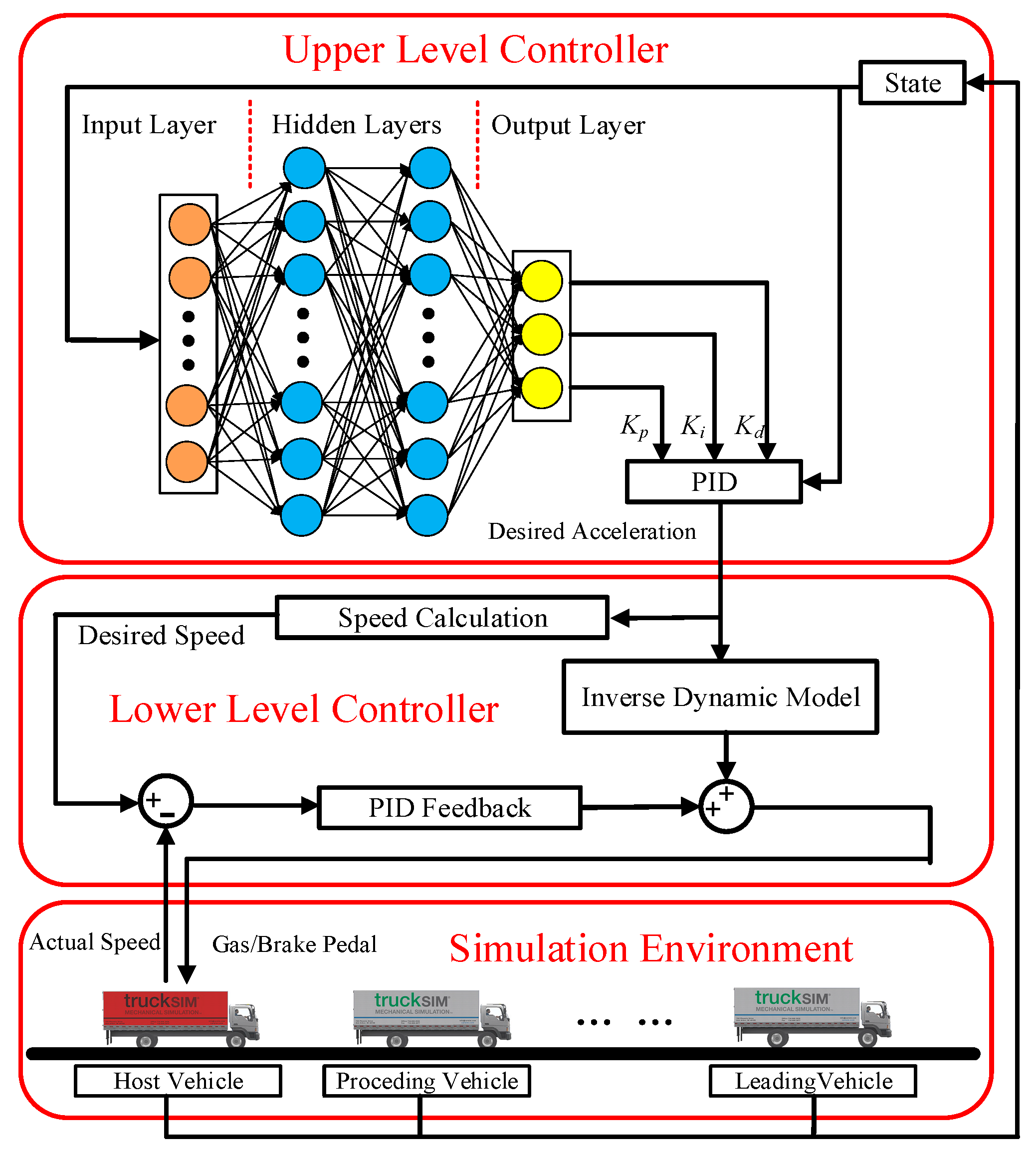
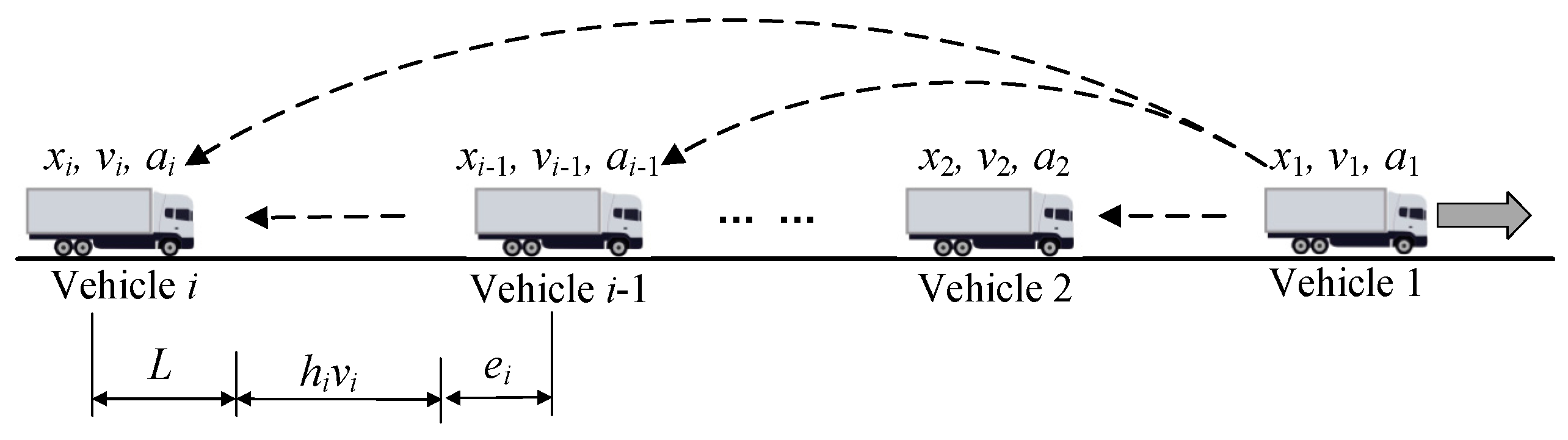
2.1. Vehicle Platoon Architecture

The information topology has an important impact on the stability of vehicular platooning. Currently, the main topologies include the predecessor following (PF) topology, bidirectional (BD) topology, and predecessor-leader following (PLF) topology [40]. In addition, the vehicle spacing control strategies consist of the constant spacing (CS) policy, constant time-gap (CT) policy, and variable time-gap (VT) policy [41]. The PLF topology and CT policy frameworks are applied in this paper to realize the vehicular longitudinal tracking control, as shown in Figure 1.

Based on the hierarchical control structure [42], the upper-level controller receives the state information (such as vehicle position, speed, and acceleration) through communication technology and on-board sensors, and calculates the desired longitudinal acceleration. Then, the lower-level controller controls the gas/brake pedal to accurately track the desired acceleration and speed, with feedforward and feedback control logic. This paper focuses on the upper-level controller; meanwhile, the dynamic models of the vehicle powertrain system and braking system are handled by the lower-level controller. The vehicular platooning control framework is shown in Figure 2. In our system, we assume that the leading vehicle can be maneuvered in real time by automatic or manual driving, and that each vehicle is equipped with a global positioning system (GPS) and on-board sensors, and has V2V communication technology.

2.2. Vehicle Platoon Control

2.2.1. Upper-Level Controller

Using DDPG-based PID, the upper-level controller can adjust the PID controller parameters in real-time according to the state of the vehicular platooning. For a homogeneous vehicle platoon, the longitudinal model of the ith vehicle is obtained by considering the delay characteristic of the vehicle actuator as [43]:

$$\begin{array}{c}{\dot{x}}_i(t)=v_i(t)\\ {\dot{v}}_i(t)=a_i(t)\\ {\dot{a}}_i(t)=\frac{1}{\tau }\left[u_i(t)-a_i(t)\right]\end{array}$$

(1)

where x_i(t), v_i(t), a_i(t), u_i(t) represent the position, velocity, acceleration, and desired acceleration of the center of gravity, respectively; τ is the first-order lag of the vehicle actuator. The platoon consists of N vehicles (or nodes), i.e., a leader (indexed as 1) and N−1 followers (indexed by i accordingly).

For the ith vehicle, we can define the distance ε_i,i−1(t) and distance error e_i,i−1(t) between the ith and (i−1)th (preceding) vehicle as:

$$\{\begin{array}{l}{\epsilon }_{i,i-1}(t)=x_{i-1}-x_i\\ e_{i,i-1}(t)={\epsilon }_{i,i-1}(t)-x_d\end{array}$$

(2)

where x_d represents the desired distance between neighboring vehicles with x_d = v_ih + L; h is the constant-time headway; and L is the safety distance, which contains the length of the vehicle body.

Similarly, we can also obtain:

$$\{\begin{array}{l}{\epsilon }_{i,1}(t)=x_1-x_i\\ e_{i,1}\left(t)={\epsilon }_{i,1}\right(t)-(i-1)x_d\end{array}$$

(3)

where ε_i,1(t), e_i,1(t) denote the distance and distance error between the ith vehicle and the leading vehicle, respectively.

For the PLF topology, the distance error of the ith vehicle consists of two parts, i.e.,

$${\delta }_i(t)={\lambda }_1{e}_{i,i-1}(t)+{\lambda }_2{e}_{i,1}(t)$$

(4)

where λ₁, λ₂ are weight coefficients of e_i,i−1(t) and e_i,1(t), which are bounded with λ₁ + λ₂ = 1, 0 < λ₁ < 1 and 0 < λ₂ < 1.

The controllers are distributed in each vehicle, and each controller can use information for the preceding vehicle and leading vehicle. Based on (4), we can obtain u_i(t) as:

$$u_i(t)=K_p{\dot{\delta }}_i(t)+K_i{\displaystyle \int {\dot{\delta }}_i(t)}+K_d{\ddot{\delta }}_i(t)$$

(5)

where K_p, K_i, and K_d are the weight parameters of the PID controller.

Then, the output of the upper-level controller of the ith (i ≥ 2) vehicle is expressed as:

$$u_i={\lambda }_1\left[K_p(v_{i-1}-v_i)+K_i({\epsilon }_i-x_d)+K_d(a_{i-1}-a_i)\right]+{\lambda }_2\left[K_p(v_1-v_i)+K_i\left({\epsilon }_{i,1}-(i-1)x_d\right)+K_d(a_1-a_i)\right]$$

(6)

2.2.2. Lower-Level Controller

The output of the lower controller is throttle opening or brake pressure, which can accurately track the desired acceleration and speed. According to the desired acceleration calculated by (5), the desired speed at the next moment can be expressed as follows:

$$v^{*}(t+1)=v(t)+u_i(t)T_s$$

(7)

where v^*(t + 1), v(t) are desired speed at time t + 1 and actual speed at time t, respectively; u_i(t) is desired acceleration; and T_s denotes the sampling period. The lower controller adopts a feedforward plus feedback control scheme. The feedforward value u_lf(t) is obtained from the longitudinal inverse dynamics model [44], and the feedback value is calculated by the PID feedback control method of speed error. Therefore, the output of the lower-level controller is as follows:

$$u_l(t)=u_{lf}(t)+K_1{v}_e(t)+K_2{\displaystyle {\int }_0^t{v}_e(t)dt}+K_3\frac{d{v}_e(t)}{dt}$$

(8)

where v_e(t) is the deviation between the expected speed and the actual speed; K₁, K₂, and K₃ are positive parameters of controller.

2.2.3. Transfer Function of Distance Error

Based on Equation (1), the longitudinal dynamics of the ith and (i−1)th vehicles can be described by:

$$\{\begin{array}{l}{\dot{a}}_i(t)=\frac{1}{\tau }\left[u_i(t)-a_i(t)\right]\\ {\dot{a}}_{i-1}(t)=\frac{1}{\tau }\left[u_{i-1}(t)-a_{i-1}(t)\right]\end{array}$$

(9)

The time derivative of Equation (2) can be written as:

$${\stackrel{⃛}{e}}_{i,i-1}(t)={\dot{a}}_{i-1}(t)-{\dot{a}}_i(t)$$

(10)

Based on Equations (9) and (10), following equation can be expressed:

$$\begin{array}{ll}\tau {\stackrel{⃛}{e}}_{i,i-1}(t)+a_{i-1}(t)-a_i(t)=& {\lambda }_1{K}_p[(v_{i-2}-v_{i-1})-(v_{i-1}-v_i)]+{\lambda }_2{K}_p[(v_1-v_{i-1})-(v_1-v_i)]\\ & +K_i[{\delta }_{i-1}(t)-{\delta }_i(t)]+{\lambda }_1{K}_d[(a_{i-2}-a_{i-1})-(a_{i-1}-a_i)]+{\lambda }_2{K}_d[(a_1-a_{i-1})-(a_1-a_i)]\end{array}$$

(11)

Then, combining Equations (9)–(11), we can obtain:

$$\tau {\stackrel{⃛}{e}}_{i,i-1}(t)+(k_d+1){\ddot{e}}_{i,i-1}(t)+[K_p+h{K}_i({\lambda }_1+(i-1){\lambda }_2)]{\dot{e}}_{i,i-1}(t)+K_i{e}_{i,i-1}(t)={\lambda }_1{K}_d{\ddot{e}}_{i-1,i-2}(t)+{\lambda }_1{K}_p{\dot{e}}_{i-1,i-2}(t)+{\lambda }_1{K}_i{e}_{i-1,i-2}(t)$$

(12)

According to the Laplace transform on Equation (12), the transfer function of the distance error between neighboring vehicles can be derived as:

$$G(s)=\frac{e_{i,i-1}(s)}{e_{i-1,i-2}(s)}=\frac{{\lambda }_1(K_{p}s+K_i+K_d{s}^2)}{\tau s^3+(K_d+1)s^2+[K_p+h{K}_i({\lambda }_1+(i-1){\lambda }_2)]s+K_i}$$

(13)

2.3. String Stability

According to the definition of string stability, the platoon can be said to be stable when the distance error between neighboring vehicles will not be amplified by the increase in the number of vehicles, i.e., [45]:

$$|G\left(j\omega \right)|=\left|\frac{e_{i,i-1}\left(j\omega \right)}{e_{i-1,i-2}\left(j\omega \right)}\right|<1,\forall \omega >0$$

(14)

Proof. 

Substituting s = jω into Equation (14), we have:

$${\left|G(j\omega )\right|}^2={\left|\frac{e_{i,i-1}(j\omega )}{e_{i-1,i-2}(j\omega )}\right|}^2=\frac{A}{A+B}<1$$

(15)

where

$$\begin{array}{c}A={\lambda }_1{}^2[K_d{}^2{\omega }^4+(K_p{}^2-2K_i{K}_d){\omega }^2+K_i{}^2]\\ B={\tau }^2{\omega }^6+\left\{1+2K_d+(1-{\lambda }_1^2)K_d^2-2\tau \left[K_p+h{K}_i({\lambda }_1+(i-1){\lambda }_2)\right]\right\}{\omega }^4\\ \hspace{1em}\hspace{1em}\hspace{1em}\hspace{1em}\hspace{0.17em}+\left\{{\left[K_p+h{K}_i({\lambda }_1+(i-1){\lambda }_2)\right]}^2-2(1+K_d)K_i+{\lambda }_1^2(2K_i{K}_d-K_p^2)\right\}{\omega }^2+(1-{\lambda }_1^2)K_i^2\end{array}$$

If the condition of Equation (15) is fulfilled, we have B > 0. Let x = ω², then x > 0. Considering τ²ω⁶ > 0, the rest of B can be described by:

$$\begin{array}{ll}f(x)=& \{1+2K_d+(1-{\lambda }_1^2)K_d^2-2\tau [K_p+h{K}_i({\lambda }_1+(i-1){\lambda }_2)]\}{x}^2\\ & +\{{[K_p+h{K}_i({\lambda }_1+(i-1){\lambda }_2)]}^2-2(1+K_d)K_i+{\lambda }_1^2(2K_i{K}_d-K_p^2)\}x+(1-{\lambda }_1^2)K_i^2\end{array}$$

(16)

Then the function f (x) can be rewritten as:

$$f(x)=a{x}^2+bx+c$$

(17)

where

$$\begin{array}{c}a=1+2K_d+(1-{\lambda }_1^2)K_d^2-2\tau \left[K_p+h{K}_i({\lambda }_1+(i-1){\lambda }_1)\right]\\ b={[K_p+h{K}_i({\lambda }_1+(i-1){\lambda }_2)]}^2-2(1+K_d)K_i+{\lambda }_1^2(2K_i{K}_d-K_p^2)\\ c=(1-{\lambda }_1^2)K_i^2\end{array}$$

For a single-variable quadratic function, if given any x > 0, there exists f (x) > 0, which can be divided into the following two cases. Defining γ = λ₁ + (i−1) λ₂, we can compute the sufficient and unnecessary conditions for stability of the platoon as follows:

Case A:

$$\{\begin{array}{l}f(0)>0\\ -\raisebox{1ex}{$b$}\!\left/ \!\raisebox{-1ex}{$2a$}\right.\le 0\\ a>0\end{array}$$

(18)

Then we can derive that:

$$\{\begin{array}{l}(1-{\lambda }_1^2)K_i^2>0\\ {(K_p+h{K}_i\gamma )}^2\le 2(1+K_d)K_i+{\lambda }_1^2(2K_i{K}_d-K_p^2)\\ {(1+K_d)}^2>2\tau (K_p+h{K}_i\gamma )+{\lambda }_1^2{K}_d^2\end{array}$$

(19)

Case B:

$$\{\begin{array}{l}f\left(-\raisebox{1ex}{$b$}\!\left/ \!\raisebox{-1ex}{$2a$}\right.\right)>0\\ -\raisebox{1ex}{$b$}\!\left/ \!\raisebox{-1ex}{$2a$}\right.>0\\ a>0\end{array}$$

(20)

Here, the following equation is obtained from Equation (20):

$$\{\begin{array}{l}4K_i^2(1-{\lambda }_1^2)[{(1+K_d)}^2-{\lambda }_1^2{K}_d^2-2\tau (K_p+h{K}_i\gamma )]>{[{(K_p+h{K}_i\gamma )}^2-2(1+K_d)K_i+{\lambda }_1^2(2K_i{K}_d-K_p^2)]}^2\\ {(K_p+h{K}_i\gamma )}^2>2(1+K_d)K_i+{\lambda }_1^2(2K_i{K}_d-K_p^2)\\ {(1+K_d)}^2>2\tau (K_p+h{K}_i\gamma )+{\lambda }_1^2{K}_d^2\end{array}$$

(21)

If given any parameters K_p, K_i, and K_d meet the requirements of Equation (19) or (21), then the stability of the platoon can be guaranteed. □

3. Design of DDPG-Based PID Vehicle Platoon Controller

3.1. MDP Model for Vehicle Platoon Control

The problem of vehicular platoon control is formulated as an MDP model in this section. In our system, we assume that the environment is fully observable. The states, actions, and the reward function of the MDP are defined as follows.

Choosing an appropriate state space is critical to the convergence of the reinforcement learning algorithm. The selected state information should be related to the motion state of the platoon. According to PLF topology, the state space includes the relative position, relative speed, and relative acceleration between the host vehicle, the preceding vehicle, and the leading vehicle, respectively. At time step t, a set of states s_t consists of six elements, i.e.,

$$s_t=\left\{\Delta a_{i,i-1},\Delta v_{i,i-1},\Delta x_{i,i-1},\Delta a_{i,1},\Delta v_{i,1},\Delta x_{i,1}\right\}$$

(22)

where Δa_i,i−1, Δv_i,i−1, Δx_i,i−1 are relative acceleration, relative speed, and relative position of the host vehicle and the preceding vehicle. Δa_i,1, Δv_i,1, Δx_i,1, denote relative acceleration, relative speed, and relative position of the host vehicle and the leading vehicle, respectively.

In the upper controller, the DDPG algorithm adjusts PID controller parameters in real-time, so the action space is:

$$a_t=\left\{K_p,K_i,K_d\right\}$$

(23)

The goal of reinforcement learning is to find the optimal strategy to maximize the cumulative reward. The design of the reward function needs to consider the following aspects. Firstly, it is necessary to ensure that there is no collision between vehicles, when the vehicular platoon system is traveling. Secondly, the stability of the platoon should be guaranteed, i.e., the relative position among vehicles should be maintained at a reasonable distance. Thirdly, the host vehicle needs to respond quickly, which can follow the motion state of the preceding vehicle. Through the above analysis, the reward functions designed in this paper include the following parts:

$$\begin{array}{c}R=R_1+R_2+R_3+R_4\\ R_1=\{\begin{array}{ll}0& \Delta x_{i,i-1}\ge L\\ -100& \Delta x_{i,i-1}<L\end{array}\\ R_2=-{\omega }_1\left|\Delta v_{i,i-1}\right|\\ R_3={\omega }_2\left(\right|e_{i,i-1}(t-1)|-|e_{i,i-1}(t)\left|\right)-{\omega }_3\left(\left|e_{i,i-1}(t)\right|\right)\\ R_4=\{\begin{array}{cc}0& -3.5\le a_i\le 2\\ {\omega }_4(2-\left|a_i\right|)& a_i>2\\ {\omega }_4(3.5-\left|a_i\right|)& a_i<-3.5\end{array}\end{array}$$

(24)

where ω₁, ω₂, ω₃, ω₄ are the positive weight coefficients of the reward function.

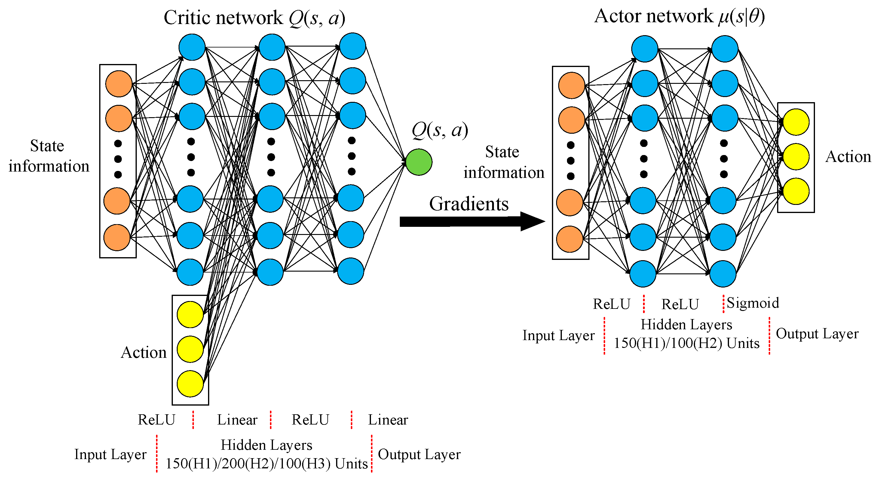
3.2. Structural Design of DDPG Algorithm

In this paper, there is no image as input, so we use a full connection network to construct the DDPG network. The overall structure of the neural network is shown in Figure 3. There are 4 layers in the actor network, including 1 input layer, 1 output layer, and 2 hidden layers. There are 150 and 100 neurons in the hidden layers, which use the rectified linear unit (ReLU) activation function, because it has the advantage of accelerating convergence [46]. The input to the actor network is the state s_t and the output is the action a_t, which is a set of PID controller parameters. The final output layer of the actor network uses 3 sigmoid activation functions to generate continuous action values with a limit of (0, 1).

The critic network takes the state s_t and the action a_t as input, and outputs a scalar Q-value Q(s_t, a_t). The critical network consists of 2 input layers, 1 output layer, and 3 hidden layers containing 150, 200, and 100 hidden units. The ReLU activation function is used in the first and third hidden layers, and linear activation function is used to sum the variable values. It should be noted that the values vary greatly due to the different units of input state variables. In order to eliminate the dimensional influence between the data and improve the training effect, batch normalization is utilized, which can transform the input data into a normal distribution. In addition, the Ornstein–Uhlenbeck process noise is used to explore in order to improve the efficiency of exploration in the inertial system. Other training parameters are listed in

Table 1. Training parameter settings.

Parameter	Meaning	Value
LRA	Learning rate for actor network	0.0001
LRC	Learning rate for critic network	0.001
Update rate	Update rate of target network tau	0.001
BUFFER_SIZE	Reply memory size	100,000
BATCH_SIZE	Batch size	64
ω1, ω2, ω3, ω4	Reward function weight	0.1, 5, 0.05, 1
γ	Discount factor	0.9

.

4. Training of DDPG-Based PID Control Algorithm

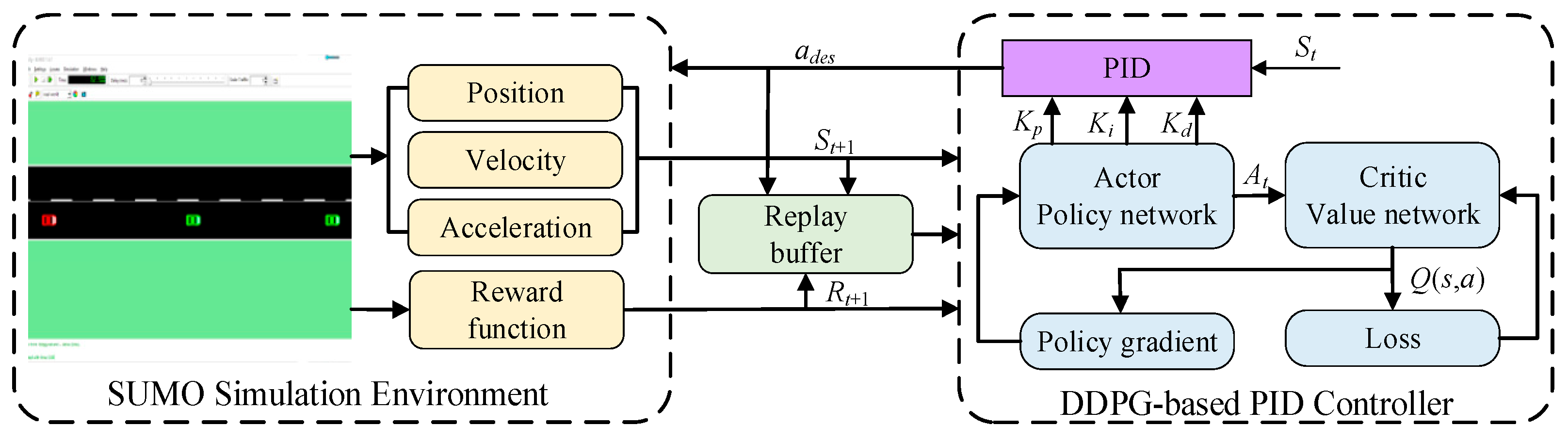
4.1. Training Environment-SUMO

As is shown in Figure 4, a deep reinforcement learning training platform based on SUMO is designed in this paper, which is mainly composed of a SUMO simulator and an external controller Jetson TX2. The vehicle kinematics model and simulation scene are provided by SUMO. Meanwhile, the DDPG-based PID algorithm is written in Python language, stored in the Jetson TX2, and trained according to the simulation data. Considering the vehicle platoon communication structure and actual test conditions, three vehicles are set up to form a platoon driving along the straight road in the SUMO simulator. The first, second, and third vehicles are the leading vehicle, preceding vehicle, and host vehicle (red vehicle in Figure 4), respectively.

During the training process, the dynamic states of the three vehicles in SUMO are transmitted to the DDPG algorithm through traffic control interface (Traci) communication. After data processing, the state s_t is input to both the actor and the critical network, and three PID parameters are output. The movement of the leading vehicle is planned in advance. The preceding vehicle can follow the speed change of the leading vehicle by manually adjusting the PID controller. The whole training process is iterative and cyclic.

4.2. Vehicle Platoon Control Policy Algorithm

The training process of the DDPG-based PID algorithm is divided into two cycles to learn the policy of vehicle platoon longitudinal control, as shown in Algorithm 1. Firstly, the parameters of the actor network and the critical network and replay buffer are initialized. Next, when the external cycle starts to run, the SUMO simulation environment needs to be initialized to obtain the initial state s₁. In the inner cycle, the action a_t is output according to the state s_t, which is the three parameters of the PID controller. Then, the desired acceleration a_des is calculated and implemented in the simulation environment. The reward r_t and new state s_t+1 are observed and saved into the replay buffer. Finally, the training samples are randomly selected from the replay buffer to update the parameters of the actor and critical network.

Algorithm 1. DDPG-based PID algorithm for vehicle platoon longitudinal control
1	Randomly initialize critic network and actor network
2	Initialize target networks and replay buffer
3	for episode = 1, to M do
4	Initialize SUMO simulation environment;
5	Receive initial observation state s1;
6	for step = 1 to T do
7	Select action at based on current actor network and calculate the desired acceleration of host vehicle ades;
8	Execute desired acceleration ades in SUMO simulator and observe reward rt, new state st+1;
9	Save transition (st, at, rt, st+1) into replay buffer;
10	Sample a random batch size of N transitions from replay memory;
11	Update critic by minimizing the loss;
12	Update actor policy using the sampled gradient;
13	Update the target networks;
14	end for
15	end for

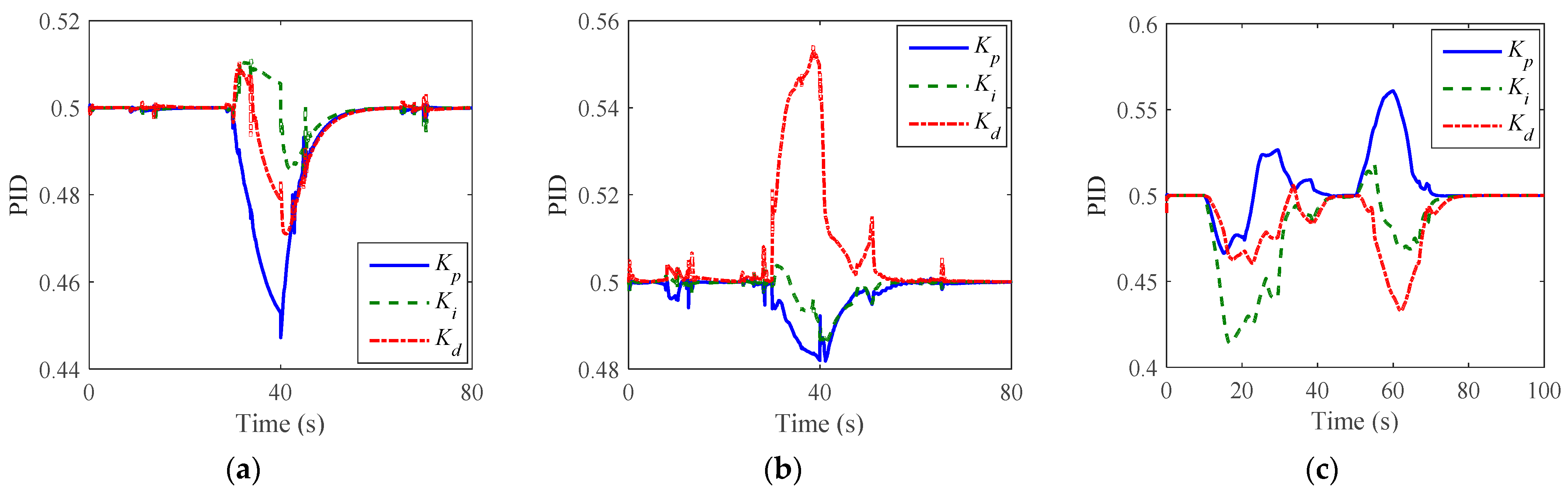
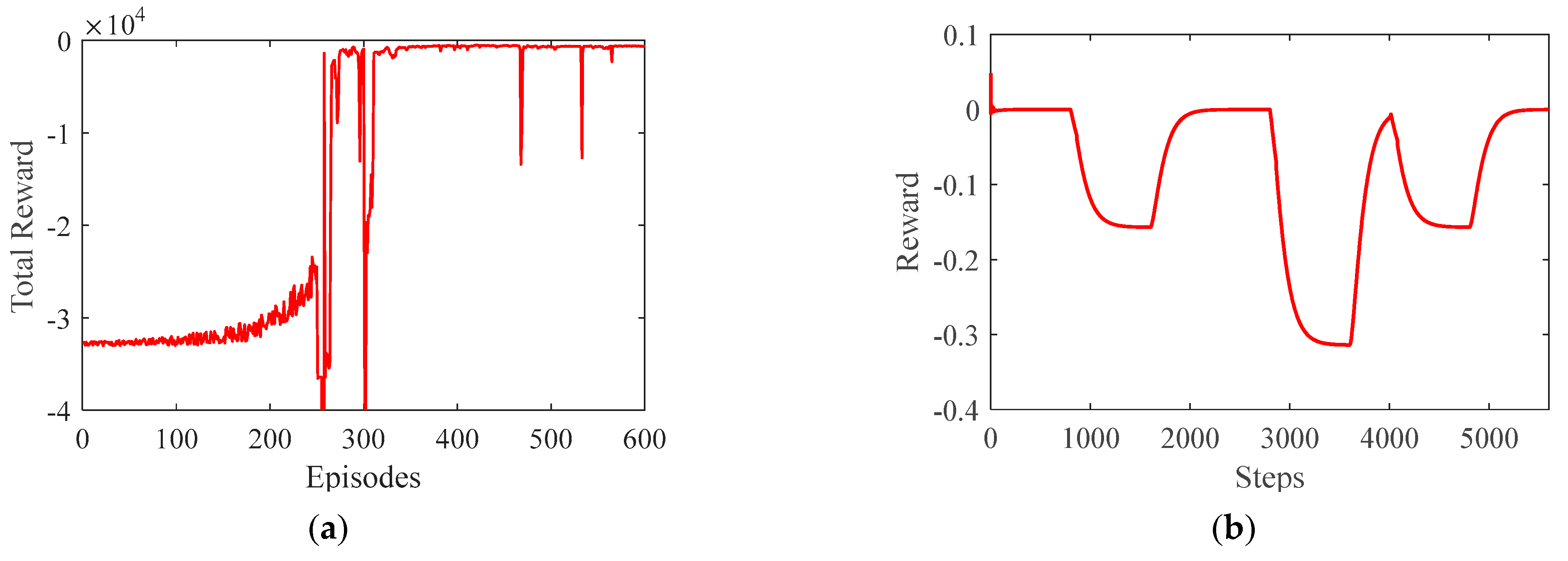
4.3. Algorithm Training Results

The scene of algorithm training should be representative, so the driving cycle including acceleration, cruise, and deceleration is designed in this paper. In this study, the simulation of the dynamic performance of the platoon at different speeds is achieved by setting the speed profile in the leading vehicle. Figure 5 shows the speed and acceleration changes of the leading vehicle. The parameters λ₁ and λ₂ in (4) are 0.5, and the training results are shown in Figure 6.

From Figure 6a–d, we can see that the vehicle using the DDPG-based PID controller can track the leading and preceding vehicle well in the entire movement process. The speed and acceleration change smoothly without overshoot. At the same time, when the leading vehicle begins to accelerate, the platoon takes about 15 s to reach steady state. When the leading vehicle returns to uniform speed, the platoon can reach steady state in about 5 s. The maximum distance error of the vehicle platoon is 0.38 m and the following vehicles can track the changes of the leading vehicle in time.

The DRL agent is trained using the DDPG algorithm for 600 episodes, where each episode starts with the same initial state and lasts for 5600 steps. The total reward per episode and reward per step are shown in Figure 7. The greater the value of the total reward per episode, the better the training performance.

As can be seen from Figure 7a, the cumulative reward per episode value increases with time of training. The algorithm converges after training for 320 episodes and the cumulative reward is about −500. According to Figure 7b and the definition of the reward function, it can be concluded that the maximum reward per step whose value is 0 occurs when the speed and distance deviation between the controlled vehicle and the front vehicle is 0, and the speed changes smoothly. That is to say, when the leading vehicle travels at a constant speed, the whole platoon keeps stable and the reward value is the largest. Due to the CT policy strategy, when the preceding vehicle speed changes, the host vehicle cannot accurately track the desired speed and distance at the same time. Then the reward inevitably appears to be a negative value. In addition, the larger the acceleration, the smaller the reward value will be. However, it can be seen from Figure 7b that the minimum reward value in the training episode is −0.32, which indicates that the model using on the DDPG-based PID platoon control algorithm can reduce the tracking error between the host vehicle and the preceding vehicle as much as possible.

5. Experimental Results

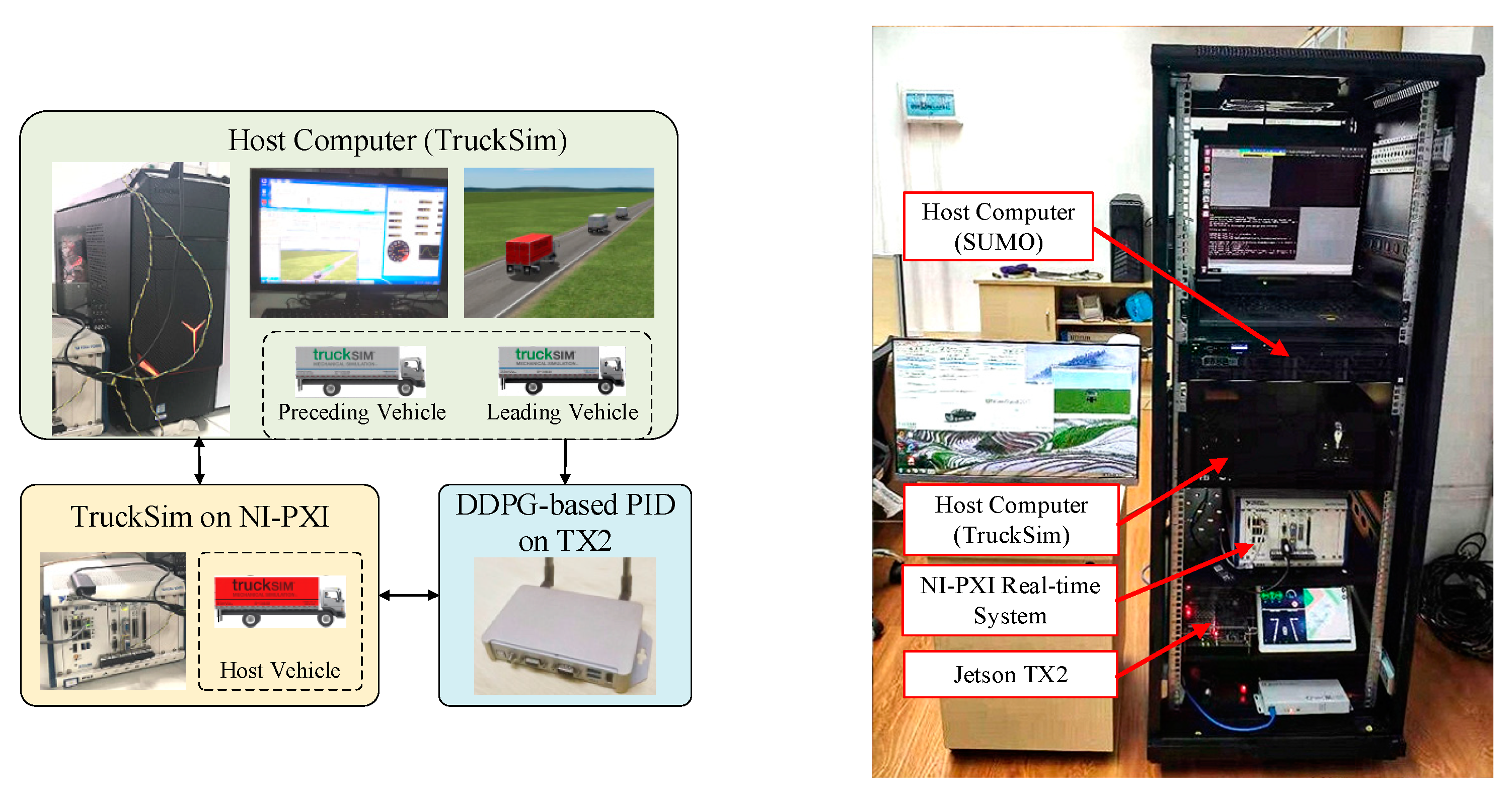
5.1. Design of Hardware-in-the-Loop (HIL) Platform

To validate the effectiveness of the proposed method more realistically, the vehicle dynamic model is introduced to carry out the HIL test, which makes the system closer to the real environment. The platform is mainly composed of TruckSim software, Matlab/Simulink software, external controller Jetson TX2, NI-PXI real-time system, and the host computer, etc. In the simulations, a platoon consists of three trucks with the same structural parameters. The truck model LCF Van model is adapted, whose main dynamic parameters are listed in

Table 2. Main parameters of vehicle LCF Van dynamics.

Parameter	Meaning	Value
m	Mass (kg)	5762
hcg	Height of C.G (m)	1.1
L	Safe distance (m)	5
A	Frontal area (m2)	6.8
Lf/Lr	Front/rear track width (m)	2.030/1.863

.

The vehicular dynamic software Trucksim provides dynamic models of the platoon. The leading vehicle and the preceding vehicle are controlled by Matlab/Simulink in the host computer. The platoon controller obtains the state information through a CAN bus and outputs the control signal to control the host vehicle in NI-PXI. The overall architecture of the HIL platform is shown in Figure 8.

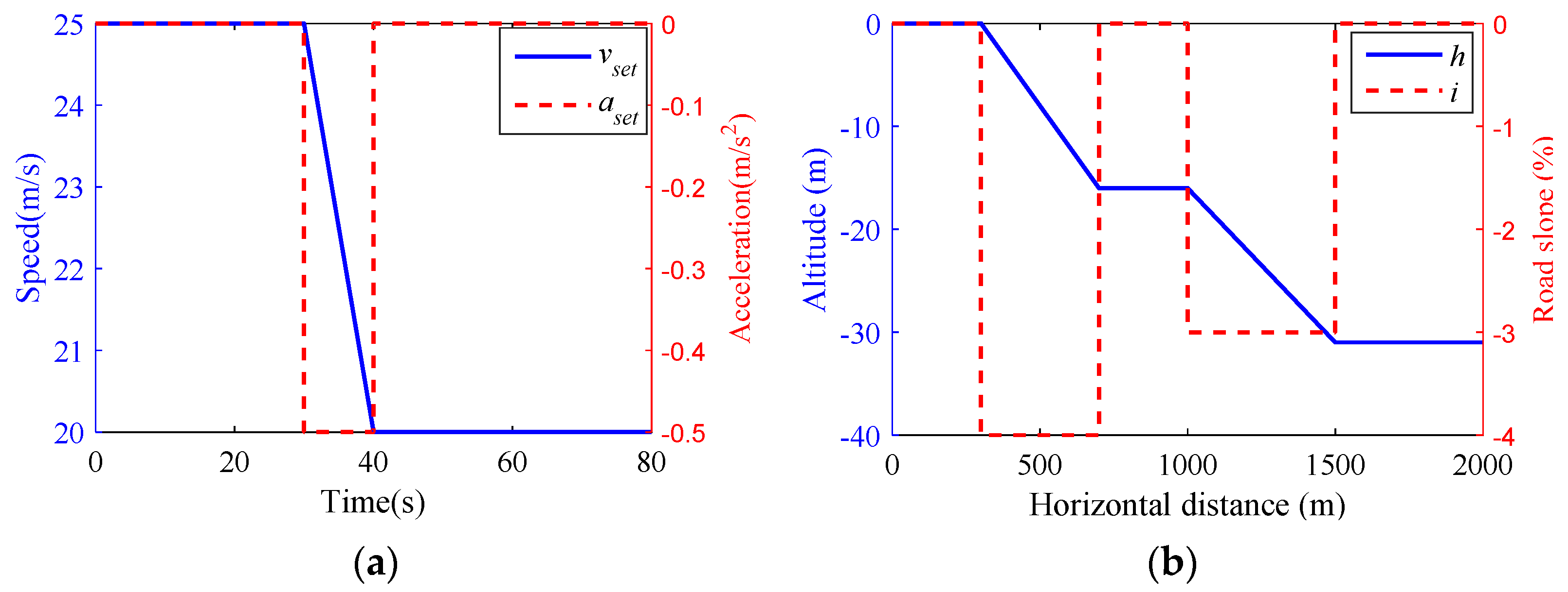
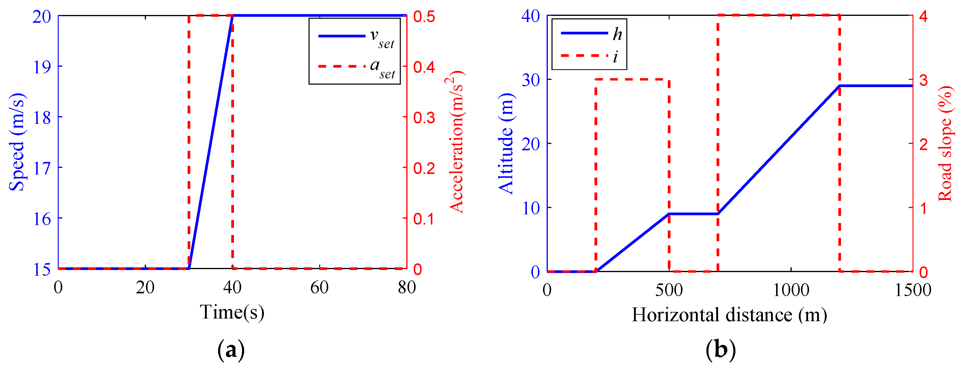
5.2. Experimental Setup and Parameter Settings

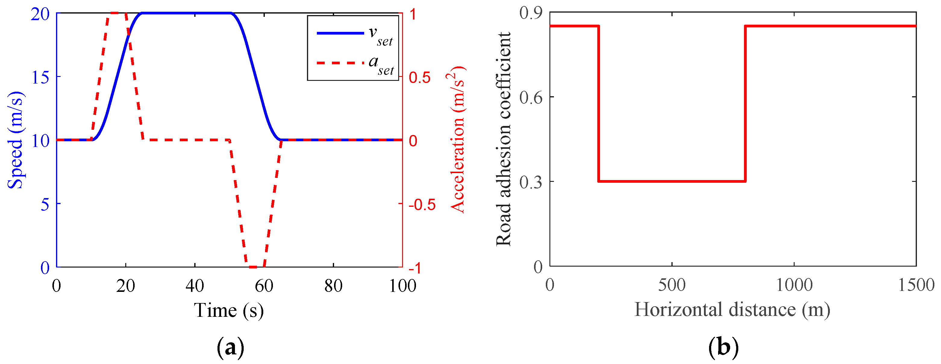
The proposed control method was compared with a conventional PID on the HIL platform under three scenarios. The parameters of the experimental conditions are shown in

Table 3. Experimental condition parameter settings.

Parameters	Scenario 1	Scenario 2	Scenario 3
Initial speed (m/s)	15	25	10
Road slope (%)	3 & 4	−3 & −4	0
Road adhesion coefficient	0.85	0.85	0.3 & 0.85
Desired time headway (s)	2	2	1.5
Maximum acceleration (m/s2)	0.5	−0.5	1

. The influence factors of the initial speed, road slope, road adhesion coefficient, time headway, and acceleration are considered. By setting the leading vehicle movement, the dynamic performance of the platoon at different speeds is tested. Among the three scenarios, the first involves the scenario where there are 3% and 4% uphill sections. The second scenario has −3% and −4% downhill sections. In addition, in order to test the effects of the platoon controller in rainy and snowy weather, the road adhesion coefficient is set to 0.85 and 0.3, respectively, in the third scenario.

• Scenario 1

The initial speed of the platoon is 15 m/s and the desired time headway is 2 s. After traveling at a constant speed for 30 s, the leading vehicle starts to accelerate at an acceleration of 0.5 m/s² for 10 s, and then the speed changes to 20 m/s. The first experimental scene of the leading vehicle movement and the road slope is shown in Figure 9.

• Scenario 2

The initial speed of the platoon is set to 25 m/s. When t = 30 s, the leading vehicle starts to decelerate to 20 m/s with a deceleration of 0.5 m/s². Then, the platoon keeps a time headway of 2 s and travels at a constant speed. Figure 10 shows the second experimental scene of the leading vehicle movement and the road slope.

• Scenario 3

At the initial moment, the platoon travels at a speed of 10 m/s for 10 s. Then, the leading vehicle generates an acceleration with the maximum value of 1 m/s², and the speed reaches 20 m/s. When t = 50 s, the leading vehicle generates a deceleration with the maximum value −1 m/s², and the speed returns to 10 m/s. The road adhesion coefficient is 0.3 for the section from 200 m to 800 m, and the remaining is 0.85. The third experimental scene of the leading vehicle movement and the road slope is shown in Figure 11.

In the simulations, the upper controller parameters based on conventional PID are adjusted manually. Through Equation (4), the controller parameters of the preceding vehicle and the host vehicle are different due to the different input. The lower controller has different values according to the driving and braking modes.

Table 4. The conventional PID controller parameters.

Parameters	Upper Controller		Lower Controller
	Preceding Vehicle	Host Vehicle	Driving Mode	Braking Mode
Kp	1	0.5	8000	5
Ki	0.5	0.5	3500	1
Kd	0.2	0.5	850	0.5

shows the values of conventional PID controller parameters. The control parameters are determined by the empirical knowledge from experts. The initial state of the platoon is set as the desired state, i.e., the initial distance errors and initial speed errors are all equal to 0.

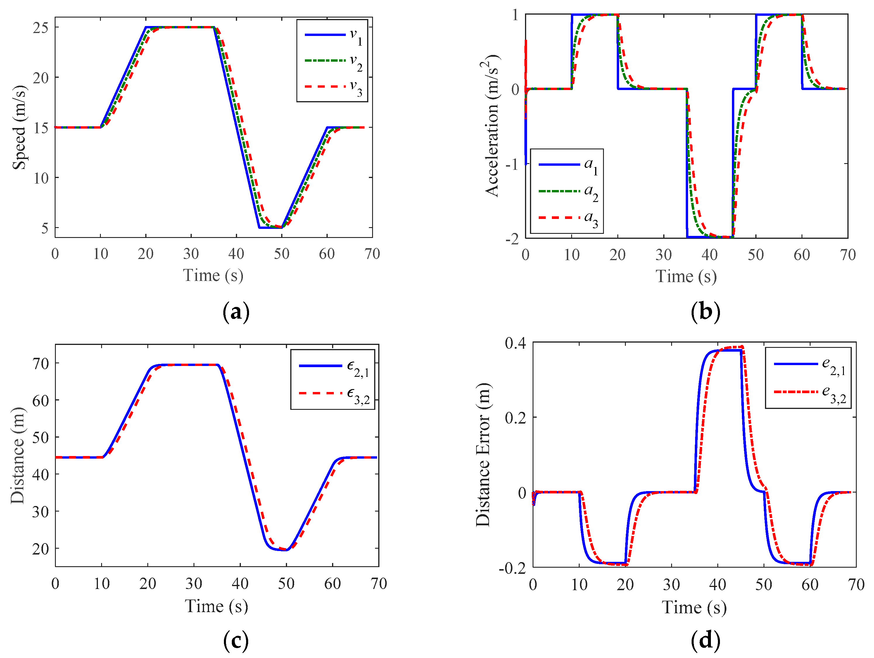
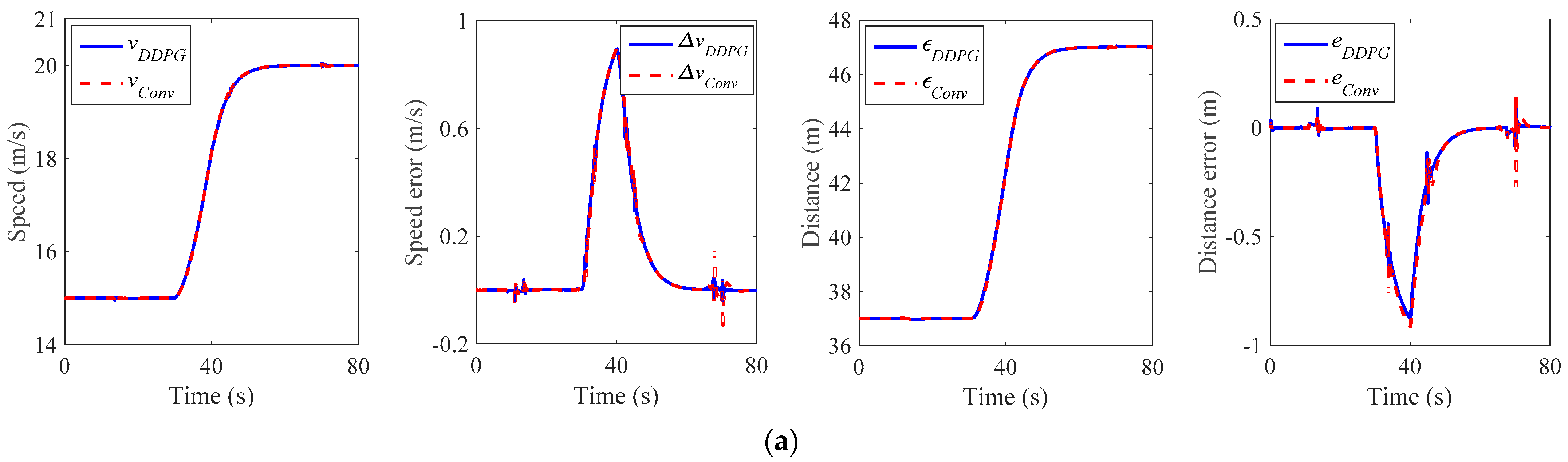
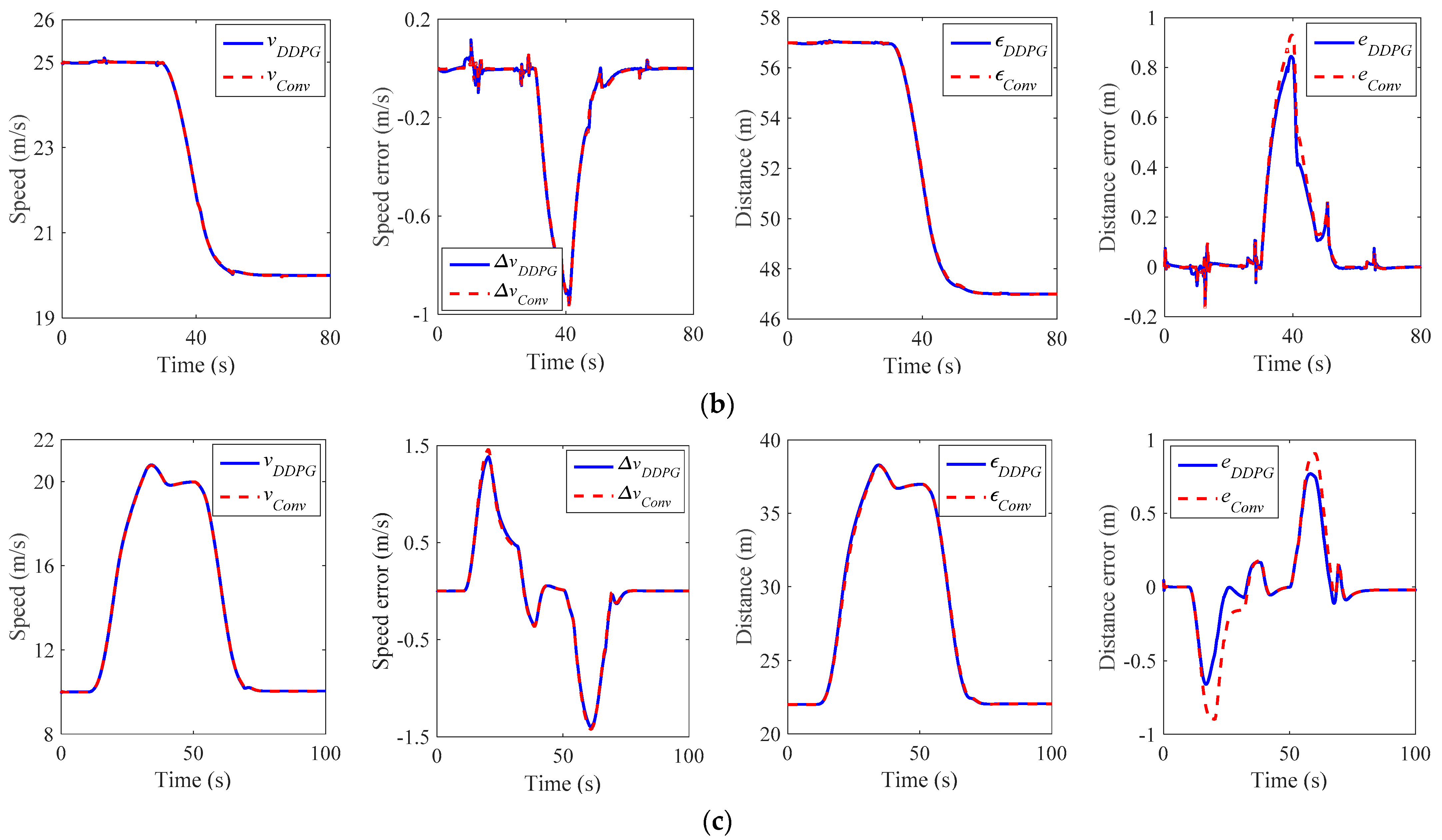
5.3. Validation Results

Scenario 1 is the experimental condition of the vehicle platoon accelerating uphill and Scenario 2 is the experimental condition of the vehicle platoon decelerating downhill. These two test scenarios verify the influence of the road slope, initial speed, and acceleration on the controller. The purpose of setting Scenario 3 is to test the influence of the road adhesion coefficient and time headway on the performance of the platoon controller. The speed, speed error, distance, and distance error performance of the host vehicle under three experimental conditions are shown in Figure 12.

As shown in Figure 12a, the maximum speed error and distance error of the host vehicle appear at the simulation time of 40 s. The maximum speed errors of DDPG-based and traditional PID are 0.88 m/s and 0.91 m/s. In addition, when the simulation time is 67–71 s, the curve vibrates rapidly due to the change of road slope. The speed error of the traditional control method is 0.15 m/s, while the speed error of DRL is less than 0.05 m/s, only 1/3 of the former. The maximum spacing errors of the DDPG-based and conventional PID are −0.87 m and −0.92 m, respectively. Similarly, the absolute value of the maximum distance error of the DDPG-based PID is 0.08 m in 67–71 s, while that of the conventional PID is 0.27 m.

From Figure 12b, the maximum speed errors of the DDPG-based and conventional PID are −0.95 m/s and −0.97 m/s. Compared with the uphill test scenario, the difference in distance error is more pronounced when driving on downward slopes. The maximum distance error of the DDPG-based controller is 0.85 m, while that of the conventional method is 0.93 m. In addition, due to the influence of road slope, the error curve fluctuates obviously in 8–14 s.

In the third experiment, there are obvious peaks and troughs in the curves of speed error and distance error where the road adhesion coefficient changes suddenly. In the third experiment, there are obvious peaks and troughs in the curves of velocity error and distance error where the road adhesion coefficient changes suddenly, as seen in Figure 12c. Due to the low adhesion coefficient of the road and the tire skids, the vehicle speed curve overshoots. The maximum speed error of the DDPG-based PID is 1.38 m/s, and the absolute value of the maximum distance error is 0.77 m. The maximum speed error and the absolute value of the maximum distance error of the conventional PID are 1.46 m/s and 0.90 m, respectively. Owing to its predefined PID control structure, the training process for the agent in the DRL-based PID control converges significantly faster than that in the DRL control [47]. The DRL-based PID control achieves a significant improvement over the traditional PID control by optimizing the controller parameters continuously [48,49]. It is strongly robust for system disturbances, which is better than that of a conventional PID controller [50].

6. Discussion

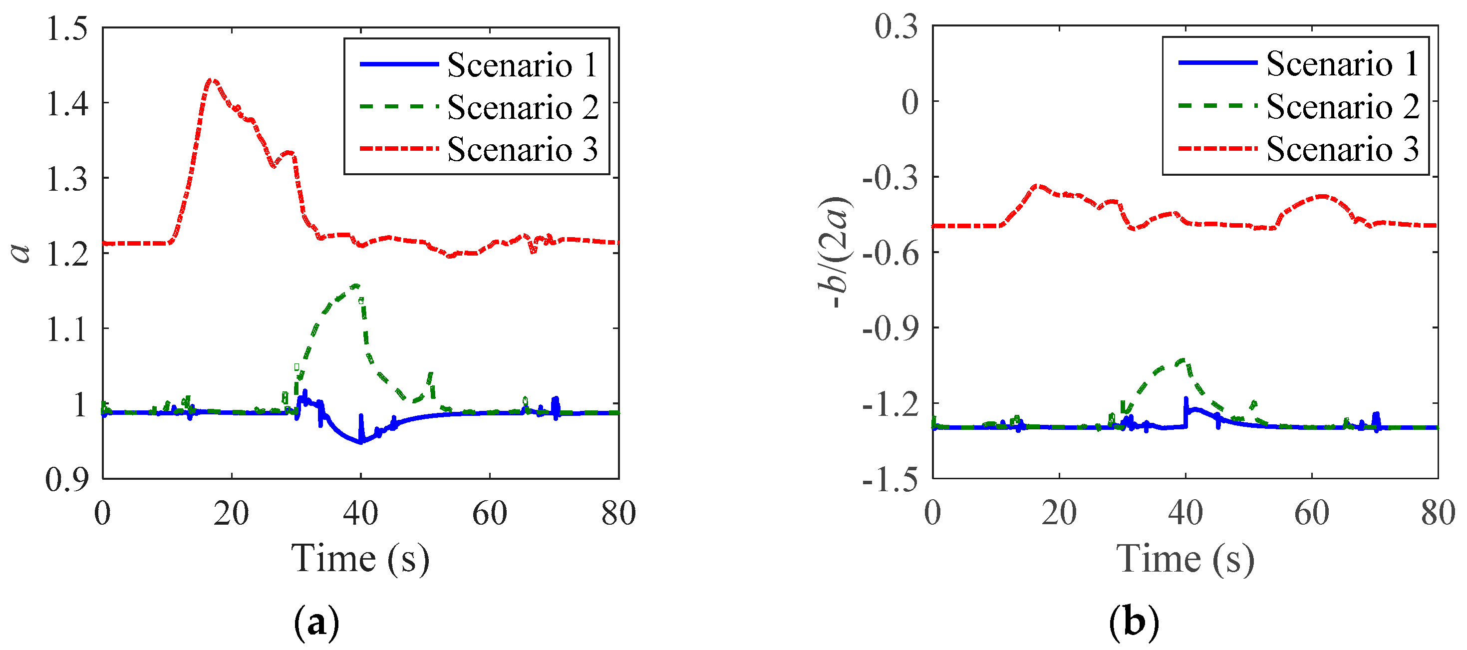
6.1. Stability Analysis

This section focuses on the stability analysis of homogeneous vehicular platoon control. The tendency of PID parameters (i.e., K_p, K_i, K_d) to change in the proposed method is shown in Figure 13. There are two kinds of stability for the platoon that need to be analyzed:

Internal stability. From the above experimental results, when the leading vehicle travels at a constant speed, the distance error between the host vehicle and the preceding vehicle gradually approaches 0, i.e.,$\underset{t\to \infty }{\lim }{e}_i\left(t\right)=0$, which means that internal stability can be guaranteed [40].

String stability. In the experiment, the values of parameters λ₁, λ₂, and τ are 0.5, 0.5, and 0.3 s, respectively. Based on (17), for the univariate function f (x) = ax² + bx + c, we can calculate the results of coefficients a and −b/2a, as shown in Figure 14.

It can be seen that in the whole simulation process a > 0, which means that the parabola opens upward. In addition, −b/2a < 0 means the axis of symmetry is located on the negative half of the coordinate axis. According to the parameter λ₁ = λ₂ = 0.5 and K_i > 0, the minimum value of quadratic function $f\left(0\right)=\left(1-{\lambda }_1\right)K_i^2>0$ always holds. Therefore, we will obtain |G(jω)|<1, which can satisfy the string stability condition of Equation (19) (see Section 2.3 Case A). In other words, the distance error of the vehicle platooning system is not amplified when transmitted to the following vehicles.

In summary, the vehicular platoon controller based on DDPG-based PID can meet the requirements of internal stability and string stability.

6.2. Control Effect Analysis

The performances of the two controllers are analyzed from the two indexes of the maximum speed error and the maximum distance error. The maximum speed error is the maximum value of the speed deviation between the host vehicle and the leading vehicle. The maximum distance error is the actual and desired distance maximum deviation between the host vehicle and the preceding vehicle. The comparison results are listed in

Table 5. Comparison of experimental results.

Scenario	Maximum Speed Error (m/s)		Improvement (%)	Maximum Distance Error (m)		Improvement (%)
	Conventional PID	DDPG-PID		Conventional PID	DDPG-PID
1	0.91	0.88	3.30	−0.92	−0.87	5.43
2	−0.97	−0.95	2.06	0.93	0.85	8.60
3	1.46	1.38	5.48	0.90	0.77	14.44

.

It is seen from Table 5 that the maximum speed error of the vehicular platoon based on the conventional PID controller is 1.46 m/s, while that of the DDPG-based PID controller is 1.38 m/s, which improves the performance by more than 5.48%. From the point of view of the maximum distance error, the DDPG-based PID controller is 0.13 m less than that of the conventional PID controller, and the maximum platoon stability time is reduced by 14.44%. In summary, comparing with the conventional PID, the DDPG-based PID not only has a better performance of tracking, but can also guarantee the string stability under different working conditions.

7. Conclusions

In this paper, we have proposed a DDPG-based PID learning control method, which uses a DDPG algorithm to automatically tune the PID weights for a vehicle platooning system. This method combines the offline learning ability of DRL with the advantages of the simple structure and easy implementation of a traditional controller PID, without relying on any manual tuning. Thus, the problem of insufficient adaptability of the traditional controller is solved. Moreover, compared with a single DRL algorithm, the proposed method has stronger interpretability and stability. The results of three experimental conditions show that the DDPG-based PID controller can meet the requirements of string stability under different road and vehicular platooning acceleration and deceleration conditions. In terms of the maximum speed error, the DDPG-based PID controller is 0.02–0.08 m/s less than the conventional PID controller, with a maximum reduction of 5.48%. In addition, the maximum distance error of the DDPG-based PID controller is 0.77 m, which is 14.44% less than that of the conventional PID controller. It can be seen from the above analysis that the DDPG-based PID controller has stronger robustness.

The future work would be focused on the optimization design of the neural network structure to improve the speed of convergence effectively and has better performance than the DRL algorithm. Besides, the HIL simulation simplifies the road environment conditions. The following research can carry out real vehicle experiments to further verify the stability and reliability of a vehicular platoon controller using DDPG-based PID.

References

1. Yang, J.; Peng, W.; Sun, C. A Learning Control Method of Automated Vehicle Platoon at Straight Path with DDPG-Based PID. Electronics 2021, 10, 2580. [Google Scholar] [CrossRef]
2. Talebpour, A.; Mahmassani, H.S. Influence of connected and autonomous vehicles on traffic flow stability and throughput. Transp. Res. Part C Emerg. Technol. 2016, 71, 143–163. [Google Scholar] [CrossRef]
3. Wang, Z.; Bian, Y.; Shladover, S.E.; Wu, G.; Li, S.E.; Barth, M.J. A Survey on Cooperative Longitudinal Motion Control of Multiple Connected and Automated Vehicles. IEEE Intell. Transp. Syst. Mag. 2020, 12, 4–24. [Google Scholar] [CrossRef]
4. Liu, B.; Gao, F.; He, Y.; Wang, C. Robust Control of Heterogeneous Vehicular Platoon with Non-Ideal Communication. Electronics 2019, 8, 207. [Google Scholar] [CrossRef] [Green Version]
5. Na, G.; Park, G.; Turri, V.; Johansson, K.H.; Shim, H.; Eun, Y. Disturbance observer approach for fuel-efficient heavy-duty vehicle platooning. Veh. Syst. Dyn. 2020, 58, 748–767. [Google Scholar] [CrossRef]
6. Chen, J.; Chen, H.; Gao, J.; Pattinson, J.-A.; Quaranta, R. A business model and cost analysis of automated platoon vehicles assisted by the Internet of things. Proc. Inst. Mech. Eng. Part D J. Automob. Eng. 2020, 235, 721–731. [Google Scholar] [CrossRef]
7. Hu, M.; Zhao, X.; Hui, F.; Tian, B.; Xu, Z.; Zhang, X. Modeling and Analysis on Minimum Safe Distance for Platooning Vehicles Based on Field Test of Communication Delay. J. Adv. Transp. 2021, 2021, 5543114. [Google Scholar] [CrossRef]
8. Wang, Z.; Wu, G.; Hao, P.; Boriboonsomsin, K.; Barth, M. Developing a platoon-wide Eco-Cooperative Adaptive Cruise Control (CACC) System. In Proceedings of the 2017 IEEE Intelligent Vehicles Symposium (IV), Los Angeles, CA, USA, 11–14 June 2017; pp. 1256–1261. [Google Scholar]
9. Karoui, O.; Guerfala, E.; Koubaa, A.; Khalgui, M.; Tovard, E.; Wu, N.; Al-Ahmari, A.; Li, Z. Performance evaluation of vehicular platoons using Webots. IET Intell. Transp. Syst. 2017, 11, 441–449. [Google Scholar] [CrossRef]
10. Fiengo, G.; Lui, D.G.; Petrillo, A.; Santini, S.; Tufo, M. Distributed Robust PID Control for Leader Tracking in Uncertain Connected Ground Vehicles with V2V Communication Delay. IEEE/ASME Trans. Mechatron. 2019, 24, 1153–1165. [Google Scholar] [CrossRef]
11. Rajaram, V.; Subramanian, S.C. Design and hardware-in-loop implementation of collision avoidance algorithms for heavy commercial road vehicles. Veh. Syst. Dyn. 2016, 54, 871–901. [Google Scholar] [CrossRef]
12. Guo, G.; Li, D. Adaptive Sliding Mode Control of Vehicular Platoons with Prescribed Tracking Performance. IEEE Trans. Veh. Technol. 2019, 68, 7511–7520. [Google Scholar] [CrossRef]
13. Huang, Z.; Chu, D.; Wu, C.; He, Y. Path Planning and Cooperative Control for Automated Vehicle Platoon Using Hybrid Automata. IEEE Trans. Intell. Transp. Syst. 2019, 20, 959–974. [Google Scholar] [CrossRef]
14. Liu, P.; Kurt, A.; Ozguner, U. Distributed Model Predictive Control for Cooperative and Flexible Vehicle Platooning. IEEE Trans. Control Syst. Technol. 2019, 27, 1115–1128. [Google Scholar] [CrossRef]
15. Yan, M.; Ma, W.; Zuo, L.; Yang, P. Distributed Model Predictive Control for Platooning of Heterogeneous Vehicles with Multiple Constraints and Communication Delays. J. Adv. Transp. 2020, 2020, 4657584. [Google Scholar] [CrossRef]
16. Li, S.E.; Gao, F.; Li, K.; Wang, L.; You, K.; Cao, D. Robust Longitudinal Control of Multi-Vehicle Systems—A Distributed H-Infinity Method. IEEE Trans. Intell. Transp. Syst. 2018, 19, 2779–2788. [Google Scholar] [CrossRef]
17. Zheng, Y.; Li, S.E.; Li, K.; Ren, W. Platooning of Connected Vehicles with Undirected Topologies: Robustness Analysis and Distributed H-infinity Controller Synthesis. IEEE Trans. Intell. Transp. Syst. 2018, 19, 1353–1364. [Google Scholar] [CrossRef] [Green Version]
18. Mnih, V.; Kavukcuoglu, K.; Silver, D.; Graves, A.; Antonoglou, I.; Wierstra, D.; Riedmiller, M. Playing atari with deep reinforcement learning. arXiv 2013, arXiv:1312.5602. [Google Scholar]
19. Lillicrap, T.P.; Hunt, J.J.; Pritzel, A.; Heess, N.; Erez, T.; Tassa, Y.; Silver, D.; Wierstra, D. Continuous control with deep reinforcement learning. arXiv 2015, arXiv:1509.0297. [Google Scholar]
20. Grigorescu, S.; Trasnea, B.; Cocias, T.; Macesanu, G. A survey of deep learning techniques for autonomous driving. J. Field Robot. 2020, 37, 362–386. [Google Scholar] [CrossRef]
21. Zhu, M.; Wang, X.; Wang, Y. Human-like autonomous car-following model with deep reinforcement learning. Transp. Res. Part C Emerg. Technol. 2018, 97, 348–368. [Google Scholar] [CrossRef] [Green Version]
22. Huang, Z.; Xu, X.; He, H.; Tan, J.; Sun, Z. Parameterized Batch Reinforcement Learning for Longitudinal Control of Autonomous Land Vehicles. IEEE Trans. Syst. Man Cybern. Syst. 2019, 49, 730–741. [Google Scholar] [CrossRef]
23. Wang, P.; Chan, C.; Fortelle, A.D.L. A Reinforcement Learning Based Approach for Automated Lane Change Maneuvers. In Proceedings of the 2018 IEEE Intelligent Vehicles Symposium (IV), Changshu, China, 26–30 June 2018; pp. 1379–1384. [Google Scholar]
24. An, H.; Jung, J.-I. Decision-making system for lane change using deep reinforcement learning in connected and automated driving. Electronics 2019, 8, 543. [Google Scholar] [CrossRef] [Green Version]
25. Chen, I.M.; Chan, C.-Y. Deep reinforcement learning based path tracking controller for autonomous vehicle. Proc. Inst. Mech. Eng. Part D J. Automob. Eng. 2020, 235, 541–551. [Google Scholar] [CrossRef]
26. Zhou, Y.; Fu, R.; Wang, C. Learning the Car-following Behavior of Drivers Using Maximum Entropy Deep Inverse Reinforcement Learning. J. Adv. Transp. 2020, 2020, 4752651. [Google Scholar] [CrossRef]
27. Makantasis, K.; Kontorinaki, M.; Nikolos, I. Deep reinforcement-learning-based driving policy for autonomous road vehicles. IET Intell. Transp. Syst. 2019, 14, 13–24. [Google Scholar] [CrossRef] [Green Version]
28. Ye, Y.; Zhang, X.; Sun, J. Automated vehicle’s behavior decision making using deep reinforcement learning and high-fidelity simulation environment. Transp. Res. Part C Emerg. Technol. 2019, 107, 155–170. [Google Scholar] [CrossRef] [Green Version]
29. Chen, B.; Wang, Y.; Lin, P. A Feedback Force Controller Fusing Traditional Control and Reinforcement Learning Strategies. In Proceedings of the 2019 IEEE/ASME International Conference on Advanced Intelligent Mechatronics (AIM), Hong Kong, China, 8–12 July 2019; pp. 259–265. [Google Scholar]
30. Wang, J.; Xu, X.; Liu, D.; Sun, Z.; Chen, Q. Self-Learning Cruise Control Using Kernel-Based Least Squares Policy Iteration. IEEE Trans. Control Syst. Technol. 2014, 22, 1078–1087. [Google Scholar] [CrossRef]
31. Dekker, L.G.; Marshall, J.A.; Larsson, J. Experiments in feedback linearized iterative learning-based path following for center-articulated industrial vehicles. J. Field Robot. 2019, 36, 955–972. [Google Scholar] [CrossRef]
32. Zhao, Q.; Xu, H.; Jagannathan, S. Neural Network-Based Finite-Horizon Optimal Control of Uncertain Affine Nonlinear Discrete-Time Systems. IEEE Trans. Neural Netw. Learn. Syst. 2015, 26, 486–499. [Google Scholar] [CrossRef]
33. Sahoo, A.; Xu, H.; Jagannathan, S. Neural Network-Based Event-Triggered State Feedback Control of Nonlinear Continuous-Time Systems. IEEE Trans. Neural Netw. Learn. Syst. 2016, 27, 497–509. [Google Scholar] [CrossRef]
34. Choi, S.; Kim, S.; Jin Kim, H. Inverse reinforcement learning control for trajectory tracking of a multirotor UAV. Int. J. Control Autom. Syst. 2017, 15, 1826–1834. [Google Scholar] [CrossRef]
35. Li, D.; Zhao, D.; Zhang, Q.; Chen, Y. Reinforcement Learning and Deep Learning Based Lateral Control for Autonomous Driving. IEEE Comput. Intell. Mag. 2019, 14, 83–98. [Google Scholar] [CrossRef]
36. Lu, C.; Gong, J.; Lv, C.; Chen, X.; Cao, D.; Chen, Y. A Personalized Behavior Learning System for Human-Like Longitudinal Speed Control of Autonomous Vehicles. Sensors 2019, 19, 3672. [Google Scholar] [CrossRef] [PubMed] [Green Version]
37. Xu, X.; Chen, H.; Lian, C.; Li, D. Learning-Based Predictive Control for Discrete-Time Nonlinear Systems with Stochastic Disturbances. IEEE Trans. Neural Netw. Learn. Syst. 2018, 29, 6202–6213. [Google Scholar] [CrossRef]
38. Ure, N.K.; Yavas, M.U.; Alizadeh, A.; Kurtulus, C. Enhancing Situational Awareness and Performance of Adaptive Cruise Control through Model Predictive Control and Deep Reinforcement Learning. In Proceedings of the 2019 IEEE Intelligent Vehicles Symposium (IV), Paris, France, 9–12 June 2019; pp. 626–631. [Google Scholar]
39. Yang, J.; Liu, X.; Liu, S.; Chu, D.; Lu, L.; Wu, C. Longitudinal Tracking Control of Vehicle Platooning Using DDPG-based PID. In Proceedings of the 2020 4th CAA International Conference on Vehicular Control and Intelligence (CVCI), Hangzhou, China, 18–20 December 2020; pp. 656–661. [Google Scholar]
40. Zheng, Y.; Li, S.E.; Wang, J.; Cao, D.; Li, K. Stability and Scalability of Homogeneous Vehicular Platoon: Study on the Influence of Information Flow Topologies. IEEE Trans. Intell. Transp. Syst. 2016, 17, 14–26. [Google Scholar] [CrossRef] [Green Version]
41. Swaroop, D.; Hedrick, J.K.; Chien, C.C.; Ioannou, P. A Comparision of Spacing and Headway Control Laws for Automatically Controlled Vehicles1. Veh. Syst. Dyn. 1994, 23, 597–625. [Google Scholar] [CrossRef]
42. Lu, X.; Shladover, S. Integrated ACC and CACC development for Heavy-Duty Truck partial automation. In Proceedings of the 2017 American Control Conference (ACC), Seattle, WA, USA, 24–26 May 2017; pp. 4938–4945. [Google Scholar]
43. Ploeg, J.; Shukla, D.P.; Wouw, N.V.D.; Nijmeijer, H. Controller Synthesis for String Stability of Vehicle Platoons. IEEE Trans. Intell. Transp. Syst. 2014, 15, 854–865. [Google Scholar] [CrossRef] [Green Version]
44. Zhu, M.; Chen, H.; Xiong, G. A model predictive speed tracking control approach for autonomous ground vehicles. Mech. Syst. Signal Process. 2017, 87, 138–152. [Google Scholar] [CrossRef]
45. Ntousakis, I.A.; Nikolos, I.K.; Papageorgiou, M. On Microscopic Modelling of Adaptive Cruise Control Systems. Transp. Res. Procedia 2015, 6, 111–127. [Google Scholar] [CrossRef] [Green Version]
46. Maas, A.L.; Hannun, A.Y.; Ng, A.Y. Rectifier nonlinearities improve neural network acoustic models. Proc. ICML 2013, 30, 3. [Google Scholar]
47. Wang, X.; Wang, R.; Jin, M.; Shu, G.; Tian, H.; Pan, J. Control of superheat of organic Rankine cycle under transient heat source based on deep reinforcement learning. Appl. Energy 2020, 278, 115637. [Google Scholar] [CrossRef]
48. Qin, Y.; Zhang, W.; Shi, J.; Liu, J. Improve PID controller through reinforcement learning. In Proceedings of the 2018 IEEE CSAA Guidance, Navigation and Control Conference (CGNCC), Xiamen, China, 10–12 August 2018; pp. 1–6. [Google Scholar]
49. Lee, D.; Lee, S.J.; Yim, S.C. Reinforcement learning-based adaptive PID controller for DPS. Ocean Eng. 2020, 216, 108053. [Google Scholar] [CrossRef]
50. Wang, X.-S.; Cheng, Y.-H.; Sun, W. A Proposal of Adaptive PID Controller Based on Reinforcement Learning. J. China Univ. Min. Technol. 2007, 17, 40–44. [Google Scholar] [CrossRef]
Figure 1. PLF topology structure diagram.
Electronics 10 02580 g001
Figure 2. Hierarchical control structure.
Electronics 10 02580 g002
Figure 3. Actor-critic neural network structures for DDPG.
Electronics 10 02580 g003
Figure 4. The framework of the training platform.
Electronics 10 02580 g004
Figure 5. Profile of leading vehicle movement state.
Electronics 10 02580 g005
Figure 6. Vehicle platoon tracking performance in training conditions. (a) Vehicle speed vi(t) (i = 1, 2, 3). (b) Vehicle acceleration ai(t) (i = 1, 2, 3). (c) Inter-vehicle distance between consecutive vehicles εi,i−1(t) (i = 2, 3). (d) The distance error with the desired distance ei,i−1(t) (i = 2, 3).
Electronics 10 02580 g006
Figure 7. Performance of total reward per episode and reward per step. (a) Total reward per episode. (b) Reward per step.
Electronics 10 02580 g007
Figure 8. Overall architecture of the HIL platform.
Electronics 10 02580 g008
Figure 9. Profiles of leading vehicle movement and road slope in scenario 1. (a) Leading vehicle movement. (b) Road slope.
Electronics 10 02580 g009
Figure 10. Profiles of leading vehicle movement and road slope in scenario 2. (a) Leading vehicle movement. (b) Road slope.
Electronics 10 02580 g010
Figure 11. Profiles of leading vehicle movement and road adhesion coefficient in Scenario 3. (a) Leading vehicle movement. (b) Road adhesion coefficient.
Electronics 10 02580 g011
Figure 12. Simulation results of host vehicle. (a) Scenario 1. (b) Scenario 2. (c) Scenario 3.
Electronics 10 02580 g012aElectronics 10 02580 g012b
Figure 13. Diagram of PID parameter changes under three experimental conditions. (a) Scenario 1. (b) Scenario 2. (c) Scenario 3.
Electronics 10 02580 g013
Figure 14. The parameter variation curve of the quadratic function. (a) Second-order coefficient a. (b) Axis of symmetry −b/2a.
Electronics 10 02580 g014