Android Malware Detection Based on Structural Features of the Function Call Graph

Abstract

The openness of Android operating system not only brings convenience to users, but also leads to the attack threat from a large number of malicious applications (apps). Thus malware detection has become the research focus in the field of mobile security. In order to solve the problem of more coarse-grained feature selection and larger feature loss of graph structure existing in the current detection methods, we put forward a method named DGCNDroid for Android malware detection, which is based on the deep graph convolutional network. Our method starts by generating a function call graph for the decompiled Android application. Then the function call subgraph containing the sensitive application programming interface (API) is extracted. Finally, the function call subgraphs with structural features are trained as the input of the deep graph convolutional network. Thus the detection and classification of malicious apps can be realized. Through experimentation on a dataset containing 11,120 Android apps, the method proposed in this paper can achieve detection accuracy of 98.2%, which is higher than other existing detection methods.

1. Introduction

The Android operating system is widely used in smart mobile terminals such as smartphones, tablets, and wearable devices. Statistics from International Data Corporation (IDC) [1] show that Android occupies more than 85% of the global market of mobile operating systems, which is more than five times the share of the second largest system, iOS. As of May 2019, Android possesses more than 2.5 billion monthly active users [2], ranking first among all operating systems including desktop operating systems. Android has become very popular due to it being open source and free, but this has also made Android a main target for malware attacks. An assessment report jointly issued by Kaspersky Lab and INTERPOL [3] shows that more than 98% of mobile phone malware targets Android devices. Another report [4] pointed out that about 5000 new mobile phone malicious program samples were intercepted on an average day in 2019.

The traditional detection method based on signature is utilized by security protection software, which detects malicious apps by extracting the signature from the application installation package and comparing it with the signature in the known malware database. However, signature-based detection method is unable to detect unknown apps outside the database. At the same time, the number of Android malicious apps has surged. It takes a lot of time and resources to detect massive malicious samples using manual methods. All the above situations have brought great pressure on Android malware detection. In order to meet the above challenges, Android malware detection based on machine learning have been widely used and achieved good detection results, becoming a more effective choice against emerging malicious apps.

Android malware detection based on machine learning usually includes two main steps: feature construction and classification. The first step is to extract the features of the application sample set through static analysis or dynamic analysis. Static analysis is mainly to analyze the application installation package to obtain the set of permissions, components, operation code sequence and so on; the dynamic analysis is to analyze the state of the application at runtime to obtain the API call sequence, stack usage or other features. The second step is to use a suitable machine learning algorithm to train the feature representation obtained in the first step, and the trained model can be generated to predict the category of unknown apps.

In the feature construction step, previous research work has proposed many effective feature representations. Researches [5,6,7,8,9] take the permission mechanism of Android as the research object, mining the frequent item sets of permissions requested by the application for machine learning training, and achieved a good classification detection effect. Android apps interact with devices through API calls, and similar apps generally have similar API call patterns. Therefore, researches [10,11,12] extract the set of API calls in the application source code as features to detect malware. Compared with the simple combination of permissions or API features, Pei et al. [13] utilize natural language processing to convert the combination of permissions and API calls into a graph before further processing. Although this method achieved better results than previous approaches, the call relationship between APIs is not considered in the graph modeling, and it cannot reflect the potential behavior of the application. The above approaches have achieved high detection accuracy in classifying Android benign apps and malicious apps, but using this coarse-grained information to describe the behavior of apps is not accurate and complete, because the permissions or APIs used by benign apps and malicious apps may overlap, they cannot be well distinguished. Therefore, the work of Fan et al. [14] and Ge et al. [15] focus on the behavior patterns of apps, taking the function call graph of the application as the research object, and measuring the similarity between apps by calculating the similarity of the graph; so as to realize the classification and detection of malicious apps. Since the function call graph is a visualization of the internal functions of the application and represents the potential behavior of the application, on the one hand, it can obtain a more fine-grained feature representation than the permissions or API combinations; on the other hand, malicious apps can be prevented, to a certain extent, from using obfuscation means of changing function names to avoid detection, because no matter how the function is renamed, the topological relationship contained in the function call graph will not be changed. Therefore, this paper adopts a function call graph with node structure attributes as the feature of application detection.

In the classification step, for the training of graph features, most of the previous researches are to embed the node features of the graph into the vector space, and then use convolutional neural networks (CNN) for training, and further realize the malware detection. However, because the spatial features of graph data have two attributes, node features and structural features, the previous methods [14,15] only consider node features and ignore structural features, reducing the dimensionality of structured graph data to vector space, which lose the topological information when the structural graph data is reduced to vector space. The topological structure contained in the function call graph is an effective representation of different application features, which can distinguish malicious apps from benign apps. Therefore, taking structural features into account can achieve better detection results. In recent years, with the emergence of large-scale graph data such as social networks and recommendation systems, graph convolutional networks have begun to appear in people’s visions. Because graph convolutional networks can automatically learn the association information between nodes and extract the structural features of graphs, it has been widely used in chemical molecular structure classification, citation network node classification and social network division. In this paper, considering the structural features of the function call graph, the graph convolutional network is applied to Android malware detection, and a deep graph convolutional network framework that directly conducts end-to-end learning of graph features is designed to achieve detection.

The main contributions of this paper are summarized as follows:

(1)

We propose a feature representation of the function call graph with node structure attributes, which not only expresses the calling relationship between functions, but also contains the topology information between multi-hop function nodes;

(2)

We implement a DGCNDroid framework that uses the deep graph convolutional network for Android malware detection. The framework directly uses the function call graph as the input of the depth graph convolutional network to convert the malicious application detection problem into a graph classification problem without compressing the graph data into low-dimensional vectors, retaining more complete graph structure information;

(3)

Compared with the existing methods that use features of permission combination, API combination and graph embedding, the method proposed in this paper has higher detection accuracy rate and lower false positive rate.

The remainder of this paper is organized as follows. Section 2 reviews the related work on Android malware detection based on machine learning and the development of graph convolutional networks. Section 3 elaborates the proposed DGCNDroid framework. Section 4 discusses results and evaluations of experiment. Finally, Section 5 concludes the paper.

2. Related Work

2.1. Android Malware Detection Based on Machine Learning

According to the method of obtaining features, Android malware detection can be divided into methods based on static analysis, methods based on dynamic analysis and methods based on hybrid analysis.

Static analysis mainly analyzes and extracts features for the decompiled code and configuration files of the Android .apk file, without actually executing the application. Arp et al. [16] proposed a lightweight method for detecting Android malicious apps—Drebin. This method extracted eight static features such as permissions and components from the decompiled code and manifest files of the application. Then the support vector machine (SVM) was used to train the samples and achieved a detection rate of 94% in the case of low false alarms. Zhu et al. [17] proposed DeepFlow, which is a detection method based on the features of static data flow inside Android apps. It utilized deep brief network (DBN) to establish a classification model and achieved an F1 score of 95.05%. Li et al. [18] used deep neural network (DNN) to detect malicious apps based on the combination of permissions and API features. This method can detect 97% of malicious software with a false positive rate of 0.1%. Xu et al. [19] used long short-term memory (LSTM) training model on the semantic features of Android bytecode, and the accuracy of detecting malware can reach 97.74%. Literature [20] used Hamming distance to measure the similarity of application samples and proposed four malware detection methods based on improved K-nearest neighbor (KNN). Permission, API and intention features were verified experimentally on three different data sets. The results show that the accuracy of the proposed algorithm is more than 90%, and the detection accuracy is up to 99% under the API features.

Dynamic analysis monitors and discovers malicious behavior of the application by running the application on a real machine or simulator. Liang et al. [21] regarded the system call sequence as text processing, then used CNN to train this feature and achieved a detection accuracy of 93.16%. Ref. [22] proposed a detection framework called “Andromaly” to monitor events such as the number of data packets sent by mobile devices through the network, the number of running processes and battery power, then multiple classifiers were used to classify the original dataset in different scenarios. Hou et al. [23] proposed an Android malware detection system called “Deep4MalDroid”, which used the Linux kernel system call graph as a feature. Finally, it used the stacked auto-encoder (SAE) as a classifier and achieved 93.68% classification accuracy on a dataset that contained 3000 applications. Ananya et al. [24] proposed Sysdroid, a dynamic analysis method based on system calls, and a new feature selection method to improve the performance of the classifier. Experiment results on different classifiers showed that the accuracy is between 95% and 99%.

Hybrid analysis combines dynamic analysis with static analysis to obtain more comprehensive features. The authors in Ref. [25] firstly used dynamic analysis to extract features such as system calls, network traffic and request permissions during application running, and then used static analysis to extract features of application components, and finally conducted classification detection through DNN with 95% accuracy. The Droid-Sec method proposed by Yuan et al. [26] used static analysis and dynamic analysis to extract more than 200 features for malicious application detection. Compared with traditional machine learning methods such as decision tree and multi-layer perceptron, it shows that the detection effect of the deep learning method is better, and it can achieve 96% accuracy in a real Android application dataset. The authors in Ref. [27] proposed MADAM and analyzed correlated features at four levels: kernel, application, user and package to detect malicious behaviors, which made comprehensive use of both static and dynamic features such as application metadata, API calls, user behavior, services short message service (SMS) and system calls.

Compared with the methods that often use permissions, API or intention as features in static analysis, the advantage of the proposed approach is that it uses the function call graph for features. The features expressed in this paper have function call information and can better describe the behavior of the application, while the combination of permissions, API or intention cannot reflect the relationship between the feature elements. Compared with other works using graph as the research object, we consider the structural feature of the function call graph, and use a graph convolution network to further extract the feature. However, previous work transformed the function call graph into a vector, which lost the structural information of the function call graph.

Compared with dynamic analysis and hybrid analysis, the advantages of our method are mainly reflected in the advantages of static analysis compared with dynamic analysis. Static analysis has the characteristics of fast execution speed and high code coverage, while dynamic analysis has high resource overhead and it is difficult to trigger all malicious behaviors. Although static analysis is easily affected by code confusion, considering the structure features in our approach, we can avoid the impact of function renaming to a certain extent, because renaming will not change the topology of function call graphs.

2.2. Graph Convolutional Network

In recent years, machine learning has been widely used in various tasks such as speech recognition, image classification and natural language processing. The data objects processed in these tasks are usually represented as well-structured Euclidean space data. For example, images can be represented as regularly arranged pixels in Euclidean pace. Therefore, CNN can use the globally shared convolution kernel to learn the hidden layer representation information. However, as non-Euclidean data such as relational networks and knowledge graphs are increasingly being explored as research objects, the irregularities of graph data pose challenges to existing machine learning algorithms. Unlike images, which can be represented as a regular grid in Euclidean space, the graph is composed of a series of nodes (objects) and edges (relationships), which express the interdependence between objects, and the number of its neighbors is not fixed. The structure difference between the image and the graph is shown in Figure 1. Figure 1a is an image of the number “9” in the handwritten digit database from Modified National Institute of Standards and Technology (MNIST), which is composed of a 28 × 28 regular pixel grid. It can be expressed as a matrix; Figure 1b is a graph composed of nodes and edges. The arrangement of the nodes is irregular, and the number of neighbor nodes of the node is not fixed. The traditional convolution operation used for image processing cannot be directly applied to graph data. It is necessary to find a learnable convolution kernel suitable for graphs. So recently there has been research on extending the application of CNN to graph data, which is called the graph convolutional network (GCN).

Figure 1. (a) An image of the number “9” in the MNIST handwritten digit database and (b) a graph composed of nodes and edges.

Graph convolutional networks are mainly divided into two research directions, spectral convolution and spatial convolution.

The method based on spectral convolution defines the graph convolution in the spectral domain by calculating the eigenvector of the graph Laplacian matrix. Bruna et al. [28] first proposed a graph convolution network based on spectrum, but the algorithm is more complex for large graph data, so Defferrard et al. [29] used Chebyshev polynomials to fit the convolution kernel, and the spectrum filter was parameterized by Chebyshev polynomials of eigenvalues to reduce computational complexity. Kpif et al. [30] introduced the first-order approximation ChebNet to improve previous work. This method greatly improved the computational complexity of the previous method and has become the most widely used method of graph convolution in spectral domain. The above-mentioned methods based on the frequency domain have a common feature that the graph Laplacian matrix used is a symmetric matrix, so this type of method is not suitable for the processing of directed graph data.

The method based on spectral convolution defines the graph convolution by the connection relationship of each node, and the graph convolution is defined by obtaining information from the node itself and its neighboring nodes, which is closer to the convolution operation in the traditional CNN. Based on the idea of graph kernel, Zhang et al. [31] proposed a deep graph convolutional network that extracts multi-scale nodes’ features, and achieved good results in graph classification. The GraphSage method proposed by Hamilton et al. [32] trained a set of aggregation functions to sample and aggregate feature information such as different hops or search depths from the neighborhood of the current node, without the need to perform convolution operations on the entire graph. Niepert et al. [33] proposed a PATCHY-SAN framework that can convolve any kind of graphs, by converting the graph structure into a sequence structure, then they used CNN to perform convolution on the transformed sequence structure.

In summary, the method based on spectral domain is suitable for undirected graphs, while the method based on spatial domain can be used for both undirected graphs and directed graphs. Since the feature of the API call graph extracted in this paper is a directed graph, in order to better retain the directed information of the call relationship, we choose a graph convolution method based on spatial domain to train this feature.

3. Android Malware Detection Based on Structural Features of Function Call Graph

In this paper, a graph convolutional network is applied to Android malicious application detection, and the detection framework DGCNDroid is designed. Its overall architecture is shown in Figure 2. It is mainly composed of three stages: the first is the feature construction stage, where sensitive API call graphs containing structural information were extracted from the application training set; the next stage is deep learning by the graph convolution network, where the features extracted in the first stage are sent to the deep graph convolution network for training, and the classification model is generated; and the last is the detection stage, where the classification model generated in the second stage is used to classify the apps without labels in the test set, and the classification effect of the model will be evaluated.

Figure 2. The overall architecture of DGCNDroid.

3.1. Constructing Features from Function Call Graphs

3.1.1. Extracting Function Call Graphs

Android apps are usually written in Java, compiled and stored in the classes.dex file which is executable by the Dalvik virtual machine, and packaged as the .apk file together with the required resources and manifest files. This paper utilizes the reverse analysis tool Androguard to extract the function call graph of apps.

Definition 1.

Function call graph of an Android application is a directed graph, represented by$G=(V,E)$and composed of a node set V and an edge set E.$V=\left\{v_i|i=1,2,\dots ,n\right\}$represents the function set used by the application, and each$v_i\in V$represents a function name.$E=\{⟨v_i, v_j⟩{|v}_i{,v}_j\in V\}$represents the set of call relationships between functions, and the ordered pair$⟨v_i, v_j⟩$represents the call of function$v_i$to$v_j$. Figure 3 shows part of the function call graph of a malicious application of the family DroidKungfu in the dataset Drebin [16].

Figure 3. Part of the function call graph of the malware in DroidKungfu (SHA1: a6f39574437c2de53ea881d589408753f2539e3c).

3.1.2. Generating Subgraphs with Sensitive APIs

The Android platform provides thousands of APIs. Analysis of all function calls not only consumes a lot of computing resources, but also fails to highlight the differences between different types of apps. Therefore, in the work of this paper, we focus on sensitive APIs controlled by Android permissions [34]. Android apps can access sensitive resources and perform sensitive operations through sensitive APIs. We select APIs in 11 sensitive packages that are often used by malicious applications. These 11 packages cover the most sensitive resources of the Android system, such as messages, calls, location and network information, as shown in Table 1.

Definition 2.

Subgraph of sensitive API calls is represented by$SG=(V^{\prime },E^{\prime })$and composed of the set$V^{\prime }$, which contains sensitive API call nodes and their neighbors, and the set$E^{\prime }$, which contains edges formed by these nodes. It is an induced subgraph of the original function call graph. The set of nodes of sensitive API is denoted as$V_s$, then$V^{\prime }=\left\{v_j\right|\exists v_i\in V_s\cup V,\mathit{distance}\mathit{(}{v}_i,v_j\mathit{)}=0,1,v_j\in V^{\prime }\}\mathit{,} E^{\prime }=\{⟨v_i,v_j⟩|v_i\mathit{,} v_j\in V^{\prime }\}$, where distance() is the function to calculate the shortest distance between two nodes.

Table 1. 11 Android sensitive class packages.

	Class Name	Sensitive Information/Operation Included
1	android.accounts	User’s online account information
2	android.app	Application management
3	android.bluetooth	Bluetooth management
4	android.content	Content sharing
5	android.location	Geographical location information
6	android.media	Multimedia management
7	android.net	Networking
8	android.nfc	Near Field Communication (NFC)
9	android.provider	Storage accessing
10	android.telecom	Calling management
11	android.telephony	Message and device information

The pseudo code of the algorithm for generating the subgraph of sensitive API calls from the original function call graph is shown in Algorithm 1.

Algorithm 1 Generating the subgraph of sensitive API calls

Time complexity of generating the subgraph of sensitive API calls algorithm is detailed as follows:

Algorithm 1 is divided into two successive processes. First, it finds whether the sensitive API nodes are included in the original graph, and then it finds the edges containing sensitive nodes in the original graph. Suppose that the number of nodes in the original function call graph $G$ is n, and the number of nodes in the sensitive API nodes set $V_s$ is m. Every time one node is taken out from $V_s$ and matched with all the nodes in $G$, it is recorded as the node of subgraph SG. Each m node needs to be matched n times, so the time complexity of the process of finding sensitive nodes is O (n × m). At the same time, the edge of the sensitive function call subgraph is found. Suppose the number of sensitive nodes found is k, and each sensitive node needs to be combined with the nodes in the original graph $G$ to determine whether the edge exists, then the time complexity of this process is O (n × k). Therefore, the total time complexity should be O (n × m) + O (n × k) = O (n × m).

3.1.3. Obtaining the Structural Features of the Sensitive API Call Subgraph

The structural features of the sensitive API call subgraph include two elements, the adjacency matrix and the structural attributes of the nodes.

Definition 3.

Adjacency matrix of the graph$G=(V,E)$is a square matrix with the following properties.

$${\mathit{A}}_{ij}=\{\begin{array}{c}1,<v_i,v_j>\in E(G)\\ 0,<v_i,v_j>\in E(G)\end{array}$$

(1)

Although a large number of custom functions and third-party API nodes in the original function call graph were deleted in the stage of generating the sensitive API call subgraph, we calculated the two types of structural attribute features of the nodes in the sensitive API subgraph, namely the centrality measure of nodes in the original function call graph and the vector of the number of neighboring nodes within n-hops.

The centrality measure used in this paper includes the following two kinds:

(1) Betweenness centrality

The betweenness centrality of a node in the graph refers to the ratio of the number of shortest paths passing through the node between two nodes in the graph to the number of all the shortest paths between these two nodes, which indicates the degree of interaction between a node and other nodes. In a graph, the node with higher betweenness centrality has stronger control ability, because more information will be passed through the node. The betweenness centrality $B{(v}_i)$ of node $v_i$ can be calculated by Equation (2), where ${\sigma }_{v_s{v}_t}$ is the sum of all shortest paths from source node $v_s$ to destination node $v_t$, and ${\sigma }_{v_s{v}_t}{(v}_i)$ represents the number of times that the shortest path passes through $v_i$.

$$B(v_i)={\displaystyle \sum _{v_s\ne v_i\ne v_t}\frac{{\sigma }_{v_s{v}_t}(v_i)}{{\sigma }_{v_s{v}_t}}}$$

(2)

(2) Closeness centrality

The closeness centrality of a node in the graph refers to the reciprocal of the average distance between the node and other nodes. This indicator can be used to measure the length of time that information is transmitted from the node to other nodes. The closeness centrality ${C(v}_i)$ of node $v_i$ can be calculated from Equation (3), where N is the number of all nodes, and distance ($v_i$ $v_j$) represents the distance between $v_i$ and $v_j$.

$$C(v_i)=\frac{N-1}{{\displaystyle \sum _{j\ne i}distance(v_i,v_j)}}$$

(3)

Definition 4.

N–hop neighboring nodes. If the shortest path between node$v_i$and node$v_j$in the graph needs to pass through$n$edges, then node$v_j$is the n-hop neighboring node of node$v_i$. When n-hop neighboring nodes are found, the edge of the function call graph is regarded as undirected edge. As shown in Figure 4, for node$v_1$, there are four 1-hop neighboring nodes as shown in yellow and two 2-hop neighboring nodes as shown in blue. It is worth noting that although there are two paths from$v_1$to$v_2$in the graph, we consider the shortest path and$v_2$should be regarded as the 1-hop neighboring node of$v_1$.

Figure 4. n-hop neighboring nodes of node v1.

The pseudo code of algorithm for calculating the vector of the number of neighboring nodes within n hops is shown in Algorithm 2.

Algorithm 2 Calculating the vector of the number of neighboring nodes within n hops

Finally, after the above calculation, each node $v_i$ has a structural feature vector of the following form:

$$\mathit{x}\left(v_i\right)=\left(B\left(v_i\right),C\left(v_i\right),\mathit{N}\left(1\dots n\right)\right)$$

(4)

3.2. Design of Deep Graph Convolutional Networks

The overall design of deep graph convolutional networks used in this paper is shown in Figure 5. The processing of the input graph data consists of three stages:

Figure 5. Overview of the model of deep graph convolutional network.

(1)

Multi-layer graph convolution layers cascade to extract the structural features of nodes of different depths;

(2)

The global pooling layer sorts the nodes according to the PageRank score of the nodes, and unifies the output size of each graph convolution layer;

(3)

The traditional convolution layer further extracts the features represented by the graph convolution, and the fully connected layer performs classification prediction.

3.2.1. Graph Convolutional Layer

Given the graph $G$, A is the adjacent matrix of G, and n is the number of all nodes in G. Each node has a c–dimension structural feature vector x, and the structural feature vectors of all nodes constitute the feature matrix X.

As shown in Figure 6, the aggregation features of node $v_i$ can be obtained by the weighted average of the structural features of their neighboring nodes, which can be written as the matrix form:

$$\mathit{H}=\mathit{f}({\widehat{\mathit{D}}}^{-1}\widehat{\mathit{A}}\mathit{X}\mathit{W})$$

(5)

where $\widehat{\mathit{A}}=\mathit{A}+\mathit{I}$ and $\mathit{I}$ is the identity matrix. The function of $\widehat{\mathit{A}}$ is to add features of node $v_i$ itself by adding self-loops. $\widehat{\mathit{A}}$ is the degree matrix corresponding to $\widehat{\mathit{A}}$, and the matrix element is ${\widehat{\mathit{D}}}_{\mathit{i}\mathit{i}}={\displaystyle {\sum }_{\mathit{j}}{\widehat{\mathit{A}}}_{\mathit{i}\mathit{j}}}$. $\mathit{W}$ is the parameter matrix that the neural network needs to train. f is the nonlinear activation function. $\mathit{H}$ is the output matrix of the convolutional layer.

Figure 6. The aggregation of node structural features.

By iterating Equation (5), the output of multiple graph convolutional layers in Equation (6) can be obtained.

$${\mathit{H}}^{\mathit{l}+1}=\mathit{f}({\widehat{\mathit{D}}}^{-1}\widehat{\mathit{A}}{\mathit{H}}^{\mathit{l}}{\mathit{W}}^{\mathit{l}})$$

(6)

3.2.2. Global Pooling Layer

The main role of the global pooling layer is to sort the feature descriptions extracted from the convolutional layer of the graph according to the importance of nodes, and then cut them to a uniform size for input into the traditional convolutional layer and the fully connected layer.

A basic assumption is that more important functions tend to be called by other functions more. In the initial stage, each function node is given the same PageRank score, and then according to the calling relationship between functions, the PageRank score of the current node is updated by all the nodes that call it for multiple rounds until convergence. In each round of PageRank score update, the calling node distributes its current PageRank score to the edges on average, and the called node can update the current PageRank score by summating all the scores passed by the edge pointing to this node. The PageRank score of a node $v_i$ can be calculated by the following Equation (7), where $v_j$ is the function node calling $v_i$ and PR($v_j$) is the PageRank score of node $v_j$. L($v_j$) is the number of nodes $v_j$ points to other nodes, d is the correction coefficient, N is the number of all nodes:

$$PR(v_i)=\frac{1-d}{N}+d{\displaystyle \sum _{v_j}\frac{PR(v_j)}{L(v_j)}}$$

(7)

As shown in Figure 5, the output of the l-th graph convolution layer is ${\mathit{H}}^l,l=1,2,\dots ,m$, and the input of the global pooling layer is the output cascade ${[\mathit{H}}^1{,\mathit{H}}^2{,\dots ,\mathit{H}}^{\mathrm{m}}]$ of each graph convolution layer. The output of the graph convolution layer is a n-dimension tensor, where each dimension is the feature description of a node. By calculating the PageRank score of each node, the output tensor is sorted according to the descending order of the score value. The output of the global pooling layer intercepts the first output tensor in the way of top-k, which is usually taken as the number of nodes that more than 60% of graphs have. In this paper, the value of k is 80. Finally, the output tensor size is unified by deleting the last n – k lines or adding k – n zero lines when k > n.

3.2.3. Traditional Convolution Layer and Full Connection Layer

The traditional convolution layer and fully connected layer follow the global pooling layer, including two one-dimensional convolution layers, one max pooling layer and one fully connected layer. The first one-dimensional convolution layer has 16 output channels, and the kernel size and stride are set to the number of nodes in the graph convolution layer. The next is a maximum pooling layer, whose sampling kernel size is 2 and stride is 2. The second one-dimensional convolution layer with a sampling kernel size of 5 and stride of 1 has 32 output channels. Then there is a fully connected layer with 128 hidden layer nodes. Finally, the softmax function outputs the classification results.

4. The Experimental Evaluation

4.1. Experimental Platform and Dataset

In this paper, the experimental platform is equipped with an Intel(R) Core(TM) I7-8750h@2.2 gHz CPU, NVIDIA GeForce GTX 1070 GPU and 32 GB memory. The operating system is 64-bit Windows 10, and the machine learning platform is TensorFlow 2.1.0. The code is all implemented in Python.

The experimental dataset used in this paper contains a total of 11,120 Android applications, including 5560 malicious application samples from the dataset Drebin [16] and 5560 benign application samples collected from 360 Mobile Assistant (http://zhushou.360.cn/). Malicious application samples are classified according to the family, and the specific number of malicious application samples of top-20 families is shown in Table 2.

Table 2. Sample distribution of top-20 families of malicious apps.

Id	Malware Family	Number	Id	Malware Family	Number
1	FakeInstaller	925	11	ADRD	91
2	DroidKungFu	667	12	DroidDream	81
3	Plankton	625	13	LinuxLotoor	70
4	Opfake	613	14	GoldDream	69
5	GingerMaster	339	15	MobileTx	69
6	BaseBridge	330	16	FakeRun	61
7	Iconosys	152	17	SendPay	59
8	Kmin	147	18	Gappusin	58
9	FakeDoc	132	19	Imlog	43
10	Geinimi	92	20	SMSreg	41

4.2. Metrics

In this paper, the confusion matrix is used as the basis metrics of the machine learning model. The rows of the confusion matrix represent the predicted categories of machine learning, and the columns represent the actual categories of the samples. As shown in Table 3, true positive (TP) means that the predicted category is malicious application and the actual category is also malicious application; false positive (FP) indicates that the prediction category is malicious application but the actual category is benign application and false negative (FN) means that the prediction category is benign application and the actual category is exactly malicious application. True negative (TN) indicates that the predicted category is a benign application but the actual category is benign application.

Table 3. Confusion matrix.

	Actual Positive	Actual Negative
Predicted positive	TP	FP
Predicted negative	FN	TN

According to the results of confusion matrix, more detailed metrics can be obtained, including accuracy (ACC), true positive rate (TPR), false positive rate (FPR), receiver operating curve (ROC) and area under curve (AUC). The specific calculation method and meaning of metrics are shown in Table 4.

Table 4. Detailed evaluation metrics.

Metrics	Calculation Method
ACC	(TP + TN)/(TP + TN + FP + FN)
TPR	TP/(TP + FN)
FPR	FP/(FP + TN)
ROC	The curve drawn with FPR as the x-axis and TPR as the y-axis
AUC	Area under ROC curve

4.3. Experimental Results and Discussion

A total of 11,120 sensitive API call subgraphs are extracted from the experiment. On average, each subgraph has 159 nodes and 271 edges. The largest subgraph has 668 nodes and 1372 edges, and the smallest subgraph has 12 nodes and 10 edges. Each API called subgraph is labeled with 0 or 1, where 0 means benign application and 1 means malicious application. Through stratified sampling, 80% of benign apps and malicious apps are used for training, and 10-fold cross validation is used in training. The remaining 20% is used for testing. The adjacent matrix and node structure feature vectors of the labeled sensitive API call subgraph are trained as the input of DGCNDroid. During the training, function tanh is used as the activation function in the graph convolution layer, function ReLU is used as the activation function in other layers, and the back propagation is optimized by stochastic gradient descent algorithm. In order to evaluate the experimental effect, we propose the following three research questions:

(1) Question 1: In the training stage, when the best classification effect is obtained, what are the values of the number of graph convolutional layers, the nodes’ number of each graph convolutional layer and n of n-hop neighboring nodes?

In order to control the variables, the structural feature vector of nodes temporarily only retains the centrality measure, while the number of neighboring nodes within n hops is discussed in the next step. Experiments are carried out on the combination of different layers of the graph convolutional layer and the number of layer nodes, and the detection accuracy is utilized to evaluate the classification effect. The results are shown in Table 5. It can be seen that when the number of convolutional layers is 4 and the number of nodes in each layer is 64, the best detection accuracy is achieved. Although similar accuracy is obtained when the number of convolutional layers is 5 and the number of layer nodes is 32, as the number of convolutional layers increases, the training overhead also increases. Therefore, the graph convolution structure determined by the method in this paper utilizes 4 graph convolutional layers, and the number of nodes in each layer is 64.

Table 5. The detection accuracy of different graph convolutional layers and nodes.

Number of Graph Convolution Layer	Nodes Number in Each Layer
	16	32	64	128
2	0.911	0.905	0.901	0.869
3	0.929	0.939	0.907	0.901
4	0.905	0.901	0.962	0.935
5	0.901	0.961	0.885	0.891

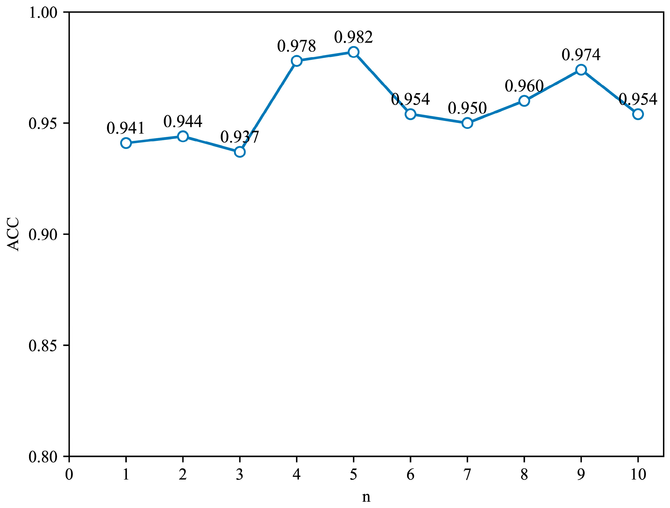
Furthermore, we choose the value of the number of hops n. At this time, the structural feature vector of the graph node is composed of the centrality measure and the number of neighboring nodes within n hops. Based on a graph convolutional network with 4 graph convolutional layers and 64 nodes in each layer, experiments were performed on the number of hops n in the range of 1 to 10, and the results are shown in Figure 7. It can be seen that the best detection accuracy of 98.2% is obtained when the value of n is 5

Figure 7. The detection accuracy of different hops.

In summary, the answer to question 1 is that the structure of the graph convolutional layer is determined to be 4 layers with 64 nodes for each, and the value of the hop number n is 5, so the graph node feature vector is composed of two centrality measures and the number of adjacent nodes within 5 hops.

(2) Question 2: Compared with the three existing approaches, namely the approach [5] of using permission combinations as features, the approach [17] of using API combinations as features and the approach [15] of embedding graphs into vector space, how effective is the detection method proposed in this paper?

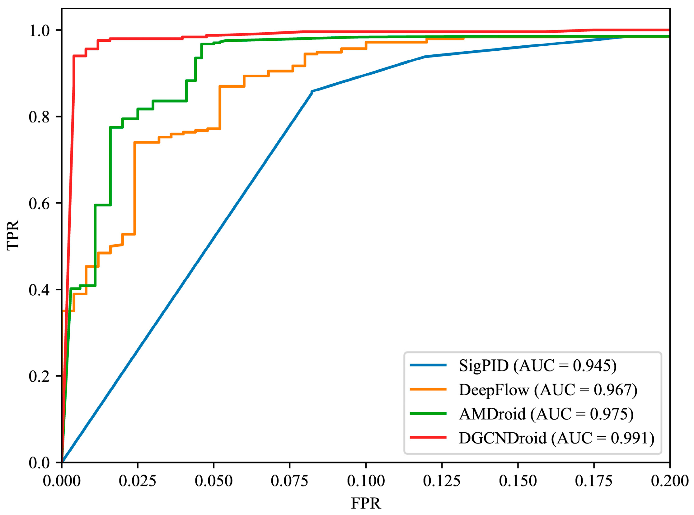
We compare DGCNDroid with the approach SigPID [5], which uses permission combination as a feature, DeepFlow [17], which uses API combination as a feature and AMDroid [15], an approach to embed graphs into a vector space. As shown in Table 6 and Figure 8.

Table 6. Comparison of DGCNDroid with three existing methods.

Approaches	ACC	TPR	FPR	AUC
SigPID [5]	0.938	0.968	0.091	0.945
DeepFlow [17]	0.964	0.948	0.020	0.967
AMDroid [15]	0.972	0.971	0.028	0.975
DGCNDroid	0.982	0.975	0.012	0.991

Figure 8. ROC curve of different methods.

It can be seen from Table 6 that DGCNDroid has a detection accuracy of up to 98% and a false positive rate of only 1.2%. Figure 8 shows the comparison of ROC curves between DGCNDroid, SigPID [5], DeepFlow [17] and AMDroid [15]. The ideal area under the ROC curve, in other words, AUC, is 1, so the closer the AUC area is to 1, the better the performance of the classifier. In the shape of the curve, the closer the inflection point of the curve is to the upper left corner, the higher the detection rate is and the lower the false positive rate is. It can be seen that compared with the ROC curves of the other three methods, the ROC curve of DGCNDroid is closer to the upper left corner, so it is more sensitive to malware detection and can better identify malware than other methods. At the same time, the curve of DGCNDroid is above the other three curves, so the area under the curve of DGCNDroid is significantly higher than that of the other three methods, which means that the DGCNDroid has a larger area under the curve.

In summary, the answer to Question 2 is that compared with the other three existing approaches, the approach in this paper has higher detection accuracy, recall rate and lower false positive rate, so the detection effect is better.

(3) Question 3: Can the approach of this paper be applied to multi-classification of malicious families, and how effective is the classification?

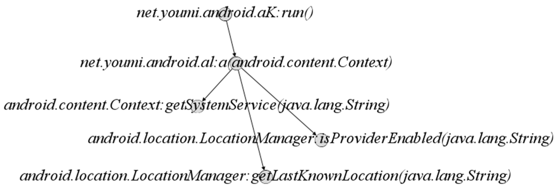
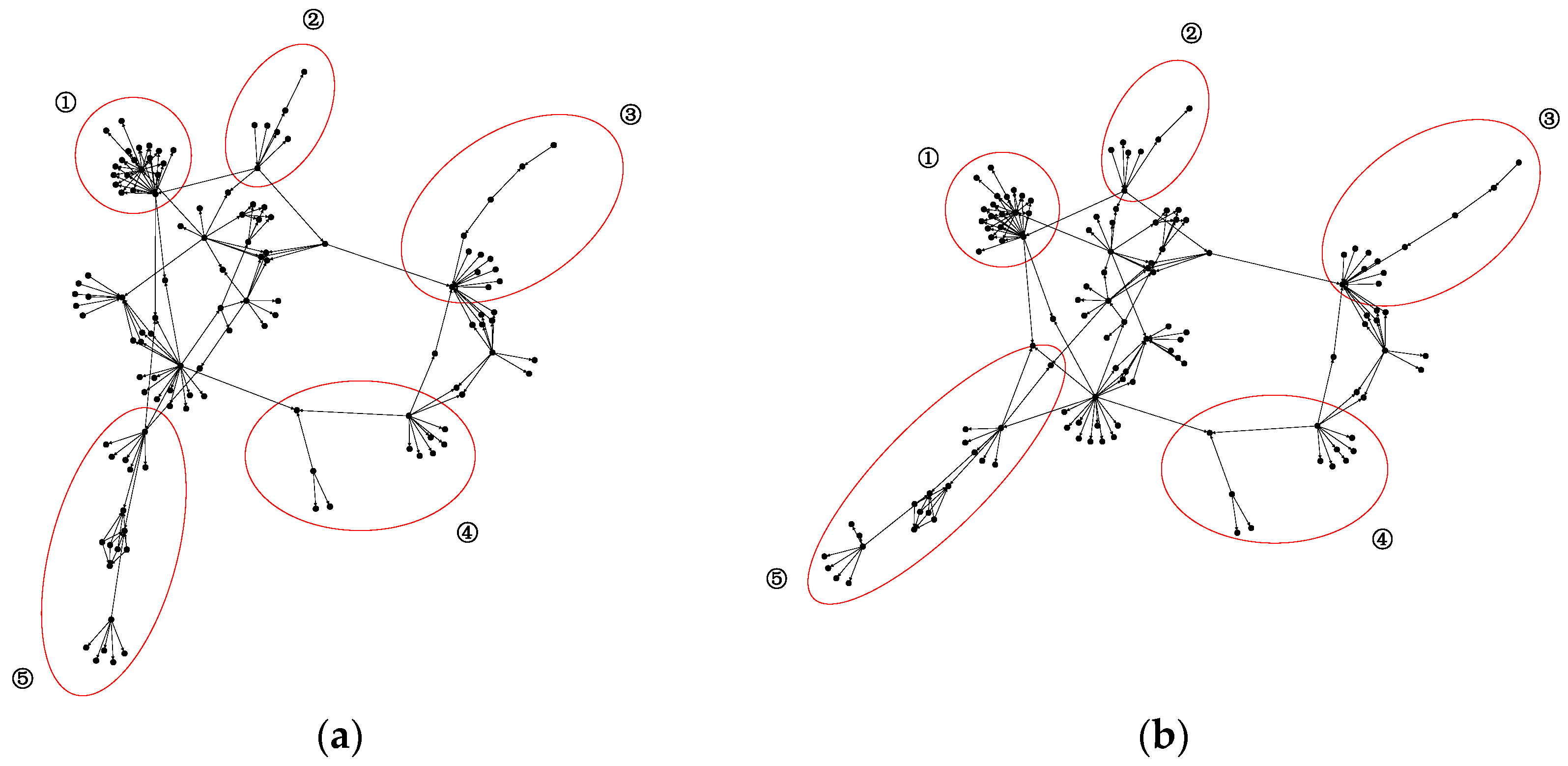
Although there are a large number of new malicious apps, most of them are variants of existing malicious applications. Malicious application developers usually use code reuse methods to modify or add new features based on the existing malicious application source code to achieve rapid release and cost reduction. Therefore, malicious applications will be aggregated in the form of families, and samples in the same family have similar malicious behaviors. As shown in Figure 9, malicious application (a) and application (b) belong to the family SndApp. Their malicious behavior is to obtain information such as device ID, email address and phone number and upload it to a remote server. By observing and comparing their function call graphs in Figure 9, it can be found that the two have a high similarity in the structure of the corresponding parts with the same number circled in red. Therefore, given that DGCNDroid can capture the structural features of the function call graph, we also conducted experiments on its multi-classification of malicious application families.

Figure 9. Similarity of function call graph structure of two malicious apps in SndApp family.

In order to compare with the results of the malicious family classification methods in literature [14] and literature [35], we utilize the same Android Malware Genome Project dataset [36] that is part of Drebin dataset [16] and contains 1260 applications from 49 families. For multi-classification, families containing only one sample need to be removed, and finally the dataset retains 1244 apps from 33 families. During training, the samples are sampled in a stratified manner at a ratio of 50%, and the remaining 50% of the samples are used for classification testing. When training the multi-classification model, the training samples are divided into 33 categories from 0 to 32. The structure of the deep graph convolutional network still follows the structure discussed in the binary classification, but the difference is that the final softmax output nodes are changed from 2 to 33. The macro accuracy is used to measure the classification effect on test set. The results are shown in Table 7.

Table 7. Multiple classification results of different approaches.

Approaches	Accuracy
FalDroid [14]	0.972
Dendroid [35]	0.942
DGCNDroid	0.969

Compared with approach [14] and approach [35] using the same data set, DGCNDroid achieves higher classification accuracy than the approach Dendroid [35] based on code structure mining. The classification effect of approach [14] is slightly better than that of DGCNDroid, but FalDroid [14] takes an average of 4.6 s to extract the graph features of an application [14], and it takes an average of 3.9 s to extract the features of an application using the approach of this paper. Therefore, the approach in this paper is better in terms of time overhead than approach [14].

In summary, the answer to question 3 is that the method in this article can also be applied to multi-classification of malicious families. The classification effect is close to the current advanced methods, but the time cost of feature extraction is better than the existing approaches.

5. Conclusions

This paper applies the deep graph convolutional network to Android malicious application detection, and proposes a malicious application detection method DGCNDroid based on the structural features of the function call graph. This method extracts the function call graph with sensitive API from the application, calculates the structural feature vector of the nodes in the graph, trains the extracted features through the deep graph convolutional network and retains more complete graph structure information. Through experiments on 11,120 application data sets, the method proposed in this paper has an accuracy rate of 98.2% in malicious application detection, which is better than other detection methods. At the same time, in the multi-classification of malicious application families, the method in this paper has also achieved a classification effect close to the advanced method. Because the method used in this article is a static analysis method, it will inevitably be affected by software hardening and code obfuscation, and it lacks effective handling of reflection and dynamic code loading. In the future, we will combine it with dynamic analysis methods to achieve comprehensive detection of Android malicious applications.

References

1. Smartphone Market Share. Available online: https://www.idc.com/promo/smartphone-market-share/os (accessed on 22 August 2020).
2. Android Passes 2.5 Billion Monthly Active Devices. Available online: https://venturebeat.com/2019/05/07/android-passes-2-5-billion-monthly-active-devices/ (accessed on 30 October 2020).
3. Mobile Cyber Threats. Available online: https://media.kaspersky.com/pdf/Kaspersky-Lab-KSN-Report-mobile-cyberthreats-web.pdf (accessed on 20 August 2020).
4. Mobile Phone Security Status Report of 2019. Available online: http://zt.360.cn/1101061855.php?dtid=1101061451&did=610435085 (accessed on 20 August 2020).
5. Li, J.; Sun, L.; Yan, Q.; Li, Z.; Srisa-An, W.; Ye, H. Significant Permission Identification for Machine-Learning-Based Android Malware Detection. IEEE Trans. Ind. Inform. 2018, 14, 3216–3225. [Google Scholar] [CrossRef]
6. Sokolova, K.; Perez, C.; Lemercier, M. Android Application Classification and Anomaly Detection with Graph-Based Permission Patterns. Decis. Support Syst. 2017, 93, 62–76. [Google Scholar] [CrossRef]
7. Song, J.; Han, C.; Wang, K.; Zhao, J.; Ranjan, R.; Wang, L. An Integrated Static Detection and Analysis Framework for Android. Pervasive Mob. Comput. 2016, 32, 15–25. [Google Scholar] [CrossRef]
8. Dai, G.; Ge, J.; Cai, M.; Xu, D.; Li, W. Svm-Based Malware Detection for Android Applications. In Proceedings of the 8th ACM Conference on Security & Privacy in Wireless and Mobile Networks, New York, NY, USA, 22 June 2015; pp. 1–2. [Google Scholar]
9. Liu, Z.; Lai, Y.; Chen, Y. Android Malware Detection Based on Permission Combinations. Int. J. Simul. Process. Model. 2015, 10, 315–326. [Google Scholar] [CrossRef]
10. Yusof, M.; Saudi, M.M.; Ridzuan, F. A New Mobile Botnet Classification Based on Permission and API Calls. In Proceedings of the 2017 Seventh International Conference on Emerging Security Technologies (EST), Canterbury, UK, 6–8 September 2017; pp. 122–127. [Google Scholar]
11. Zhu, J.; Wu, Z.; Guan, Z.; Chen, Z. API Sequences Based Malware Detection for Android. In Proceedings of the 2015 IEEE 12th Intl Conf on Ubiquitous Intelligence and Computing and 2015 IEEE 12th Intl Conf on Autonomic and Trusted Computing and 2015 IEEE 15th Intl Conf on Scalable Computing and Communications and Its Associated Workshops (UIC-ATC-ScalCom), Beijing, China, 10–14 August 2015; pp. 673–676. [Google Scholar]
12. Martín, A.; Menéndez, H.D.; Camacho, D. MOCDroid: Multi-Objective Evolutionary Classifier for Android Malware Detection. Soft Comput. 2017, 21, 7405–7415. [Google Scholar] [CrossRef]
13. Pei, X.; Yu, L.; Tian, S. AMalNet: A Deep Learning Framework Based on Graph Convolutional Networks for Malware Detection. Comput. Secur. 2020, 101792. [Google Scholar] [CrossRef]
14. Fan, M.; Liu, J.; Luo, X.; Chen, K.; Tian, Z.; Zheng, Q.; Liu, T. Android Malware Familial Classification and Representative Sample Selection via Frequent Subgraph Analysis. IEEE Trans. Inf. Forensics Secur. 2018, 13, 1890–1905. [Google Scholar] [CrossRef]
15. Ge, X.; Pan, Y.; Fan, Y.; Fang, C. AMDroid: Android Malware Detection Using Function Call Graphs. In Proceedings of the 2019 IEEE 19th International Conference on Software Quality, Reliability and Security Companion (QRS-C), Sofia, Bulgaria, 22–26 July 2019; pp. 71–77. [Google Scholar]
16. Arp, D.; Spreitzenbarth, M.; Hubner, M.; Gascon, H.; Rieck, K.; Siemens, C. Drebin: Effective and Explainable Detection of Android Malware in Your Pocket. In Proceedings of the Network and Distributed System Security Symposium (NDSS), San Diego, CA, USA, 23–26 February 2014; Volume 14, pp. 23–26. [Google Scholar] [CrossRef]
17. Zhu, D.; Jin, H.; Yang, Y.; Wu, D.; Chen, W. DeepFlow: Deep Learning-Based Malware Detection by Mining Android Application for Abnormal Usage of Sensitive Data. In Proceedings of the 2017 IEEE Symposium on Computers and Communications (ISCC), Heraklion, Greece, 3–6 July 2017; pp. 438–443. [Google Scholar]
18. Li, D.; Wang, Z.; Xue, Y. Fine-Grained Android Malware Detection Based on Deep Learning. In Proceedings of the 2018 IEEE Conference on Communications and Network Security (CNS), Beijing, China, 30 May–1 June 2018; pp. 1–2. [Google Scholar]
19. Xu, K.; Li, Y.; Deng, R.H.; Chen, K. Deeprefiner: Multi-Layer Android Malware Detection System Applying Deep Neural Networks. In Proceedings of the 2018 IEEE European Symposium on Security and Privacy (EuroS&P), London, UK, 24–26 April 2018; pp. 473–487. [Google Scholar]
20. Taheri, R.; Ghahramani, M.; Javidan, R.; Shojafar, M.; Pooranian, Z.; Conti, M. Similarity-Based Android Malware Detection Using Hamming Distance of Static Binary Features. Future Gener. Comput. Syst. 2020, 105, 230–247. [Google Scholar] [CrossRef]
21. Liang, H.; Song, Y.; Xiao, D. An End-to-End Model for Android Malware Detection. In Proceedings of the 2017 IEEE International Conference on Intelligence and Security Informatics (ISI), Beijing, China, 22–24 July 2017; pp. 140–142. [Google Scholar]
22. Shabtai, A.; Kanonov, U.; Elovici, Y.; Glezer, C.; Weiss, Y. “Andromaly”: A Behavioral Malware Detection Framework for Android Devices. J. Intell. Inf. Syst. 2012, 38, 161–190. [Google Scholar] [CrossRef]
23. Hou, S.; Saas, A.; Chen, L.; Ye, Y. Deep4maldroid: A Deep Learning Framework for Android Malware Detection Based on Linux Kernel System Call Graphs. In Proceedings of the 2016 IEEE/WIC/ACM International Conference on Web Intelligence Workshops (WIW), Omaha, NE, USA, 13–16 October 2016; pp. 104–111. [Google Scholar]
24. Ananya, A.; Aswathy, A.; Amal, T.R.; Swathy, P.G.; Vinod, P.; Mohammad, S. SysDroid: A Dynamic ML-Based Android Malware Analyzer Using System Call Traces. Clust. Comput. 2020, 23, 2789–2808. [Google Scholar] [CrossRef]
25. Alshahrani, H.; Mansourt, H.; Thorn, S.; Alshehri, A.; Alzahrani, A.; Fu, H. DDefender: Android Application Threat Detection Using Static and Dynamic Analysis. In Proceedings of the 2018 IEEE International Conference on Consumer Electronics (ICCE), Berlin, Germany, 12–14 January 2018; pp. 1–6. [Google Scholar]
26. Yuan, Z.; Lu, Y.; Wang, Z.; Xue, Y. Droid-Sec: Deep Learning in Android Malware Detection. In Proceedings of the 2014 ACM Conference on SIGCOMM, Chicago, IL, USA, 19 August 2014; pp. 371–372. [Google Scholar]
27. Saracino, A.; Sgandurra, D.; Dini, G.; Martinelli, F. MADAM: Effective and Efficient Behavior-Based Android Malware Detection and Prevention. IEEE Trans. Dependable Secur. Comput. 2018, 15, 83–97. [Google Scholar] [CrossRef]
28. Estrach, J.B.; Zaremba, W.; Szlam, A.; LeCun, Y. Spectral Networks and Deep Locally Connected Networks on Graphs. In Proceedings of the 2nd International Conference on Learning Representations, Banff, AB, Canada, 14–16 April 2014. [Google Scholar]
29. Defferrard, M.; Bresson, X.; Vandergheynst, P. Convolutional Neural Networks on Graphs with Fast Localized Spectral Filtering. In Proceedings of the 30th International Conference on Neural Information Processing Systems, Barcelona, Spain, 30 April 2016; pp. 3844–3852. [Google Scholar]
30. Kipf, T.N.; Welling, M. Semi-Supervised Classification with Graph Convolutional Networks. In Proceedings of the 5th International Conference on Learning Representations, Toulon, France, 24–26 April 2017. [Google Scholar]
31. Zhang, M.; Cui, Z.; Neumann, M.; Chen, Y. An End-to-End Deep Learning Architecture for Graph Classification. In Proceedings of the AAAI Conference on Artificial Intelligence, New Orleans, LA, USA, 2–7 February 2018; Volume 18, pp. 4438–4445. [Google Scholar]
32. Hamilton, W.; Ying, Z.; Leskovec, J. Inductive Representation Learning on Large Graphs. In Proceedings of the Advances in Neural Information Processing Systems, Long Beach, CA, USA, 4–9 December 2017; pp. 1024–1034. [Google Scholar]
33. Niepert, M.; Ahmed, M.; Kutzkov, K. Learning Convolutional Neural Networks for Graphs. In Proceedings of the International Conference on Machine Learning, New York, NY, USA, 19–24 June 2016; pp. 2014–2023. [Google Scholar]
34. Backes, M.; Bugiel, S.; Derr, E.; McDaniel, P.; Octeau, D.; Weisgerber, S. On Demystifying the Android Application Framework: Re-Visiting Android Permission Specification Analysis. In Proceedings of the 25th USENIX Security Symposium (USENIX Security 16), Austin, TX, USA, 10–12 August 2016; pp. 1101–1118. [Google Scholar]
35. Suarez-Tangil, G.; Tapiador, J.E.; Peris-Lopez, P.; Blasco, J. Dendroid: A Text Mining Approach to Analyzing and Classifying Code Structures in Android Malware Families. Expert Syst. Appl. 2014, 41, 1104–1117. [Google Scholar] [CrossRef]
36. Zhou, Y.; Jiang, X. Dissecting Android Malware: Characterization and Evolution. In Proceedings of the 2012 IEEE Symposium on Security and Privacy, Francisco, CA, USA, 24–25 May 2012; pp. 95–109. [Google Scholar]
Publisher’s Note: MDPI stays neutral with regard to jurisdictional claims in published maps and institutional affiliations.
Article Metrics
Citations
Article Access Statistics
Multiple requests from the same IP address are counted as one view.