Article

Parallel Multiphysics Simulation of Package Systems Using an Efficient Domain Decomposition Method

1
Institute of Applied Physics and Computational Mathematics, Beijing 100088, China
2
Software Center for High Performance Numerical Simulation of CAEP, Beijing 100088, China
*
Author to whom correspondence should be addressed.
Electronics 2021, 10(2), 158; https://doi.org/10.3390/electronics10020158
Submission received: 1 December 2020 / Revised: 24 December 2020 / Accepted: 7 January 2021 / Published: 13 January 2021
(This article belongs to the Special Issue High-Performance Computer Architectures and Applications)

Abstract

:
With the continuing downscaling in feature sizes, the thermal impact on material properties and geometrical deformations can no longer be ignored in the analysis of the electromagnetic compatibility or electromagnetic interference of package systems, including System-in-Package and antenna arrays. We present a high-performance numerical simulation program that is intended to perform large-scale multiphysics simulations using the finite element method. An efficient domain decomposition method was developed to accelerate the multiphysics loops of electromagnetic–thermal stress simulations by considering the fact that the electromagnetic field perturbations caused by geometrical deformation are small and constrained in one or a few subdomains. The multi-level parallelism of the algorithm was also obtained based on an in-house developed parallel infrastructure. Numerical examples showed that our algorithm is able to enable simulation with multiple processors in parallel and, more importantly, achieve a significant reduction in computation time compared with traditional methods.

1. Introduction

Multifunctional integration and miniaturization are the developing directions of modern electronic systems [1,2,3]. These electronic systems are always integrated with high-density passive devices or interconnects, where signal delay, reflection, attenuation, and crosstalk have become the dominant factors limiting overall performance with the continuing downscaling in feature sizes and increasing in operating frequency [4,5,6,7]. When multiphysics field effects emerge, traditional simulations cannot adequately handle new challenges of various electromagnetic, thermal, and mechanical effects, especially the joule heating effects caused by increases of input power. Electromagnetic-induced heat generation and resulting elevated temperatures adversely affect the performance and reliability of these devices. All these challenging issues are pushing the transition from traditional electromagnetic simulations to multiphysics simulations of package systems. Multiphysics analysis tools of commercial software, like ANSYS WORKBENCH and COMSOL, can handle the multiphysics simulations of electronic elements like antennas or waveguides but not for electronic systems. Related literature on efficient system-level multiphysics modes [8,9], where electromagnetic models and thermal resistance models were developed, has been published. However, neither the size effects of package systems with high operating frequency nor the mechanical effects have been considered during multiphysics simulations.
Full-wave electromagnetic simulations of such systems have been conducted by numerical methods and their parallel algorithms such as the finite element method (FEM) [10], the method of moments (MoM) [11], and the finite difference time domain (FDTD) method [12]. However, for practical package systems, these structures pose immense challenges for existing numerical methods like MoM and FDTD. Many papers have been published with the FEM thanks to its flexibility in geometric and material manipulation. Considering the ill-conditioning feature of the FEM matrix in electromagnetic simulation, the recently developed domain decomposition method (DDM) [13,14,15], iterative class and hierarchical matrix method [16], and direct class methods are thought to provide effective ways to conquer the solving problems of FEM matrix equations. A previous study [14] proposed a double-level parallel scheme of the FEM to achieve the solving of over three billion unknowns on 9600 CPU cores, though only for electromagnetic simulation. Additionally, many investigations have been done to numerically analyze multiphysics effects on the operating state of package systems [17,18], including this paper’s authors’ recent work [19]. However, that work [19] did not consider thermal or mechanical impact on electrical performance. Furthermore, even with the newly developed methods, hundreds of iterations are always needed in large-scale problems, which makes it difficult to conduct the multiphysics simulation of real-life package systems, where electromagnetic solving always takes a couple of hours and is unaffordable.
Considering the fact that similar problems are solved several times during multiphysics simulations, it is necessary to improve the efficiency of repeated computing where there are mesh deformation/morphing techniques [20,21,22]. In this approach, an existing mesh can be smoothly transformed to conform the geometrical modification caused by thermal strains. However, a linear system requires solving to update the mesh. Considering that a simulated system is electrically small within the interested frequency band, the authors of [23] suggested recycling the Krylov subspace to reduce the total number of iterations. A novel embedded DDM was also presented for repeated electromagnetic modeling in designs while considering the geometrical and material differences between subdomains [24]. In fact, the embedded DDM is a kind of method that employs the background field as the initial guess of new linear-system, and a large number of unknowns are introduced because there are overlapping areas between subdomains and background domain.
In this paper, we propose an efficient parallel multiphysics simulation strategy. A non-overlapping DDM was used to compute an electromagnetic field, and then thermal and stress computations were conducted to update the temperature, material properties, and geometrical deformations, thus forming a multiphysics simulation loop. Here, instead of a background electromagnetic field, an efficient interpolation by means of subdomain boundary values could be used to obtain much faster convergence of electromagnetic computing, which finally accelerated the whole multiphysics simulations by several times. Mathematically, this method is an efficient implementation of MOR (mode order reduction) by means of the DDM, and the motivation of our work came from the fact that the change of the solving/searching space is quite small during repeated computing. Physically, the geometrical deformation of package systems has little influence on the whole electromagnetic distribution but does have influence on the regions surrounding them. High-order modes of electromagnetics can only propagate across few adjacent sub-domains. Therefore, subdomain boundary values can give a good estimation of change. Furthermore, the multi-level parallelism of the algorithm were also obtained based on an in-house developed infrastructure JAUMIN (J Parallel Adaptive Unstructured Mesh Applications Infrastructure) [25]. Numerical examples with millions of unknowns are presented to prove our theorem and show the performance of the proposed parallel algorithm.
The remainder of the paper is organized as follows: Section 2 describes the mathematical model of our multiphysics problems. Section 3 presents the parallel implementation including an in-house developed parallel infrastructure and a parallel scheme of the multiphysics simulation method. A validation example and two real-life numerical examples of the proposed work are discussed in Section 4. Section 5 concludes the paper.

2. Mathematical Implementation

2.1. Boundary Value Problem of Electromagnetic Field

We start by reviewing the Helmholtz equation defined in an open region Ω . A Silver-Müller radiation condition is used to truncate the infinite domain. This leads to the following problem:
{ × ( μ r 1 × E ) k 0 2 ε r E = j ω μ 0 J imp in   Ω γ t ( E ) = 0 on   Ω Γ PEC γ t ( μ r 1 × E ) + j k γ T ( E ) = 0 on   Ω Γ [ [ μ r 1 × E ] ] × = j k η J port on   Γ port
where E is the electric field with a unit of V / m , J is the current density with a unit of A / m 3 , ε r = ε / ε 0 is the relative permittivity, and μ r = μ / μ 0 is the relative permeability with ε 0 = 8.85   ×   10 12   ( F / m ) and μ 0 = 4 π   ×   10 7 ( H / m ) . ω is the angular frequency with a unit of rad / s , k = ω μ 0 ε 0 is the wavenumber, and j = 1 is the imaginary unit. The free-space intrinsic impedance is denoted as η = μ 0 / ε 0 , and the tangential trace and the tangential component trace operators for any vector v are given by γ T ( v ) : v n × v × n and γ t ( v ) : v n × v , respectively, where n is the unit vector outwardly oriented normal to Ω . [ [ v ] ] × : = γ t + ( v + ) γ t ( v ) refers to the associated field jump across a surface. An efficient DDM solver is used to solve the electromagnetic problems, and its implementation is described in the following section.

2.2. Electromagnetic–Thermal Stress Coupling

Consider a domain Ω in which an electromagnetic field is calculated; the governing equations for the steady thermal system are given by
{ ( κ T ) = Q e   in Ω k n T n | Γ C = h ( T T a ) | Γ C on Γ C T | Γ T = T b on Γ T
where T is the temperature with a unit of K , κ is the thermal conductivity with unit a unit of W / ( K m ) , and h is the thermal convection coefficient with a unit of W / ( K m 2 ) . The heat source represents the electromagnetic losses Q e ( W / m 3 ) and is given by
Q e = Q r h + Q m l
where the resistive losses are
Q r h = 1 2 Re ( J E * )
and the magnetic losses are
Q m l = 1 2 Re ( j ω B H * )
where H is the magnetic field with a unit of A / m and B is the magnetic flux density with a unit of T . In addition, this equation maps the electromagnetic surface losses of the conductors as a heat source on the boundary
Q e = 1 2 | J S | 2 Re ( Z S )
where J S represents the surface electric current and Z S represents the surface impedance.
The governing equation of the thermal stress simulation was derived according to both Hooke’s and Newton’s laws, as given by
{ [ ] T σ + f = 0   in   Ω σ = D ( [ ] U ε T )   in   Ω U | Γ U = U ¯   on   Γ u σ i j n j | Γ σ = λ ¯ i   on   Γ σ
in which σ = [ σ x σ y σ z σ x y σ y z σ z x ] T is the stress vector and f is the volume force. U = [ u x u y u z ] T , and u x , u y , and u z are the structural displacements at the x , y , and z directions, respectively. [ ] is a differential operator matrix defined as
[ ] T = [ / x / y / z / y / x / z / z / y / x ]
D is the elastic constant tensor with element
D i j k l = E ( T ) 1 + υ δ i k δ j l + E ( T ) υ ( 1 + υ ) ( 1 2 υ ) δ i k δ j l
and in Equation (7),
ε T = [ α Δ T α Δ T α Δ T 0 0 0 ] T
is the thermal strain, in which α is named as the coefficient of thermal expansion with a unit of 1 / K , and Δ T is the temperature variation obtained by solving the heat conduction equation.

3. DDM Solver and Parallel Implementation

3.1. DDM Solver and Multiphysics Simulations

To directly implement the DDM, a generalized Schwarz algorithm of Equation (1) is used for two subdomains Ω = Ω 1 Ω 2 ; it then solves them in an iterative way for n = 1 ,   2 ,   ,   and   N , respectively, i.e.,
× 1 μ r × E 1 n k 0 2 ε r E 1 n = j ω μ 0 J 1   in   Ω 1
Τ n 1 ( E 1 n ) = Τ n 1 ( E 2 n 1 )   on   Γ 12
× 1 μ r × E 2 n k 0 2 ε r E 2 n = j ω μ 0 J 2   in   Ω 2
Τ n 2 ( E 2 n ) = Τ n 2 ( E 1 n 1 )   on   Γ 21
where Γ 12 = Ω 1 Ω 2 , Γ 21 = Ω 2 Ω 1 , Τ n j represents the transmission condition, and n j denotes the unit outward normal vector of the subdomain Ω j . The transmission condition can be written as
Τ n ( E ) = ( I + ( δ 1 S T M + δ 2 S T E ) ) ( γ t ( E ) ) j ω ε μ ( I ( δ 3 S T M + δ 4 S T E ) ) ( γ T ( E ) )
where S T M = τ τ , S T E = τ × τ × , τ denotes the tangential direction, and δ l   ( l = 1 ,   2 ,   3 ,   and   4 ) are the parameters for different transmission conditions.
The DDM with non-overlapping region requires a matching grid between two adjacent subdomains. The computational domain is at first meshed and decomposed into M equivalent-size subdomains automatically by the in-house developed parallel infrastructure JAUMIN. Each subdomain has a ghost region that extends several grids into its neighboring domains. The ghost region can facilitate the implementation of the DDM. On each subdomain, we define discrete trial and test functions as u m h , v m h X m h H ( c u r l ; Ω m ) ; when order p = 0 , there are 6 vector basis functions within each tetrahedron. The final weak form of the DDM with the Robin transmission condition can be interpreted by the following equations, with the absorbing boundary condition implementation neglected:
Seek ( u i h , u j h ) X i h × X j h , and
( × v 1 h , μ r 1 1 × u 1 h ) κ 1 k 0 2 ( v 1 h , ε r 1 u 1 h ) κ 1 + k 0 v 1 h , μ r 1 1 γ t ( × u 1 h ) Γ 12 = j ω μ 0 ( v 1 h , J ) κ 1   in   Ω 1
( × v 2 h , μ r 2 1 × u 2 h ) κ 2 k 0 2 ( v 2 h , ε r 2 u 2 h ) κ 2 + k 0 v 2 h , μ r 2 1 γ t ( × u 2 h ) Γ 21 = j ω μ 0 ( v 2 h , J ) κ 2   in   Ω 2
v 1 h , μ r 1 1 γ t ( × u 1 h ) j k 0 v 1 h , γ t ( u 1 h × n ) = v 1 h , μ r 2 1 γ t ( × u 2 h ) j k 0 v 1 h , γ t ( u 2 h × n )   on   Γ 12
v 2 h , μ r 2 1 γ t ( × u 2 h ) j k 0 v 2 h , γ t ( u 2 h × n ) = v 2 h , μ r 1 1 γ t ( × u 1 h ) j k 0 v 2 h , γ t ( u 1 h × n )   on   Γ 21
Here, we define the volume and surface integral forms by ( u , v ) Ω : = Ω u ¯ v d v and u , v Ω : = Ω u ¯ v d s , where the over bar denotes the conjugation. The parameters in Equation (13) are set to be δ l = 0   ( l = 1 ,   2 ,   3 ,   and   4 ) . The unit normal vector n of the interface boundary Γ i j is pointing away from the subdomain Ω i . The matrix equation resulting from the above formulas can be further written in a compact form, and for the case of two subdomains, we have
[ A 1 C 12 C 21 A 2 ] [ u 1 u 2 ] = [ y 1 y 2 ]
where the matrices A 1 and A 2 are subdomain matrices respectively following the two interface coupling matrices C 12 and C 21 .
It is instructive to first consider the thermal strain in Equation (10) of a material with a maximum thermal expansion, which is usually copper with α = 1.65 × 10 5 in package systems. Thus, an estimation of 1.0 × 10⁻³ m of the largest geometrical deformation is reasonable during the operating state of systems. This geometrical deformation is far less than the wavelength of interest. Therefore, geometrical deformation has little influence on the electromagnetic distribution of a whole region but does have influence on those subdomains surrounding the deformation. This is mainly due to the fact that the high-order modes of electromagnetic interference can only propagate across few adjacent sub-domains. As a result, the DDM can get very fast convergence with the interpolation of subdomain boundary values. The strategy of the DDM accelerating multiphysics simulation is illustrated as Algorithm 1.
Algorithm 1. Multiphysics loops based on the domain decomposition method (DDM)
  Initial electromagnetic guess u 0 = 0 ,   Λ 0 n = 0 and set p = 0
  Do
    Assemble linear system: A p u p = b p
    Solve: u p = DDMsolver ( A p , Λ p , b p )
    Update boundary value: Λ p T n ( u p )
    Thermal stress computing
    Update material properties and grid coordinates
    Update: p = p + 1
  While
    Multiphysics loops not converged
p: multiphysics loops; n: sub-domain number  

3.2. Parallel Infrastructure and Parallel Algorithm

JAUMIN is an in-house developed programming framework for massively parallel numerical simulations on unstructured meshes. It facilitates the development of large-scale parallel unstructured-mesh applications, and it supports applications to scale to tens of thousands of CPU cores. As shown in Figure 1, the geometry is discretized into a mesh level and then subdivided into subdomains. These subdomains are assigned to computing nodes of the supercomputer and exchange data through explicit MPI calls. Within each of nodes, the domain is further divided into smaller sub-domains called regions. The regions are bound to CPU sockets and communicate with each other through non-uniform memory access (NUMA)-aware message passing or multi-threading. In each of CPU sockets, the region is finally divided into patches. Usually, one patch is assigned to one core. The data communications among patches are implemented by multi-threading. In the CPU core, the mesh cells are transferred into the private cache, and SIMD parallelization can be implemented.
The proposed multi-level parallel scheme of Algorithm 1 is presented in Figure 2. As indicated above, after reading the mesh, JAUMIN generates patch hierarchies and distributes them to every process according to the inherent workload distribution scheme. To make sure that parallel processes do equal amounts of work, spatial locality can also be addressed with dynamic scheduling by defining a minimum number of the successive subdomains assigned to each process. The DDMSolver in Algorithm 1 is marked with a red line. The subsystem in a patch is solved individually by a direct method and parallelized among the threads. Once the electromagnetic solving is finished, a thermal stress coupling system is constructed and solved by calling the parallel linear solver.

4. Numerical Examples

We now examine the performance of our proposed multiphysics algorithm by validating its efficiency. During all the numerical experiments, the stopping criterion of the electromagnetic DDMSolver was set to be the residual reduced by a factor of 1.0 × 10⁻³ if no particular indication was used. We note that a maximum number of 16 multiphysics loops were always performed in our program to make sure the temperature change between two adjacent multiphysics loops was less than 0.1 K; thus, the convergence of multiphysics simulation was achieved. Furthermore, the multiphysics system was built in parallel, and a parallel Portable, Extensible Toolkit for Scientific Computation (PETSc) library [26] was employed to solve the linear system. Specifically, the sub-linear systems of the DDM were solved by the PETSc library associated with the MUltifrontal Massively Parallel Sparse Direct Solver (MUMPS) [27]. The linear systems of thermal stress coupling systems were solved by a GMRES solver with an AMG preconditioner from the HYPRE library [28].
A type of computer platform with NUMA architecture was used to acquire the simulated results, i.e., TS10K cluster, which is designed and manufactured by INSPUR Co., Ltd. JINAN, CHINA. This platform is equipped with 57 compute nodes and each one has two CPUs with the following specifications: Intel Xeon E5-2692V2 (2.20GHz/12cores)/8.0GT/30ML3/1866, 32G ECC Registered DDR3 1600 RAM, Linux Enterprise 6.3 X64 with kernel 2.6.32-279.e16.x86_64.

4.1. Numerical Validation

Our beginning simulation was to validate the accuracy of our program using an antenna element with an operating frequency of 3.0 GHz and an input power of 50 W. A number of 503,370 grids were generated, and 12 CPU cores were used for 12 sub-domains to process the DDM iterations. Specifically, absorbing boundary conditions for the electromagnetic simulation were applied, and a wave port was used to excite the antenna. For the thermal simulation, all boundaries exterior to the air were set as thermal convection boundaries with h = 5   W / ( K m 2 ) and T a = 298.15   K . For the stress simulation, the bottoms of the antennas were fixed with U = [ 0 0 0 ] T . The calculated highest temperature had a good agreement with that of the commercial software ANSYS, as listed in Table 1. Figure 3 shows the geometrical details and calculated temperature distribution.

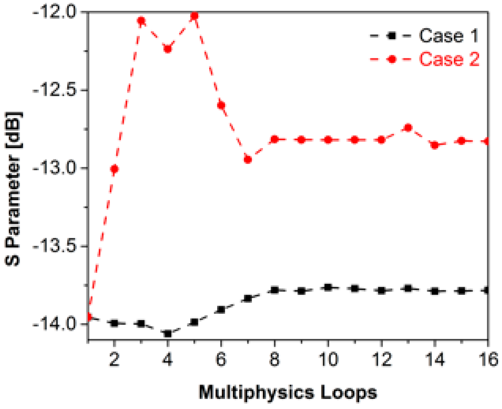
4.2. Multiphysics Simulation of Real-Life System-In-Package

As shown in Figure 4, we then considered a real-life System-in-Package. It was stacked with 12 boards consisting of high-density interconnects and a total number of 4800 entities, with a minimum size of 10   μ m and a whole size of over 10 mm. A number of 5,830,000 girds were generated, and 140 CPU cores were used to perform the multiphysics simulations. Specifically, absorbing boundary conditions for electromagnetic simulation were applied, and a lumped port was used to excite the simulation. For the thermal simulation, all boundaries exterior to the air are set as thermal convection boundaries with h = 5   W / ( K m 2 ) and T a = 298.15   K . For the stress simulation, the bottom of the substrate was fixed with U = [ 0 0 0 ] T .
The calculated results are summarized in Table 2. The multiphysics simulation procedure and the calculated maximum temperature values of two simulation cases are demonstrated in Figure 5 and Figure 6, respectively. The convergence of the S parameters is shown in Figure 7, and this parameter was defined as S = V V i n / V i n , where V is the voltage of the port. It is worth noting that this real-life System-in-Package cost the DDMSolver 468 iterations to converge at the first multiphysics simulation loop. Fortunately, the DDM iteration number dropped quickly for both cases with different microwave input power values. The results in Figure 5 and Figure 6 show that the algorithm performance did not degrade with larger geometrical deformation, and the total consuming time is shown in Table 2, with the last 15 multiphysics simulation loops only taking about 35% of the total computing time. It is reasonable to note that the slower convergence was always with the larger input power, i.e., larger temperature variation and larger geometrical deformations. A deviation of 0.1 dB of the two cases can be seen when comparing Figure 5 and Figure 6. It was necessary to increase the input power, e.g., from 10.0 to 50.0 W with a step of 10.0 W, during the multiphysics simulations. The distributions of the electric, temperature, and strain fields are illustrated in Figure 8.

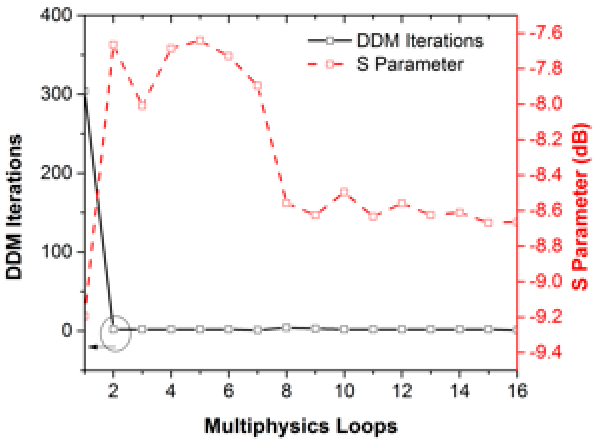
4.3. Multiphysics Simulation of Antenna Array and Radome

Our last numerical example was the multiphysics simulation of a real-life antenna array, as shown in Figure 9a, which consisted of 33 antenna elements and a multilayer radome attached by a frequency selective surface. Each antenna element was operating at a frequency of 2.6 GHz with an input power of 100.0 W. The geometrical scale reached a magnitude of three orders, leading to a total number of 96,800,000 grids and 125,846,630 unknowns for electromagnetic simulations, 12,883,936 unknowns for thermal simulations, and 38,651,808 unknowns for stress computing. We used 196 CPU cores for 3072 sub-domains to perform electromagnetic DDM iterations. Specifically, absorbing boundary conditions for electromagnetic simulation were applied, and 33 wave ports were used to excite the simulation. For the thermal simulation, all boundaries exterior to the air were set as thermal convection boundaries with h = 5   W / ( K m 2 ) and T a = 298.15   K . For the stress simulation, the bottom of the antennas and the top face of the radome were fixed with U = [ 0 0 0 ] T .
The multiphysics simulation information is illustrated in Table 3, and the simulation procedure is demonstrated in Figure 10. The simulation cost the DDMSolver 304 iterations to converge at the first multiphysics loop, and then the number of DDM iteration steps dropped quickly to around 5. The total consuming time was 64,965 s with the first loop of 58,468 s, and 935,468 s of 16 multiphysics loops were consumed when we used traditional methods. Thus, it is reasonable to evaluate our method as being 10 times faster than the traditional method. A final maximum temperature of 499.0 K and an S parameter of -8.66 dB of the first element were achieved. Additionally, the distributions of electric, temperature, and strain fields of the antenna array, together with the radome, are illustrated in Figure 9b–d, respectively.

5. Conclusions and Future Works

In this paper, we developed an efficient algorithm that could dramatically speed up multiphysics simulations by reusing of the solving space of the DDM. The multi-level parallelism of the proposed method was obtained based on an in-house developed parallel infrastructure called JAUMIN, which is able to solve large-scale problems with millions of unknowns. The optimal simulation efficiency was characterized by several numerical experiments, with a dramatic reduction of time-consumption compared with traditional methods.
Simulations of large-scale problems with over 100 million unknowns are needed to verify the advantages of the proposed method, and more research is needed to further reduce the execution time for larger problems, especially that of the first multiphysics loop. To do this, higher order transmission boundary conditions of the DDM can be developed to accelerate the convergence rate of electromagnetic solving. Moreover, investigations into extreme thermal conditions must be conducted when the temperature rise is significant and the geometrical deformation can be as large as 10 × 10−2 m. It was also indicated that with this strategy, more comprehensive design methods, especially geometrical optimization and frequency sweeping methods, can be further developed.

Author Contributions

Investigation, W.W. and Y.L.; software, W.W.; writing, W.W.; validation, Z.Z.; supervision, H.Z. All authors have read and agreed to the published version of the manuscript.

Funding

This work was supported and in part by National Natural Science Foundation of China (NSFC) under Grant 12001053, 61771061, in part by the Innovation Program of CAEP under Grant CX2019034, in part by the Science Challenge Project under Grant TZ2018002.

Informed Consent Statement

Informed consent was obtained from all subjects involved in the study.

Acknowledgments

We thank Wenyan Yin from Zhejiang University, for providing useful instructions.

Conflicts of Interest

The authors declare no conflict of interest.

References

  1. Carson, F.; Kim, Y.C.; Yoon, I.S. 3-D stacked package technology and trends. Proc. IEEE 2009, 97, 31–42. [Google Scholar] [CrossRef]
  2. Meindl, J.D. Beyond Moore’s Law: The interconnect era. IEEE Comput. Sci. Eng. 2003, 5, 20–24. [Google Scholar] [CrossRef]
  3. Lu, J.-Q. 3-D hyperintegration and packaging technologies for micronano systems. Proc. IEEE 2009, 97, 18–30. [Google Scholar] [CrossRef]
  4. Wane, S.; Kuo, A.-Y.; Santos, P.D. Dynamic power and signal integrity analysis for chip-package-board co-design and co-simulation. In Proceedings of the 2009 European Microwave Integrated Circuits Conference (EuMIC), Rome, Italy, 28–29 September 2009. [Google Scholar]
  5. Ong, C.-J.; Wu, B.P.; Tsang, L.; Gu, X. Full-wave solver for microstrip trace and through-hole via in layered media. IEEE Trans. Adv. Packag. 2008, 31, 292–302. [Google Scholar]
  6. Huang, C.-C.; Lai, K.L.; Tsang, L.; Gu, X.; Ong, C.-J. Transmission and scattering on interconnects with via structures. Microw. Opt. Technol. Lett. 2005, 46, 446–452. [Google Scholar] [CrossRef]
  7. Interconnect Application Note: Z-pack HM-Zd PWB Footprint Optimization for Routing. Report, 20GC015-1, Rev. B. July 2003. Available online: http://agata.pd.infn.it/LLP_Carrier/New_ATCA_Carrier_web/Assemby_Docs/footprint_optimization.pdf (accessed on 1 December 2020).
  8. Blair, C.; Ruiz, S.L.; Morales, M. 5G, a multiphysics simulations vision from antenna element design to system link analysis. In Proceedings of the IEEE ICEAA, Granada, Spain, 9–13 September 2019. [Google Scholar]
  9. Baptista, E.; Buisman, K.; Vaz, J.C.; Fager, C. Analysis of thermal coupling effects in integrated MIMO transmitters. In Proceedings of the IEEE MTT-S IMS, Honololo, HI, USA, 1–4 June 2017. [Google Scholar]
  10. Jin, J.-M. The Finite Element Method in Electromagnetics, 3rd ed.; Wiley: New York, NY, USA, 2014. [Google Scholar]
  11. Peng, Z.; Shao, Y.; Gao, H.W.; Wang, S.; Lin, S. High-Fidelity, High-Performance Computational Algorithms for Intrasystem Electromagnetic Interference Analysis of IC and Electronics. IEEE Trans. Compon. Packag. Technol. 2017, 7, 653–668. [Google Scholar] [CrossRef]
  12. Yan, J.; Jiao, D. Fast explicit and unconditionally stable FDTD method for electromagnetic analysis. IEEE Trans. Microw. Theory Tech. 2017, 65, 2698–2710. [Google Scholar] [CrossRef]
  13. Dolean, V.; Gander, M.J.; Lanteri, S.; Lee, J.-F.; Peng, Z. Effective transmission conditions for domain decomposition methods applied to the time-harmonic curl-curl Maxwell’s equations. J. Comput. Phys. 2015, 280, 232–247. [Google Scholar] [CrossRef] [Green Version]
  14. Wang, W.J.; Xu, R.; Li, H.Y.; Liu, Y.; Guo, X.-Y.; Xu, Y.; Li, H.; Zhou, H.; Yin, W.-Y. Massively parallel simulation of large-scale electromagnetic problems using one high-performance computing scheme and domain decomposition method. IEEE Trans. Electromagn. Compat. 2017, 59, 1523–1531. [Google Scholar] [CrossRef]
  15. Xue, M.F.; Jin, J.M. A hybrid conformal/nonconformal domain decomposition method for multi-region electromagnetic modeling. IEEE Trans. Antennas Propag. 2014, 62, 2009–2021. [Google Scholar] [CrossRef]
  16. Zhou, B.D.; Jiao, D. Direct finite-element solver of linear compleixity for large-scale 3-d electromagnetic analysis and circuit extraction. IEEE Trans. Microw. Theory Tech. 2015, 63, 3066–3080. [Google Scholar] [CrossRef]
  17. Shao, Y.; Peng, Z.; Lee, J.-F. Signal Integrity Analysis of High-Speed Interconnects by Using Nonconformal Domain Decomposition Method. IEEE Trans. Compon. Packag. Technol. 2012, 2, 122–130. [Google Scholar] [CrossRef]
  18. Shao, Y.; Peng, Z.; Lee, J.-F. Thermal Analysis of High-Power Integrated Circuits and Packages Using Nonconformal Domain Decomposition Method. IEEE Trans. Compon. Packag. Technol. 2013, 3, 1321–1331. [Google Scholar] [CrossRef]
  19. Wang, W.J.; Zhao, Z.G.; Zhou, H.J. Multi-Physics Simulation of Antenna Arrays Using High-Performance Programm JEMS-FD. In Proceedings of the 2019 IEEE International Conference on Computational Electromagnetics (ICCEM), ShangHai, China, 20–22 March 2019; pp. 1–3. [Google Scholar]
  20. Staten, M.L.; Owen, S.J.; Shontz, S.M.; Salinger, A.G.; Coffey, T.S. A comparison of mesh morphing methods for 3D shape optimization. In Proceedings of the 20th International Meshing Roundtable, Paris, France, 23–26 October 2011; Springer: Berlin, Germany, 2011; pp. 293–310. [Google Scholar]
  21. Wang, W.; Vouvakis, M.N. Mesh morphing strategies for robust geometric parameter model reduction. In Proceedings of the 2012 IEEE International Symposium on Antennas and Propagation, Chicago, IL, USA, 8–14 July 2012; pp. 1–2. [Google Scholar]
  22. Lamecki, A. A mesh deformation technique based on solid mechanics for parametric analysis of high-frequency devices with 3-D FEM. IEEE Trans. Microw. Theory Tech. 2016, 64, 3400–3408. [Google Scholar] [CrossRef]
  23. Shao, Y.; Peng, Z.; Lee, J.-F. Full-wave real-life 3-d package signal integrity analysis using nonconformal domain decomposition method. IEEE Trans. Microw. Theory Tech. 2011, 59, 230–241. [Google Scholar] [CrossRef]
  24. Lu, J.Q.; Chen, Y.P.; Li, D.W.; Lee, J.-F. An Embedded Domain Decomposition Method for Electromagnetic Modeling and Design. IEEE Trans. Antennas Propagat. 2019, 67, 309–323. [Google Scholar] [CrossRef]
  25. Liu, Q.K.; Zhao, W.B.; Cheng, J.; Mo, Z.; Zhang, A.; Liu, J. A programming framework for large scale numerical simulations on unstructured mesh. In Proceedings of the 2nd IEEE International Conference on High Performance Smart Computing, New York, NY, USA, 9–10 April 2016. [Google Scholar]
  26. PETSc. Available online: https://www.mcs.anl.gov/petsc/ (accessed on 24 December 2020).
  27. Amestoy, P.R.; Buttari, A.; L’Excellent, J.Y.; Mary, T. Performance and scalability of the block low-rank multifrontal factorization on multicore architectures. ACM Trans. Math. Softw. 2019, 45, 1–26. [Google Scholar] [CrossRef] [Green Version]
  28. HYPRE: Scalable Linear Solvers and Multigrid Methods. Available online: https://computing.llnl.gov/projects/hypre-scalable-linear-solvers-multigrid-methods (accessed on 24 December 2020).
Figure 1. Nested mesh hierarchy model.
Electronics 10 00158 g001
Figure 2. Proposed parallel multiphysics simulation algorithm integrated with JAUMIN (J Parallel Adaptive Unstructured Mesh Applications Infrastructure).
Electronics 10 00158 g002
Figure 3. (a) Schematic view of antenna element and (b) calculated temperature distribution.
Electronics 10 00158 g003
Figure 4. Schematic view of the real-life System-in-Package.
Electronics 10 00158 g004
Figure 5. DDM iteration step change and maximum temperature change during multiphysics simulation of case 1.
Electronics 10 00158 g005
Figure 6. DDM iteration step change and maximum temperature change during multiphysics simulation of case 2.
Electronics 10 00158 g006
Figure 7. S parameter change during the multiphysics simulations.
Electronics 10 00158 g007
Figure 8. Calculated results of the real-life transceiver for two cases: (a) electric field with dimensions of V/m, (b) temperature field with dimensions of K, and (c) strain field with dimensions of m.
Electronics 10 00158 g008
Figure 9. Calculated results of the antenna array and radome: (a) geometrical view, (b) electric field with dimensions of V/m, (c) temperature field with dimensions of K, and (d) strain field with dimensions of m.
Electronics 10 00158 g009aElectronics 10 00158 g009b
Figure 10. DDM iteration step change and S parameter change during the multiphysics simulation.
Electronics 10 00158 g010
Table 1. Information of antenna element multiphysics simulation.
Operating FrequencyInput PowerHighest TemperatureHighest Temperature (ANSYS)
3.0 GHz50 W318.2 K319.0 K
Table 2. Information of real-life System-in-Package multiphysics simulation.
Number of CPU CoresInput Power (W)Highest Temperature (K)S11 (dB)Time (s)
Case 114010.0332.7−13.7847652
Case 214050.0345.3−12.8347643
Table 3. Information of antenna array multiphysics simulation.
Number of CPU CoresInput Power (W)Highest Temperature (K)S11 (dB)Time (s)
192100.0499.0−8.6664,965
Publisher’s Note: MDPI stays neutral with regard to jurisdictional claims in published maps and institutional affiliations.

