Artificial Jellyfish Search Algorithm-Based Selective Harmonic Elimination in a Cascaded H-Bridge Multilevel Inverter

Abstract

This paper used an artificial jellyfish search (AJFS) optimizer suitable for selective harmonic elimination-based modulation for multilevel inverter (MLI) voltage control application. The main objective was to remove the undesired lower-order harmonics in the output voltage waveform of an MLI. This algorithm was motivated by the behavior of jellyfish in the ocean. Jellyfish have the ability to find the global best position where a large quantity of nutritious food is available. The paper applied AJFS algorithm on five, seven, and nine levels of CHB-MLI. The optimum switching angle was calculated for the entire modulation range for the desired lower-order harmonics elimination. The problem formulated to achieve the objective was solved in a MATLAB environment. The total harmonic distortion (THD) values of five-, seven-, and nine-level inverters for various modulation indexes were computed using AJFS and compared with the powerful differential evolution (DE) algorithm. The comparison of THD results clearly demonstrated superior THD in the output of CHB-MLI of the AJFS algorithm over DE and GA algorithm for low and medium values of modulation index. The experimental results further validated the better performance of the AJFS algorithm.

1. Introduction

The breakneck growth of industry and advancement in technology leads to extensive utilization of renewable energy. It has led to a phenomenal development in power electronics converter topology, especially the multilevel inverters (MLI). MLI was introduced in 1975, and it has mainly been used in industrial applications. It has also been applied in the drive system, power supplies, linkage between grid and distribution generation (DG), inflexible DG, and active filters. The main reason behind the popularity of MLI is that, as compared to the traditional converter, the MLI provides high efficiency, very high power quality, and has the ability to be used in high-voltage operations. Moreover, MLI can also be used for single-/three-phase applications. Furthermore, it can generate high voltage levels because of the multiple semiconductor components interconnected with the DC supplies. It lowers the harmonic distortion and voltage stress across switches.

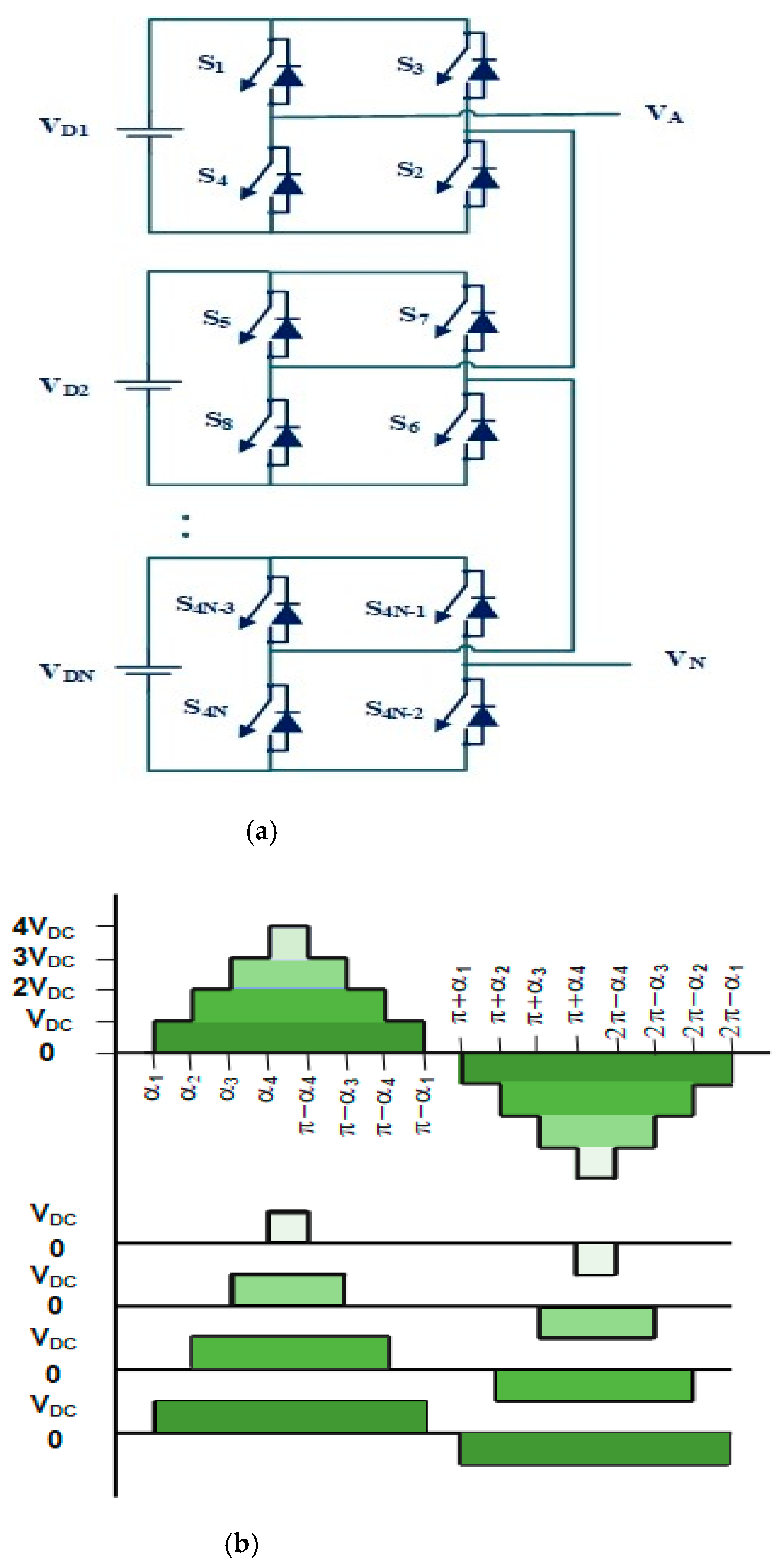
The most commonly used MLI is the Cascaded H Bridge Multilevel Inverter (CHB-MLI) as compared to the diode-clamped inverter and the flying capacitor inverter, since its structure is modular and simple. The number of levels in CHB-MLI is defined by (2s+1), where s is the number of single-phase full-bridge inverters. The output voltage of the CHB-MLI can be controlled by using either a high or low-frequency PWM technique. Implementing a high switching frequency technique on CHB-MLI leads to power loss due to the presence of multiple switching devices. Selective harmonic elimination pulse width modulation (SHEPWM) technique is a low-frequency modulation scheme that ensures the elimination of the particular undesired lower harmonics. The researchers viably use the SHEPWM technique to reduce a large number of lower-order unwanted harmonics. However, this method needs transcendental equations to solve. The sheer complexity of the equations requires fast algorithms to solve them.

The methods to solve the SHEPWM problem can be classified as (1) numerical methods (NMs) (2) algebraic methods (AMs), and (3) evolutionary algorithms (EAs).

One of the famous numerical techniques in NMs is Newton–Raphson (NR) [1]. It is used in the transcendental equation in which systematic results are absent. The numerical technique includes algorithms, for instance, sequential quadratic programming and gradient optimization. NR has not been utilized for equal and non-equal DC voltage sources in a cascaded multilevel SHEPWM inverter structure despite its advantages. The particular reason for this circumstance is that cascaded multilevel inverter has a long iteration time since it requires selection of initial angles, making it practically non-convergent. Thus, for high-level inverter, NR becomes computationally complicated. The calculation of optimized switching angle using the polynomial equation in AMs [2] utilizes Groebner bases and resultant theory. Although these methods are independent of initial guesses, they are not used in real time and in cascade MLI because they have high complexity due to large calculations.

In EAs, the genetic algorithm (GA) [3] and new meta-heuristic optimization algorithms are used. However, they are only applied to equal DC sources because they fail to find the result in some modulation index values. For equal DC sources, GA removes the harmonic elimination problem, but it is not applicable for unequal sources.

For selective harmonic elimination (SHE), the genetic algorithm [2,4,5,6] can also be used in MLI. However, in the case of asymmetrical MLI, GA is not useful. Bee algorithm (BA) is proposed in [4,7], having superiority over GA. However, BA is analytically complex over GA. In [8,9], generalized pattern search (GPS) algorithms are introduced, which are straight search algorithms. However, they can only be utilized for small areas for local refinement.

In [10], VSI-based induction motor drive is used, but it can only be used in local minima and cannot find a viable solution for large problems. For a feasible modulation index, a memetic algorithm (MA) [11,12,13] converges to the accurate result. However, when the number of switching angles increases, ample time is taken by MA to evaluate solutions. In [14,15,16,17], the particle swarm optimization (PSO) algorithm is suggested, in which a lower number of active switches are used in MLI. It requires less driver circuit for calculating the best solution. For high-voltage and high-power conversion applications, in order to reduce switching losses and device stress, the PSO-NR algorithm is used, as was the case in [18]. With this algorithm, an initial value of the switching angle is found. However, this method produces depletion in diversity.

In [19], the modified particle swarm optimization (MPSO) algorithm is used for harmonic reduction in three-phase hybrid cascaded multilevel inverter. However, this algorithm takes a large amount of time for computing results due to its high complexity. In a 7-level inverter, the optimized solutions are found out by using GA and PSO separately [14]. Calculated switching angles provide the initial estimate to NR for local refinement. PSO has an inclination to fall towards local minima, and thus less suitable initials are calculated than GA. For asymmetrical MLI, PSO is put forward for a low number of switching angles; it decreases the calculation burden to find the result in contrast with the resultant theory approach and iterative method [15]. A hybrid PSO–NR algorithm is used in [18]. Particles move towards a global best position in this method, which results in a rise of convergence speed; however, it intensifies the problem of local minima. For better convergence rate and reduced harmonic content, the mesh adaptive direct search (MADS) algorithm is a cross with the MPSO algorithm in [20]. In [16], the species seed technique-based PSO (S-PSO) is introduced. However, computational complexity is increased due to large iteration being required in the Euclidean distance method, thus providing a low convergence rate.

Many other EA algorithms such as grey wolf optimization [21], cuckoo search algorithm [22], whale optimization algorithm [23], and differential search algorithm [24] are also proposed. However, the algorithm [21,22,23,24] provides feeble examination capability since it has an issue to remain at local minima. Moreover, they are not able to find reasonable solutions with the rise of the switching angle. Differential evolution (DE) is discussed in [25]; the algorithm is adequate, but when it is applied to a large number of levels, its analytical cost increases. Moreover, as compared to PSO, it takes a longer amount of time.

In this work, a new metaheuristic optimization algorithm is proposed. The artificial jellyfish algorithm (AJFS) [26] is inspired by the behavior of jellyfish in the ocean. AJFS is an ameliorated algorithm used in SHEPWM for the removal of unsolicited harmonics. In this algorithm, jellyfish tend to find the global best position by moving towards the ocean current or in a swarm to obtain a large quantity of nutritious food. Finally, all the jellyfish gather at the location where a considerable quantity of food is available. AJFS algorithm is advantageous over all the above algorithms. Its features are discussed below:

• The new meta-heuristic optimization algorithms overcome all boundaries and provide the most optimum and accurate solution eliminating harmonics.
• It provides optimal switching angle because its dependency on initial guesses is very minimal and it can thus find a more accurate solution.
• It can deal with computational complexity and have a high convergence speed, which makes it reliable.

In this paper, use of the AJFS algorithm led to lower-order harmonics in five-, seven-, and nine-level inverters becoming removed. Comparison of DE, GA, and AJFS is also discussed. The advantage of AJFS over DE and GA was confirmed by comparing THD values for a range of modulation indexes.

In the Section 2, working of multiple level inverters is discussed. In the Section 3, AJFS and its working principle is comprehensively explained. In the Section 4, AJFS is implemented into the Harmonic problem of SHEPWM. In the Section 5, the experimental result is demonstrated, whereas in the Section 6, the conclusion and the application of SHEPWM are presented.

2. Multilevel Inverter

2.1. Cascaded H Bridge Multilevel Inverter (CHB-MLI)

The CHBMLI structure comprises two or more H-bridge circuits connected in series. For each H-bridge, an independent DC source is provided. The voltage generated by each circuit is synthesized and added to provide output voltage. The generalized structure of CHB-MLI is depicted in Figure 1a. For an inverter with a DC source or switching angle equal to S, levels of inverter L are given by Equation (1),

$$L=2S+1$$

(1)

A nine-level staircase output voltage waveform is shown in Figure 1b.

2.2. Selective Harmonic Elimination Pulse Width Modulation (SHEPWM)

In SHEPWM, there are four variables in the nine-level inverter, i.e., ${\alpha }_1,{\alpha }_2,{\alpha }_3, \mathrm{and} {\alpha }_4$. The staircase output phase voltage waveform of MLI is examined by using Fourier series expansion in Equation (2)

$$V\left(\omega t\right)={{\displaystyle \sum }}_{n=1}^{\infty }{V}_n\sin \left(n\omega t\right)$$

(2)

where $V_n$ is defined as amplitude of nth harmonic.

$$V_n=\{\begin{array}{c}\frac{4V_D}{n\pi }{\displaystyle {\displaystyle \sum }_{i=1}^S}{K}_i\cos \left(n{\alpha }_i\right)\mathrm{odd}\\ 0 \mathrm{even}\end{array}$$

(3)

Here, $V_D$ is the source voltage, and $K_i$ is the ratio of $V_{Di}$ and $V_D$. The odd quarter/wave symmetric behavior make switching angle value bounded between 0 to π$/2(0<{\alpha }_1<{\alpha }_2\dots \dots <{\alpha }_S\le \frac{\pi }{2})$ and $i=1,2,3\dots \dots \dots S$; here, S represents switching angle of each level. S − 1 harmonics are removed from S switching angle and the fundamental is assured. Further, S harmonics are removed from S $+1$ variables that include S switching angle $+$ a dc source.

Equations (4)–(7) become as follows:

$$m=\frac{1}{S}\left(\cos {\alpha }_1+\cos {\alpha }_2+\cos {\alpha }_3\dots \dots \dots +\cos {\alpha }_s\right)$$

(4)

$$(\cos 5{\alpha }_1+\cos 5{\alpha }_2+\cos 5{\alpha }_3\dots \dots \dots +\cos 5{\alpha }_s)=0$$

(5)

$$(\cos p{\alpha }_1+\cos p{\alpha }_2+\cos p{\alpha }_3\dots \dots \dots +\cos p{\alpha }_s)=0$$

(6)

$$(\cos q{\alpha }_1+\cos q{\alpha }_2+\cos q{\alpha }_3\dots \dots \dots +\cos q{\alpha }_s)=0$$

(7)

Here, q represents a sequence of harmonic order following p that requires the eradication from the output voltage waveform.

The main objective of the SHEPWM technique is to achieve switching angles in such a way that it will manage the fundamentals to the desired value and remove particular order harmonics. In this paper, fifth harmonic is eliminated in the five-level inverter. The fifth and seventh harmonics are eliminated in the seven-level inverter. The 5th, 7th, and 11th harmonics are eliminated in the nine-level inverter. In the three-phase system with equal loading in the line-to-line voltage, triplen harmonic is cancelled out in the line voltage; therefore, the third harmonic and its multiples are not taken into account.

For the nine-level inverter, optimized firing angles are acquired by using Equations (8)–(11).

$$V_1=\frac{4V_D}{\pi }(\cos {\alpha }_1+\cos {\alpha }_2+\cos {\alpha }_3+\cos {\alpha }_4)=0$$

(8)

$$V_5=\frac{4V_D}{5\pi }(\cos 5{\alpha }_1+\cos 5{\alpha }_2+\cos 5{\alpha }_3+\cos 5{\alpha }_4)=0$$

(9)

$$V_7=\frac{4V_D}{7\pi }(\cos 7{\alpha }_1+\cos 7{\alpha }_2+\cos 7{\alpha }_3+\cos 7{\alpha }_4)=0$$

(10)

$$V_{11}=\frac{4V_D}{11\pi }(\cos 11{\alpha }_1+\cos 11{\alpha }_2+\cos 11{\alpha }_3+\cos 11{\alpha }_4)=0$$

(11)

For the nine-level inverter, to eliminate the 5th, 7th, and 11th harmonics, $V_5, V_7, \mathrm{and} V_{11}$ are set to zero. The numerous switching angles are achieved in different modulation indexes (m), which are defined by Equation (12),

$$m=\frac{\pi V_{desired}}{4S{V}_D} 0<m\le 1$$

(12)

Thus, the above Equations (8)–(11) can be written as below in Equations (13)–(16):

$$m=\frac{1}{S}\left(\cos {\alpha }_1+\cos {\alpha }_2+\cos {\alpha }_3\right)$$

(13)

$$(\cos 5{\alpha }_1+\cos 5{\alpha }_2+\cos 5{\alpha }_3+\cos 5{\alpha }_4)=0$$

(14)

$$(\cos 7{\alpha }_1+\cos 7{\alpha }_2+\cos 7{\alpha }_3+\cos 7{\alpha }_4)=0$$

(15)

$$(\cos 11{\alpha }_1+\cos 11{\alpha }_2+\cos 11{\alpha }_3+\cos 11{\alpha }_4)=0$$

(16)

Elimination of Fifth harmonic in the Five-Level Inverter

For the five-level inverter, AJFS algorithm provides an optimized switching angle that eliminates fifth harmonics. Moreover, fundamental obtains its desired value. There are two switching angles in a five-level inverter which is obtained by using Equations (17) and (18).

$$m=\frac{1}{2} \left[\cos \left({\alpha }_1\right)+\cos \left({\alpha }_2\right)\right]$$

(17)

$$\left(\cos 5{\alpha }_1+\cos 5{\alpha }_2\right)=0$$

(18)

Elimination of Fifth and Seventh Harmonics in the Seven-Level Inverter

There are three H-bridge modules for the seven-level inverter. The goal is to eliminate fifth and seventh harmonics and to acquire the desired fundamental voltage.

$$m=\frac{1}{3} \left[\cos \left({\alpha }_1\right)+\cos \left({\alpha }_2\right)+\cos \left({\alpha }_3\right)\right]$$

(19)

$$\left(\cos 5{\alpha }_1+\cos 5{\alpha }_2+\cos 5{\alpha }_3\right)=0$$

(20)

$$\left(\cos 7{\alpha }_1+\cos 7{\alpha }_2+\cos 7{\alpha }_3\right)=0$$

(21)

3. AJFS Algorithm

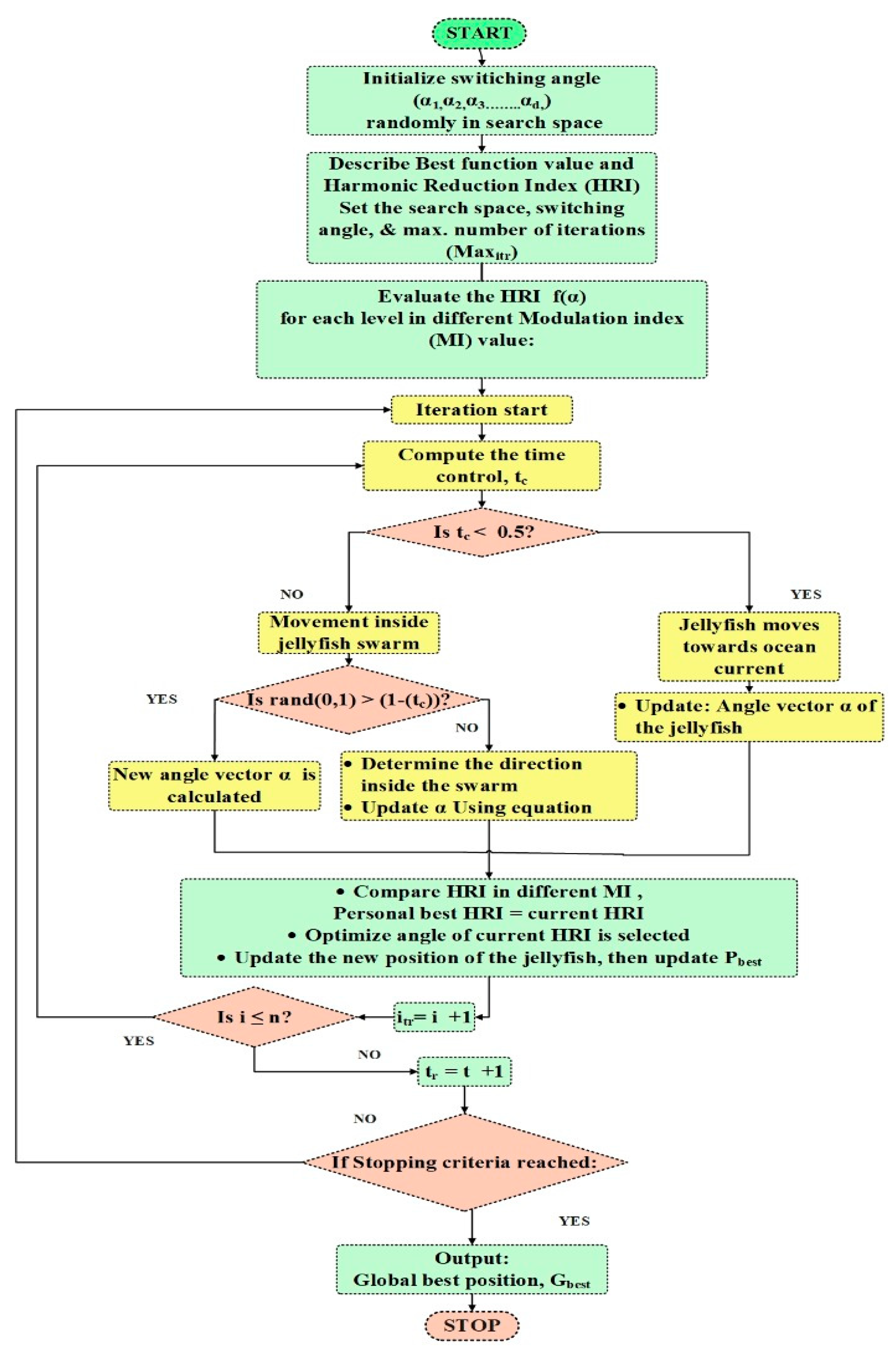
The artificial jellyfish search (AJFS) optimizer is a metaheuristic algorithm [27] inspired by a jellyfish’s performance in the ocean, as shown in Figure 2. The spark of a scrutinizing behavior of jellyfish includes their motion towards the ocean current or moving in the swarm (performing either active or passive movement). A time control technique is utilized for switching among these movements.

The artificial jellyfish search algorithm is based on three idealized procedures:

✓

In the ocean, jellyfish travel inside the swarm or follow the ocean current. In order to control the switching between the types of motion, a time control mechanism (t_c) is used.

✓

It is analyzed that jellyfish will get attracted to that location where the available quantity of food is high.

✓

The harmonic reduction index (HRI) calculates the particular location where a large quantity of food is present.

At the start, food is searched for by jellyfish in the ocean. The location where the available quantity of food is high attracts jellyfish to that position. The HRI manifests different sites where the jellyfish visited, wherein the quantity of food is present at that location. The proportion of food is compared and analyzed in each iteration and, finally, global best position is determined where the best and largest quantity of food is available.

The initialization position of jellyfish is $f\left(\alpha \right)$ and where the food is present in vast quantity is assumed to be the current best position $({\alpha }^{*})$. There are two motions performed by a jellyfish swarm, i.e., active or passive motion. Active motion is performed by jellyfish when the swarm is just established. After that, passive motion is performed. Movement of jellyfish around their own position is called active motion and its position associated with each location is updated in Equation (22).

$${\alpha }_L^{t+1}={\alpha }_L^t+rand\left(0,1\right)\times rand\left(0,1\right)\times \mu$$

(22)

where $\mu =$ mean location of all jellyfish. The other jellyfish M follows passive motion in contrast to jellyfish L, who follows active motion. Passive motion is performed in order to determine the position of motion by selecting a random position and vector from the jellyfish L. If the quantity of food at the jellyfish M location is greater than the quantity of food at jellyfish L location, L will move towards the M, and if L has more food than M, it will move away from its food location in order to determine the other best location. Hence, each jellyfish is able to obtain a large amount of food by moving in the appropriate direction. Thus, the way in which to find the global best position iteration is performed in various directions of motion, and the best position is updated.

$$Direction=\{\begin{array}{c}{\alpha }_M^t\left(t\right)-{\alpha }_L^M\left(t\right) if f\left({\alpha }_L\right)\ge f \left({\alpha }_M\right)\\ {\alpha }_L\left(t\right)-{\alpha }_M\left(t\right) if f\left({\alpha }_L\right)<f\left({\alpha }_M\right)\end{array}$$

(23)

where $f$ is the harmonic reduction index of location $\alpha$. For each successive iteration, the new position of jellyfish is given by Equation (24).

$${\alpha }_L^{t+1}={\alpha }_L^t+rand\left(0,1\right)\times Direction$$

(24)

The time control technique is utilized for analyzing the type of motion over time. It helps to govern active and passive motion and examine the motion of jellyfish if they are pointing towards an ocean current.

Constant C₀ and time control function $t_c$ are involved in time control technique. The time control function is defined as an arbitrary value that oscillates from 0 to 1. It consists of constant C₀, which is equal to 0.5 as it is the mean value of 0 and 1.

The time control function is a random value that fluctuates from 0 to 1 and is calculated in Equation (25).

$$t_c=\left|\left(1-\frac{t}{Ma{x}_{iter}}\right)\times \left(2\times rand\left(0,1\right)-1\right)\right|$$

(25)

where $t_c$ is the number of time-based iterations and $Ma{x}_{int}$ is the maximum number of iterations. Jellyfish move towards the position where a large amount of healthy food is available, leading to the formation of a swarm. Jellyfish inside the swarm move towards another ocean current, and another jellyfish swarm is generated due to the variation of time, which leads to change in temperature and wind direction.

If $t_c\ge 0.5$, jellyfish point towards ocean current. Ocean current is determined by Equation (26).

$$current={\alpha }^{*}-\beta \times rand\left(0,1\right)\times \mu$$

(26)

where $\beta =$ distribution coefficient, and $\mu =$ mean location of all jellyfish. If $rand\left(0,1\right)<\left(1-t_c\right)$, jellyfish start moving inside the swarm, wherein they follow the active or passive motion. Furthermore, when $rand\left(0,1\right)>\left(1-t_c\right)$, it exhibits passive motion, and if $rand\left(0,1\right)<\left(1-t_c\right)$, active motion is performed.

Increasing the convergence speed to high value and making the algorithm independent at local optima leads to the diversity of the initial population becoming ameliorated. The logistic map is used. This map provides negligible chances of premature convergence and helps to provide enormous divergence in the initial population.

The map equation is given by Equation (27).

$${\alpha }_{L+1}=4{\alpha }_L\left(1-{\alpha }_L\right),0\le {\alpha }_0\le 1$$

(27)

The end boundary condition is checked, and the quantity of food at the new location is calculated. On each iteration, the location of each jellyfish is updated and continues until it reaches to a $Ma{x}_{iter }$, and it is stopped when $t$ > $Ma{x}_{iter}$.

After that, global best position of jellyfish is obtained, wherein food $({\alpha }^{*})$ is available in large quantities. The working of AJFS algorithm has been explained using a flowchart in Figure 2.

4. Implementation of the Selective Harmonic Problem

The SHEPWM solution is inaccessible in a few areas of m that remove unsolicited harmonics. The implementation of the AJFS algorithm into the harmonic problem of SHEPWM is explained in Figure 3.

The optimized switching angles are calculated using the harmonic reduction index value as given in the Equation (28).

$$HRI=min\left[{\left|100\frac{V_{needed}-V_1}{V_{needed}}\right|}^4+{\displaystyle {\displaystyle \sum }_{i=2}^i}\frac{1}{h_i}{\left|50\frac{V_{h_i}}{V_1}\right|}^2\right]$$

(28)

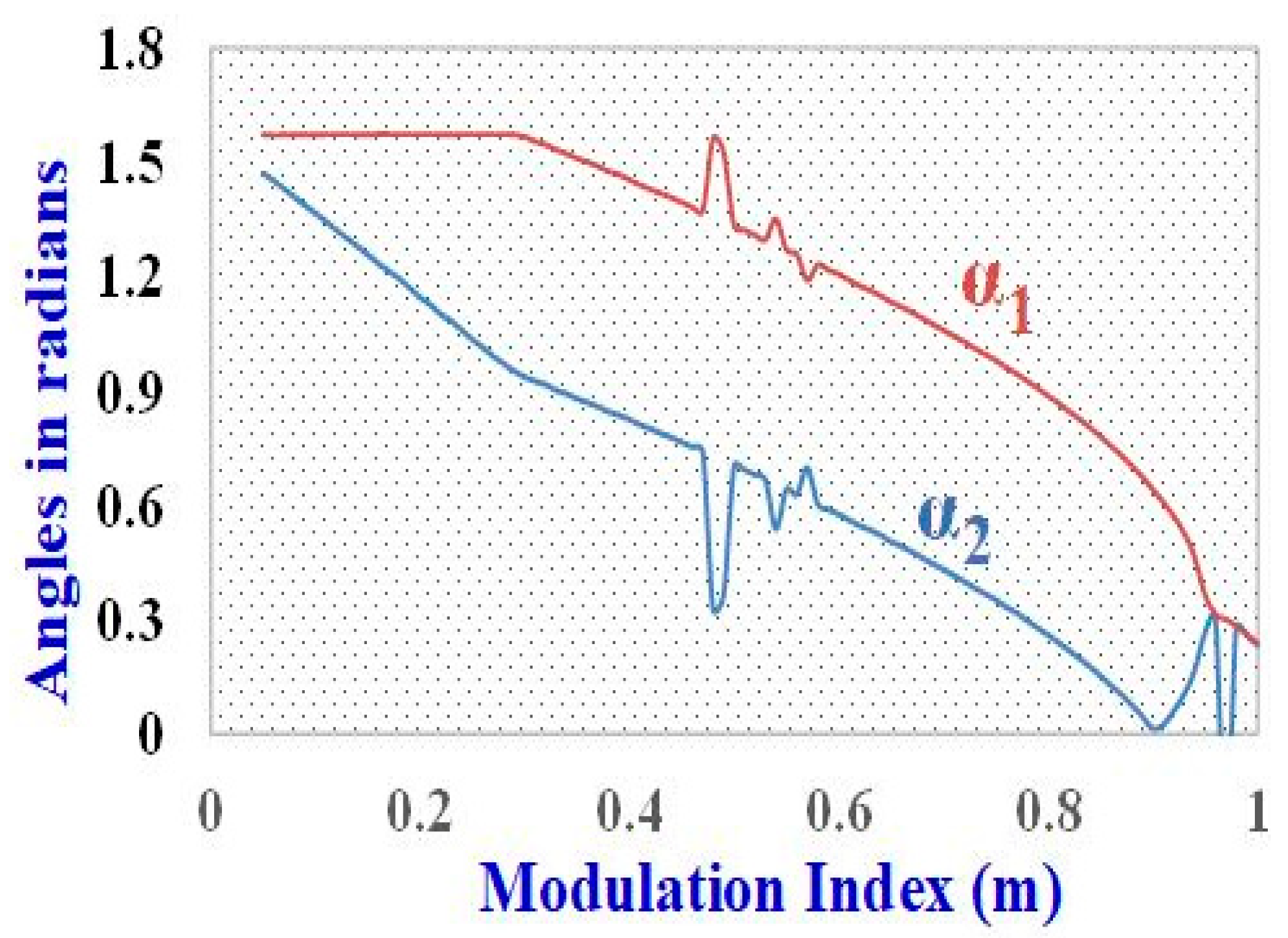
where $V_1$ is the fundamental voltage, $V_{needed}$ is the needed fundamental voltage, and $h_i$ is the order of harmonics (i.e., $h_2=3,h_3=5$, and so on). To obtain the needed fundamental voltage, the foremost part of HRI is excellent because of the power of 4 to retain the error among $V_1$ and $V_{needed}$ under 1%. If the error is less than 1%, there is a nugatory effect by the power. The later part of HRI is having square power to retain unwanted low-order harmonics under 2% error. Moreover, to significantly increase the elimination of specific harmonics, this part is divided by its harmonic order. For five-, seven-, and nine-level inverters, optimized switching angle is achieved through having unequal input DC sources for $0.05\le m\le 1$ with 0.01 step value. 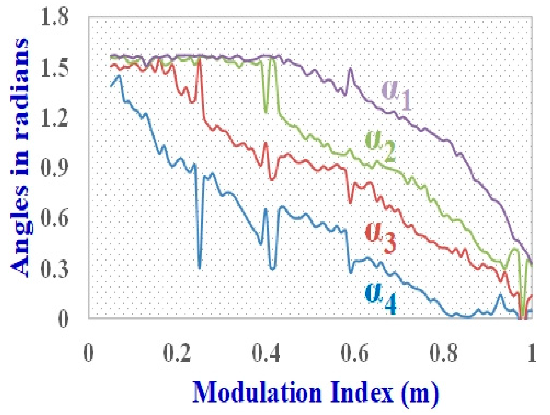In five-level inverters, $\left({\alpha }_1,{\alpha }_2\right)$ are computed; for seven-level inverters, $\left({\alpha }_1,{\alpha }_2,{\alpha }_3\right)$ are analyzed; and in the nine-level inverters, $({\alpha }_1,{\alpha }_2,{\alpha }_3,{\alpha }_4$) are evaluated for a range of m, which varies from 0.08 to 1, and distinct values of firing angle are calculated by writing the present algorithm in MATLAB, with the outcomes shown in Figure 4, Figure 5 and Figure 6, respectively.

The artificial jellyfish search (AJFS) reduces HRI to a compact value for five, seven, and nine levels, as shown in Figure 7. The precision of the result is manifest by a small value of the harmonic reduction index. The small value of HRI makes the value of lower-order harmonics near to zero.

The results of DE, GA, and AJFS were compared by plotting THD vs. m graph, as shown in Figure 8, Figure 9 and Figure 10 for five-, seven-, and nine-level inverters, respectively. By analyzing values at different ranges of m, we found that in the case of AJFS, the THD value was reduced more significantly than DE and GA. The lower value of THD claimed the superiority of the AJFS algorithm.

For the five-level inverter, the output waveform of voltage and current at m 0.69 and 0.93 with an RL (50 Ω + 800 mH) load is shown in Figure 11a. For the seven-level inverter, the output waveform of voltage and current having m 0.71 and 0.92 and RL (50 Ω + 800 mH) load is shown in Figure 11b. For the nine-level inverter, the output waveform of voltage and current at m 0.83 and 0.91 with an RL (50 Ω + 800 mH) load is shown in Figure 11c. Figure 11d–i depicts the output phase voltage FFT of five-level inverter at m 0.69 and 0.93, seven-level inverter at m 0.71 and 0.92, and nine-level inverter at m 0.83 and 0.91, respectively. The selected parameters which are used in AJFS algorithm are shown in

Table 1. Selected parameters in AJFS.

Symbol	Quantity
${\alpha }_1,{\alpha }_2,{\alpha }_3\dots \dots \dots {\alpha }_d$	initialize switching angle
$I_{tr\left(max\right)}$	maximum number of iterations
$t_c$	time control
$\beta$	distribution coefficient
$\mu$	mean location of all jellyfish
$\gamma >0$	movement coefficient
$c^t$	time control function
$Ma{x}_{int}$	maximum number of iterations
$U_b$	upper boundary of examine space
$L_b$	lower boundary of examine space
$P_{best}$	global best position

.

The five-level inverter’s respective initialization switching angle and harmonic reduction index with varying modulation index is represented in

Table 2. Firing angles and HRI for five-level inverter.

m	α1	α2	Harmonic Reduction Index
0.58	0.600765	1.228799	$1.46\times {10}^{-5}$
0.68	0.460008	1.088594	$2.67\times {10}^{-4}$
0.81	0.238032	0.866379	$5.33\times {10}^{-6}$
0.94	0.163763	0.464611	$7.04\times {10}^{-6}$

.

There are two h-bridges in the five-level inverter in order to eliminate the fifth-order harmonic; two switching angles are optimized, and the desired value of the fundamental harmonic is also achieved. In the Figure 11d,e, the fifth harmonic is eliminated in m 0.69 and 0.93, and the simulation is performed for various m ranges from 0.3 to 1 with a step of 0.01.

In the seven-level inverter, the main objective is to remove the fifth and seventh harmonics. Modulation index (m) varies from 0.3 to 1. Three optimum switching angles are chosen ${\alpha }_1,{\alpha }_2, \mathrm{and} {\alpha }_3.$ The fifth and seventh harmonics are completely eliminated and the desired value of fundamental is achieved, as shown in Figure 11f,g, with its corresponding voltage and the current waveform being shown in Figure 11b.

In nine-level CHB-MLI, two DC sources are used, having values of 30 V and 90 V, and four optimum switching angles are chosen as ${\alpha }_1,{\alpha }_2,{\alpha }_3, \mathrm{and} {\alpha }_4$ for different MI to eliminate 5th, 7th, and 11th harmonics. The waveforms at m 0.83 and 0.91 are shown in Figure 11c, and their associated voltage FFT analysis is shown in Figure 11h,i. The 5th, 7th, and 11th harmonics are completely removed. For nine-level, MI varies from 0.3 to 1. The low value of THD validates the efficacy of AJFS algorithm. For a lower value of m, the output waveform has low amplitude compared to the larger value of m. The more the sinusoidal output current waveform, the smaller the harmonics present. Moreover, the desired output is achieved at each level. The output voltage waveform changes as per the value of the firing angle and the input DC voltage. In the fifth level inverter, fundamental values of the output voltage were 99.35 V and 240 V at m of 0. 69 and 0.93, respectively. In the case of the seventh level, the observed fundamental output voltage had values 108.8 V and 110.4 V at m 0.71 and 0.92, respectively. For the ninth level inverter at m 0.83, the fundamental voltage was 126.8 V, and at m 0.91, the fundamental voltage was 139.7 V. The desired amplitude of the fundamental was obtained at the output and, consequently, the output power was also achieved.

5. Experimental Results

The simulation results are being confirmed experimentally for three phase five, seven and nine level inverter. The experiment setup organized to achieve the particular result are shown in Figure 12.

In the development of CHB-MLI, the IGBT (IGB20N60H3) is utilized. The DC was supplied in different levels of the inverter as follows: for five-level, it was 60 V in both VDC1 and VDC2; in seven-level, it was 40 V in VDC1 and 80 V in VDC2; for the nine-level, it was 90 V in VDC1 and 30 V in VDC2. AJFS was used to find optimized switching angles in each m for a different level of MLI. The calculated value of the optimized switching angle (${\alpha }_1,{\alpha }_2,{\alpha }_3\dots \dots {\alpha }_s$) of each level was stored in a lookup table.

Value from the lookup table was given to the digital signal controller board (TMS320F28379) to generate the pulse pattern of the SHEPWM signal. The coming signal from the digital signal controller board was transferred to the TLP 250-based IC driver board that was applied to control the given signal. Tektronix TDS 2024B oscilloscope was utilized for showing output waveforms and for computing THD.

For different MI, the experiment was executed, which is elaborated in Table 2. The outcomes for different levels of the inverter are depicted in Figure 13, which are carried out in different loads and conditions. The output phase voltage measured for five-level inverter at m 0.63 and RL (50 Ω + 800 mH) load and manifested in Figure 13a alongside with its correlated harmonic spectrum. The fifth harmonic was completely eliminated. The peak voltage was 142 V. The RMS voltage and current were 38.4 V and 1.25 A, respectively. In the case of fifth level, the 3rd, 7th, 9th, and 11th harmonics were 5%, 2%, 4% and 3% of fundamental respectively and 5th harmonics were completely eliminated. The output phase voltage measured for seven-level inverter at m 0.79 with RL (50 Ω + 800 mH) load shown in Figure 13b, alongside its associated harmonic spectrum. The fifth and seventh harmonics were removed. The peak voltage was 154 V, and the RMS voltage was found to be 49.1 V. In the case of the seventh level, the 3rd, 9th, 11th, and 13th were 4%, 3%, 2%, and 3.5% of fundamental, respectively. The desired output power was achieved. 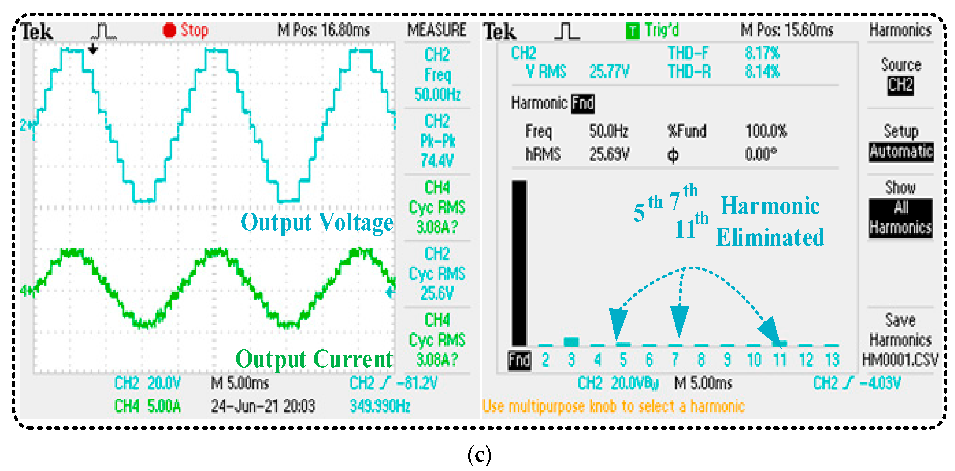Figure 13c shows the output phase voltage for nine-level measured at m 0.71 with RL (50 Ω + 800 mH) load, and their related harmonic spectrum is also shown in same figure. The 5th, 7th, and 11th harmonics were eliminated with considerably low value of THD and with a peak voltage equal to 74.4 V; the RMS voltage and were current found to be 25.6 V and 3.08 A, respectively.

6. Conclusions

In this paper, lower-order harmonics were considerably eliminated, and the desired output voltage was achieved using the SHEPWM technique. A novel search algorithm AJFS was used to obtain switching angles for a different level of the inverter, and it was found to be convenient for CHB-MLI by removing undesired lower-order harmonics. The proposed algorithm for Cascaded H Bridge multilevel inverter was applied in heat control of electric drive system and bridge connection of solar PV system. Moreover, it was utilized in induction motors and was also used in grid connection in the distributed generation system. Figure 14 shows the application of SHEPWM in the standalone PV system. For a five-level inverter, it removes fifth order harmonics. For a seven-level inverter, it removes fifth and seventh order harmonics. Moreover, in a nine-level inverter, it eliminates 5th, 7th, and 11th order harmonics. The range of $m$ confirms that AJFS can provide a lower value of THD as compared to DE and GA. The algorithm overcomes many limitations because it has a high convergence speed, provides high divergence in the initial population, reduces switching losses, and eliminates lower-order harmonics. The accurate solution is achieved, and computational complexity decreases, which was validated by simulation and experimental results.