
Cooperative- and Eco-Driving: Impact on Fuel Consumption for Heavy Trucks on Hills


Abstract
: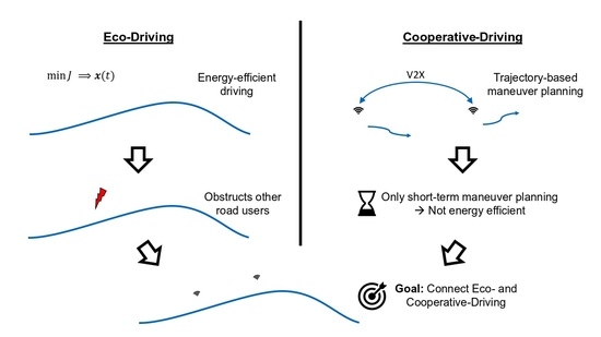
1. Introduction
2. Related Work
2.1. Eco-Driving
2.2. Cooperative Driving
2.3. Vehicle-to-Everything Communication
2.4. Summary
3. Method
| Algorithm 1 Definition of MCM in the Protocol Buffers notation. |
| syntax = “proto3”; |
| message MCM { |
| uint32 v2xId = 1;//V2X station ID |
| int64 timestamp = 2;//time in us |
| Trajectory planTra = 3;//planed trajectory |
| optional Trajectory desireTra = 4;//desired trajectory |
| message Trajectory { |
| repeated PolySection longPos = 1;//UTM-easting |
| repeated PolySection latPos = 2;//UTM-northing |
| message PolySection { |
| repeated float coefficients = 1;//coefficients of polynomial a_0, a_1, … |
| float start = 2;//start time in s, real start time = start time + timestamp |
| float end = 3;//end time in s, real end time = start time + timestamp |
| float xOffset = 4;//UTM-Offset, whole number because of accuracy float32 |
| } |
| } |
| } |
- Stage 1: Safety distance according to StVO + double tolerances of the trajectory.
- Stage 2: Safety distance according to StVO in first, e.g., three seconds, otherwise like Stage 1.
- Stage 3: Safety distance according to StVO.
4. Evaluation
4.1. Simulation Environment
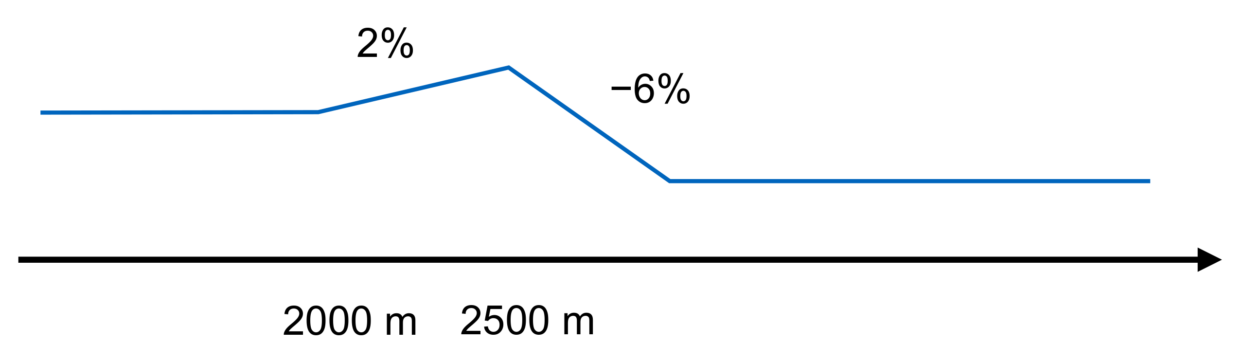
4.2. Scenarios
4.3. Results
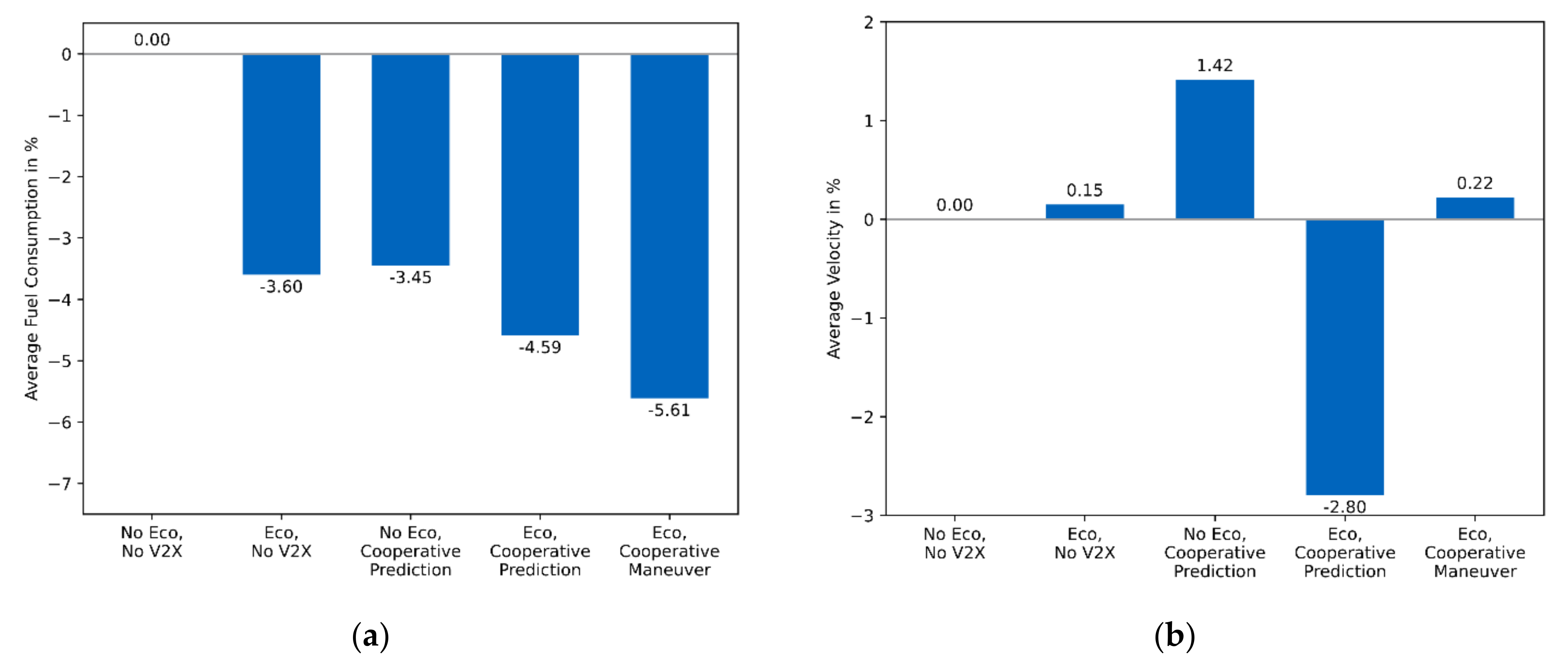
4.3.1. Two Trucks
4.3.2. Three Trucks
5. Discussion
6. Conclusions
Author Contributions
Funding
Data Availability Statement
Acknowledgments
Conflicts of Interest
References
- Bundesministerium für Umwelt, Naturschutz und Nukleare Sicherheit. Klimaschutz in Zahlen: Fakten, Trends und Impulse Deutscher Klimapolitik. Available online: https://www.bmu.de/fileadmin/Daten_BMU/Pools/Broschueren/klimaschutz_zahlen_2019_broschuere_bf.pdf (accessed on 17 February 2021).
- Bunz, M.; Mücke, H.-G. Klimawandel—physische und psychische Folgen. Bundesgesundh. Gesundh. Gesundh. 2017, 60, 632–639. [Google Scholar] [CrossRef] [PubMed]
- Masson-Delmotte, V. Global Warming of 1.5 °C: An IPCC Special Report on the Impacts of Global Warming of 1.5 °C Above Pre-Industrial Levels and Related Global Greenhouse Gas Emission Pathways, in the Context of Strengthening the Global Response to the Threat of Climate Change, Sustainable Development, and Efforts to Eradicate Poverty. Available online: https://www.ipcc.ch/sr15/ (accessed on 17 February 2021).
- European Commission. The European Green Deal. Available online: https://eur-lex.europa.eu/legal-content/DE/TXT/?qid=1576150542719&uri=COM%3A2019%3A640%3AFIN (accessed on 15 September 2021).
- Nowak, G.; Maluck, J.; Stürmer, C.; Pasemann, J. The Era of Digitized Trucking: Transforming the Logistics Value Chain. Available online: https://www.strategyand.pwc.com/media/file/The-era-of-digitized-trucking.pdf (accessed on 23 June 2019).
- Esch, T.; Dahlhaus, U. Antrieb. In Nutzfahrzeugtechnik: Grundlagen, Systeme, Komponenten, 8; Überarbeitete und Erweiterte Auflage, Hoepke, E., Breuer, S., Eds.; Springer Vieweg: Wiesbaden, Germany, 2016; pp. 403–540. ISBN 978-3-658-09537-6. [Google Scholar]
- Walnum, H.J.; Simonsen, M. Does driving behavior matter? An analysis of fuel consumption data from heavy-duty trucks. Transp. Res. Part D Transp. Environ. 2015, 36, 107–120. [Google Scholar] [CrossRef]
- Zhou, M.; Jin, H.; Wang, W. A review of vehicle fuel consumption models to evaluate eco-driving and eco-routing. Transp. Res. Part D Transp. Environ. 2016, 49, 203–218. [Google Scholar] [CrossRef]
- International Council on Clean Transportation. Truck Eco-Driving Programs: Current Status in Latin America and International Best Practicies. Available online: https://theicct.org/sites/default/files/publications/eco-driving-latam-EN-apr2021.pdf (accessed on 13 September 2021).
- Huang, Y.; Ng, E.C.; Zhou, J.L.; Surawski, N.C.; Chan, E.F.; Hong, G. Eco-driving technology for sustainable road transport: A review. Renew. Sustain. Energy Rev. 2018, 93, 596–609. [Google Scholar] [CrossRef]
- Zavalko, A. Applying energy approach in the evaluation of eco-driving skill and eco-driving training of truck drivers. Transp. Res. Part D Transp. Environ. 2018, 62, 672–684. [Google Scholar] [CrossRef]
- MAN Truck & Bus, A.G. MAN EfficientCruise®—GPS-Gesteuerter Tempomat|MAN Lkw. Available online: https://www.truck.man.eu/de/de/man-welt/technologie-und-kompetenz/effizienzsysteme/gps-gestuetzter-tempomat/GPS-gestuetzter-Tempomat.html (accessed on 23 August 2017).
- Daimler, A.G. Predictive Powertrain Control—Schlauer Tempomat Spart Sprit. Available online: http://media.daimler.com/marsMediaSite/de/instance/ko/Predictive-Powertrain-Control---Schlauer-Tempomat-spart-Sprit.xhtml?oid=9917205 (accessed on 29 March 2018).
- Nordström, P.-E. Spectacular Fuel Savings—Scania Opticruise with Performance Modes. Available online: https://www.scania.com/group/en/spectacular-fuel-savings-scania-opticruise-with-performance-modes/ (accessed on 30 March 2018).
- Pudenz, K. Bei Steigung und Gefälle: I-See von Volvo Trucks Hilft Beim Kraftstoffsparen. Available online: https://www.springerprofessional.de/automobil---motoren/fahrerassistenz/bei-steigung-und-gefaelle-i-see-von-volvo-trucks-hilft-beim-kraf/6578176?searchResult=1.bei%20steigung%20gef%C3%A4lle%20i%20see%20von%20volvo%20trucks%20hilft&searchBackButton=true (accessed on 29 March 2018).
- Renault Trucks. Optivision. Available online: http://www.renault-trucks.de/aktuelles/optivision-k4z.html (accessed on 30 March 2018).
- DAF Trucks, N.V. Predictive Cruise Control. Available online: http://www.daftrucks.de/de-de/trucks/comfort-and-safety-systems-euro-6/predictive-cruise-control (accessed on 30 March 2018).
- Iveco Magirus, A.G. Der neue STRALIS: TCO2 Champion. Available online: https://www.iveco.com/austria/neufahrzeuge/pages/tco2-champion-stralis-truck-aspx.aspx (accessed on 3 March 2018).
- Sciarretta, A.; Vahidi, A. Energy-Efficient Driving of Road Vehicles; Springer International Publishing: Cham, Switzerland, 2020; ISBN 978-3-030-24126-1. [Google Scholar]
- Hellström, E. Look-Ahead Control of Heavy Vehicles; Department of Electrical Engineering, Linköping University: Linköping, Switzerland, 2010; ISBN 978-91-7393-389-6. [Google Scholar]
- Fafoutellis, P.; Mantouka, E.G.; Vlahogianni, E.I. Eco-Driving and Its Impacts on Fuel Efficiency: An Overview of Technologies and Data-Driven Methods. Sustainability 2021, 13, 226. [Google Scholar] [CrossRef]
- Saerens, B. Optimal Control Based Eco-Driving: Theoretical Approach and Practical Applications. Ph.D. Thesis, Katholieke Universiteit Leuven, Heverlee, Belgium, 2012. [Google Scholar]
- Roth, M.; Radke, T.; Lederer, M.; Gauterin, F.; Frey, M.; Steinbrecher, C.; Schröter, J.; Goslar, M. Porsche InnoDrive—An Innovative Approach for the Future of Driving. In Proceedings of the 20th Aachen Colloquium Automobile and Engine Technology, Aachen, Germany, 10 October–12 November 2011; pp. 1453–1467. [Google Scholar]
- BMW, A.G. Efficient Driving: Lower Consumption and Increase Range with BWM Efficient Dynamics. Available online: https://www.bmw.cc/en/topics/fascination-bmw/efficient-dynamics/energy-management.html (accessed on 5 August 2021).
- Audi, A.G. Driver Assistance Systems. Available online: https://www.audi-mediacenter.com/en/technology-lexicon-7180/driver-assistance-systems-7184 (accessed on 5 August 2021).
- Samaras, Z.; Ntziachristos, L.; Toffolo, S.; Magra, G.; Garcia-Castro, A.; Valdes, C.; Vock, C.; Maier, W. Quantification of the Effect of ITS on CO2 Emissions from Road Transportation. Transp. Res. Procedia 2016, 14, 3139–3148. [Google Scholar] [CrossRef] [Green Version]
- Alam, A. Fuel-Efficient Heavy-Duty Vehicle Platooning. Ph.D. Thesis, KTH Royal Institute of Technology, Stockholm, Sweden, 2014. [Google Scholar]
- Ulbrich, S.; Grossjohann, S.; Appelt, C.; Homeier, K.; Rieken, J.; Maurer, M. Structuring Cooperative Behavior Planning Implementations for Automated Driving. In Proceedings of the 2015 IEEE 18th International Conference on Intelligent Transportation Systems (ITSC 2015), Gran Canaria, Spain, 15–18 September 2015; IEEE: Piscataway, NJ, USA, 2015; pp. 2159–2165, ISBN 978-1-4673-6596-3. [Google Scholar]
- Eiermann, L.; Sawade, O.; Bunk, S.; Breuel, G.; Radusch, I. Cooperative automated lane merge with role-based negotiation. In Proceedings of the 2020 IEEE Intelligent Vehicles Symposium (IV), Las Vegas, NV, USA, 20–23 October 2020. [Google Scholar]
- Lehmann, B.; Gunther, H.-J.; Wolf, L. A Generic Approach towards Maneuver Coordination for Automated Vehicles. In Proceedings of the 2018 21st International Conference on Intelligent Transportation Systems (ITSC), Maui, HI, USA, 4–7 November 2018; IEEE: Piscataway, NJ, USA, 2018; pp. 3333–3339, ISBN 978-1-7281-0322-8. [Google Scholar]
- Llatser, I.; Michalke, T.; Dolgov, M.; Wildschuette, F.; Fuchs, H. Cooperative Automated Driving Use Cases for 5G V2X Communication. In Proceedings of the 2019 IEEE 2nd 5G World Forum (5GWF), Dresden, Germany, 30 September–2 October 2019; pp. 120–125. [Google Scholar]
- Tami, R.; Soualmi, B.; Doufene, A.; Ibanez, J.; Dauwels, J. Machine learning method to ensure robust decision-making of AVs. In Proceedings of the 2019 IEEE Intelligent Transportation Systems Conference (ITSC), Auckland, New Zealand, 27–30 October 2019; IEEE: Piscataway, NJ, USA, 2019; pp. 1217–1222, ISBN 978-1-5386-7023-1. [Google Scholar]
- Hauenstein, J.; Diermeyer, F. Cooperative Longitudinal Control for Commercial Vehicles. In 9. Tagung Automatisiertes Fahren. 9; Tagung Automatisiertes Fahren: Munich, Germany, 2019. [Google Scholar]
- Sciarretta, A.; Nunzio, G.D.; Ojeda, L.L. Optimal Ecodriving Control: Energy-Efficient Driving of Road Vehicles as an Optimal Control Problem. IEEE Control Syst. 2015, 35, 71–90. [Google Scholar] [CrossRef] [Green Version]
- Radke, T. Energieoptimale Längsführung von Kraftfahrzeugen Durch Einsatz Vorausschauender Fahrstrategien; Karlsruher Institut für Technologie: Karlsruhe, Germany, 2013. [Google Scholar]
- Haken, K.-L. Grundlagen der Kraftfahrzeugtechnik, 2., Akualisierte und Erw. Aufl.; Hanser: München, Germany, 2011; ISBN 978-3-446-42849-2. [Google Scholar]
- Ayoubi, M.; Eilemann, A.; Mankau, H.; Pantow, E.; Repmann, C.; Seiffert, U.; Wawzyniak, M.; Wiebelt, A. Fahrzeugphysik. In Vieweg Handbuch Kraftfahrzeugtechnik; Pischinger, S., Seiffert, U., Eds.; Springer: Wiesbaden, Germany, 2016; pp. 57–130. ISBN 978-3-658-09527-7. [Google Scholar]
- Breuer, S.; Kopp, S. Fahrmechanik. In Nutzfahrzeugtechnik: Grundlagen, Systeme, Komponenten, 8; Überarbeitete und Erweiterte Auflage, Hoepke, E., Breuer, S., Eds.; Springer Vieweg: Wiesbaden, Germany, 2016; pp. 37–122. ISBN 978-3-658-09537-6. [Google Scholar]
- Grundgedanken, G. Straßenverkehrs-Ordnung (StVO). Available online: https://www.gesetze-im-internet.de/stvo_2013/ (accessed on 21 July 2018).
- Khalik, Z.; Padilla, G.P.; Romijn, T.; Donkers, M. Vehicle Energy Management with Ecodriving: A Sequential Quadratic Programming Approach with Dual Decomposition. In Proceedings of the 2018 Annual American Control Conference (ACC), Milwaukee, WI, USA, 27–29 June 2018; pp. 4002–4007, ISBN 978-1-5386-5428-6. [Google Scholar]
- Bauer, K.-L. Echtzeit-Strategieplanung für Vorausschauendes Automatisiertes Fahren; Karlsruher Institut für Technologie: Karlsruhe, Germany, 2019. [Google Scholar]
- Huber, M. Verfahren zum Betreiben Eines Fahrzeuges, Insbesondere Eines Nutzfahrzeuges, Steuer- und/oder Auswerteeinrichtung, Fahrerassistenzsystem für ein Nutzfahrzeug Sowie Nutzfahrzeug. DE102008023135B4, 12 November 2009. [Google Scholar]
- Düring, M.; Pascheka, P. Cooperative decentralized decision making for conflict resolution among autonomous agents. In Proceedings of the 2014 IEEE International Symposium on Innovations in Intelligent Systems and Applications (INISTA), Alberobello, Italy, 23–25 June 2014; IEEE: Piscataway, NJ, USA, 2014; pp. 154–161, ISBN 978-1-4799-3020-3. [Google Scholar]
- Burger, C.; Orzechowski, P.F.; Tas, O.S.; Stiller, C. Rating cooperative driving: A scheme for behavior assessment. In Proceedings of the IEEE ITSC 2017, 20th International Conference on Intelligent Transportation Systems: Mielparque Yokohama in Yokohama, Kanagawa, Japan, 16–19 October 2017; IEEE: Piscataway, NJ, USA, 2017; pp. 1–6, ISBN 978-1-5386-1526-3. [Google Scholar]
- Okoso, A.; Otaki, K.; Nishi, T. Multi-Agent Path Finding with Priority for Cooperative Automated Valet Parking. In Proceedings of the IEEE ITSC 2019, 2019 22st International Conference on Intelligent Transportation Systems (ITSC) Auckland, New Zealand, 27–30 October 2019; IEEE: Piscataway, NJ, USA, 2019; pp. 2135–2140, ISBN 978-1-5386-7023-1. [Google Scholar]
- Knies, C.; Hermansdorfer, L.; Diermeyer, F. Cooperative Maneuver Planning for Highway Traffic Scenarios based on Monte-Carlo Tree Search. AAET Automatisiertes und Vernetztes Fahren: Beiträge zum gleichnamigen 20. Braunschweiger Symposium am 6. und 7. Februar 2019, Stadthalle, Braunschweig, 1. Auflage; ITS mobility e.V: Braunschweig, Germany, 2019; pp. 10–25. ISBN 978-3-937655-46-8. [Google Scholar]
- Sawade, O.; Schulze, M.; Radusch, I. Robust Communication for Cooperative Driving Maneuvers. IEEE Intell. Transport. Syst. Mag. 2018, 10, 159–169. [Google Scholar] [CrossRef]
- Heß, D.; Lattarulo, R.; Pérez, J.; Schindler, J.; Hesse, T.; Köster, F. Fast Maneuver Planning for Cooperative Automated Vehicles. In Proceedings of the IEEE ITSC 2018, 2018 21st International Conference on Intelligent Transportation Systems (ITSC), Maui, HI, USA, 4–7 November 2018; IEEE: Piscataway, NJ, USA, 2018; pp. 1625–1632, ISBN 978-1-7281-0322-8. [Google Scholar]
- Heß, D.; Lattarulo, R.; Perez, J.; Hesse, T.; Köster, F. Negotiation of Cooperative Maneuvers for Automated Vehicles: Experimental Results. In Proceedings of the IEEE ITSC 2019, 2019 22st International Conference on Intelligent Transportation Systems (ITSC), Auckland, New Zealand, 27–30 October 2019; IEEE: Piscataway, NJ, USA, 2019; pp. 1545–1551, ISBN 978-1-5386-7023-1. [Google Scholar]
- Festag, A. Standards for vehicular communication—From IEEE 802.11p to 5G. Elektrotech. Inftech. 2015, 132, 409–416. [Google Scholar] [CrossRef]
- Weber, R.; Misener, J.; Park, V. C-V2X—A Communication Technology for Cooperative, Connected and Automated Mobility. In Proceedings of the Mobile Communication Technologies and Applications; 24. ITG-Symposium, Osnabrueck, Germany, 15–16 May 2019; pp. 111–116, ISBN 3800749610. [Google Scholar]
- Molina-Masegosa, R.; Gozalvez, J.; Sepulcre, M. Comparison of IEEE 802.11p and LTE-V2X: An Evaluation with Periodic and Aperiodic Messages of Constant and Variable Size. IEEE Access. 2020, 8, 121526–121548. [Google Scholar] [CrossRef]
- Naik, G.; Choudhury, B.; Park, J.-M. IEEE 802.11bd & 5G NR V2X: Evolution of Radio Access Technologies for V2X Communications. IEEE Access 2019, 7, 70169–70184. [Google Scholar] [CrossRef]
- Almeida, T.T.; de Gomes, C.L.; Ortiz, F.M.; Junior, J.G.R.; Costa, L.H.M.K. IEEE 802.11p Performance Evaluation: Simulations vs. Real Experiments. In Proceedings of the IEEE ITSC 2018, 2018 21st International Conference on Intelligent Transportation Systems (ITSC), Maui, HI, USA, 4–7 November 2018; IEEE: Piscataway, NJ, USA, 2018; pp. 3840–3845, ISBN 978-1-7281-0322-8. [Google Scholar]
- European Telecommunications Standards Institute. Intelligent Transport Systems (ITS); Decentralized Congestion Control Mechanisms for Intelligent Transport Systems Operating in the 5 GHz Range; Access Layer Part, V1.2.1, 2018 (ETSI TS 102 687). Available online: https://www.etsi.org/deliver/etsi_ts/102600_102699/102687/01.02.01_60/ts_102687v010201p.pdf (accessed on 30 July 2021).
- Eckhoff, D.; Sofra, N.; German, R. A performance study of cooperative awareness in ETSI ITS G5 and IEEE WAVE. In Proceedings of the 2013 10th Annual Conference on Wireless On-Demand Network Systems and Services (WONS 2013), Banff, AB, Canada, 18–20 March 2013; IEEE: Piscataway, NJ, USA, 2013; pp. 196–200, ISBN 978-1-4799-0749-6. [Google Scholar]
- Molina-Masegosa, R.; Gozalvez, J. LTE-V for Sidelink 5G V2X Vehicular Communications: A New 5G Technology for Short-Range Vehicle-to-Everything Communications. IEEE Veh. Technol. Mag. 2017, 12, 30–39. [Google Scholar] [CrossRef]
- Dey, K.C.; Rayamajhi, A.; Chowdhury, M.; Bhavsar, P.; Martin, J. Vehicle-to-vehicle (V2V) and vehicle-to-infrastructure (V2I) communication in a heterogeneous wireless network—Performance evaluation. Transp. Res. Part C Emerg. Technol. 2016, 68, 168–184. [Google Scholar] [CrossRef] [Green Version]
- Ganesan, K.; Lohr, J.; Mallick, P.B.; Kunz, A.; Kuchibhotla, R. NR Sidelink Design Overview for Advanced V2X Service. IEEE Internet. Things M 2020, 3, 26–30. [Google Scholar] [CrossRef]
- Rudschies, W. C2X im VW Golf 8: Erster ADAC Test. Available online: https://www.adac.de/rund-ums-fahrzeug/tests/assistenzsysteme/c2x-im-vw-golf-8/ (accessed on 5 October 2020).
- European Telecommunications Standards Institute. Intelligent Transport Systems (ITS); Security; Security Header and Certificate Formats, V1.4.1, 2020 (ETSI TS 103 097). Available online: https://www.etsi.org/deliver/etsi_ts/103000_103099/103097/01.04.01_60/ts_103097v010401p.pdf (accessed on 24 November 2020).
- European Telecommunications Standards Institute. Intelligent Transport Systems (ITS); Vehicular Communications; Basic Set of Applications; Part 2: Specification of Cooperative Awareness Basic Service, V1.3.2, 2014 (ETSI EN 302 637-2). Available online: http://www.etsi.org (accessed on 16 September 2018).
- European Telecommunications Standards Institute. Intelligent Transport Systems (ITS); Vehicular Communications; Basic Set of Applications; Part 3: Specifications of Decentralized Environmental Notification Basic Service, V1.2.2, 2014 (ETSI EN 302 637-3). Available online: http://www.etsi.org (accessed on 16 September 2018).
- European Telecommunications Standards Institute. Work Programme: Details of ‘DTS/ITS-00184’ Work Item. Available online: https://portal.etsi.org/webapp/WorkProgram/Report_WorkItem.asp?WKI_ID=53496&curItemNr=1&totalNrItems=1&optDisplay=10&qSORT=HIGHVERSION&qETSI_ALL=&SearchPage=TRUE&qETSI_NUMBER=103+561&qINCLUDE_SUB_TB=True&qINCLUDE_MOVED_ON=&qSTOP_FLG=&qKEYWORD_BOOLEAN=&qCLUSTER_BOOLEAN=&qFREQUENCIES_BOOLEAN=&qSTOPPING_OUTDATED=&butSimple=Search&includeNonActiveTB=FALSE&includeSubProjectCode=&qREPORT_TYPE=SUMMARY (accessed on 4 November 2020).
- Google LLC. Protocol Buffers. Available online: https://developers.google.com/protocol-buffers (accessed on 5 August 2021).
- European Telecommunications Standards Institute. Intelligent Transport Systems (ITS); Users and Applications Requirements; Part 2: Applications and Facilities Layer Common Data Dictionary, V1.2.1, 2014 (ETSI TS 102 894-2). Available online: https://www.etsi.org/deliver/etsi_ts/102800_102899/10289402/01.02.01_60/ts_10289402v010201p.pdf (accessed on 30 July 2021).
- Schubert, R.; Richter, E.; Wanielik, G. Comparison and evaluation of advanced motion models for vehicle tracking. In Proceedings of the 2008 IEEE 11th International Conference on Information Fusion, Cologne, Germany, 30 January–3 July 2008; IEEE: Piscataway, NJ, USA, 2008; pp. 730–735, ISBN 9783000248832. [Google Scholar]
- Hauenstein, J.; Gromer, J.; Mertens, J.C.; Diermeyer, F.; Kraus, S. Collective Perception: Impact on Fuel Consumption for Heavy Trucks. In Proceedings of the VEHITS 2021—7th International Conference on Vehicle Technology and Intelligent Transport Systems, Online Streaming, 28–30 April 2021; pp. 350–361, ISBN 978-989-758-513-5. [Google Scholar]
- Gonzalez, D.; Perez, J.; Milanes, V.; Nashashibi, F. A Review of Motion Planning Techniques for Automated Vehicles. IEEE Trans. Intell. Transport. Syst. 2016, 17, 1135–1145. [Google Scholar] [CrossRef]
- IPG Automotive GmbH. CarMaker 9: Improved Versatility, Efficiency and Scalability. Available online: https://ipg-automotive.com/products-services/simulation-software/carmaker-release-90/ (accessed on 30 July 2021).
- Ahn, N.; Specka, F. Development and Test of Cooperative Driving Functions in a Virtual Environment. In Proceedings of the 38th FISITA World Congress, Virtual Congress, Prague, Czech Republic, 14–16 September 2021. [Google Scholar]
- Open Source Robotics Foundation, Inc. ROS Kinetic Kame. Available online: http://wiki.ros.org/kinetic (accessed on 15 July 2019).
- Fries, M.J. Maschinelle Optimierung der Antriebsauslegung zur Reduktion von CO2-Emissionen und Kosten im Nutzfahrzeug; Technische Universität München: München, Germany, 2019. [Google Scholar]
- Wolff, S. Mehrzieloptimierung von schweren Nutzfahrzeuggetrieben zur Verbesserung der Transporteffizienz und der TCO. In Semesterarbeit; Technische Universität München: München, Germany, 2016. [Google Scholar]
- Ellinghaus, D.; Steinbrecher, J. Lkw im Straßenverkehr: Eine Untersuchung über die Beziehungen Zwischen Lkw- und Pkw-Fahrern. Available online: https://www.bau.uni-siegen.de/subdomains/verkehrsplanung/publikationen/uniroyal/buch27.pdf (accessed on 6 August 2021).
- Koy, T.; Spacek, P. Geschwindigkeiten in Steigungen und Gefällen. Available online: http://archiv.ivt.ethz.ch/iv/research/v_in_steigungen/vss1998079.pdf (accessed on 6 August 2021).
- Der Straßenverkehrs-Zulassungs, V.Ä. Straßenverkehrs-Zulassungs-Ordnung (StVZO). Available online: https://www.gesetze-im-internet.de/stvzo_2012/ (accessed on 21 July 2017).
- Scania Deutschland GmbH. Scania gewinnt Europäischen Transport. Preis für Nachhaltigkeit 2018. Available online: https://www.scania.com/ (accessed on 30 March 2021).


| Parameter | Value | Unit |
|---|---|---|
| Max. Trajectory Tolerance | +/−10 | m |
| Cost Bonus Cooperation | 0.5 | - |
| Weight Compare Cost | 0.95 | - |
| Weight Efficiency Cost | 0.05 | - |
| Driving Cost Acceleration | 0.1 | - |
| Driving Cost Hold Speed | 0.05 | - |
| Driving Cost Coasting | 0 | - |
| Driving Cost Smooth Brake | 0.15 | - |
| Driving Cost Brake | 1 | - |
| Max. Delta Compare Velocity | 30/3.6 | m/s |
| MCM Polynomial Degree | 3 | - |
| MCM Polynomial Sections | 3 | - |
| Strategic Planner Horizon | 2000 | m |
| Variant | Short Description | Eco-Driving | Prediction | Cooperation |
|---|---|---|---|---|
| 1 | No Eco, No V2X | No | Const Velocity | No |
| 2 | Eco, No V2X | Yes | Const Velocity | No |
| 3 | No Eco, Cooperative Prediction | No | V2X/MCM | No |
| 4 | Eco, Cooperative Prediction | Yes | V2X/MCM | No |
| 5 | Eco, Cooperative Maneuver | Yes | V2X/MCM | Yes |
| Variant | Short Description | Average Fuel Consumption in L | Average Velocity in m/s |
|---|---|---|---|
| 1 | No Eco, No V2X | 1.214 | 21.86 |
| 2 | Eco, No V2X | 1.140 | 21.76 |
| 3 | No Eco, Cooperative Prediction | 1.159 | 22.11 |
| 4 | Eco, Cooperative Prediction | 1.132 | 21.62 |
| 5 | Eco, Cooperative Maneuver | 1.130 | 21.85 |
| Variant | Short Description | Average Fuel Consumption in L | Average Velocity in m/s |
|---|---|---|---|
| 1 | No Eco, No V2X | 1.224 | 21.77 |
| 2 | Eco, No V2X | 1.180 | 21.80 |
| 3 | No Eco, Cooperative Prediction | 1.182 | 22.08 |
| 4 | Eco, Cooperative Prediction | 1.168 | 21.16 |
| 5 | Eco, Cooperative Maneuver | 1.155 | 21.82 |
Publisher’s Note: MDPI stays neutral with regard to jurisdictional claims in published maps and institutional affiliations. |
© 2021 by the authors. Licensee MDPI, Basel, Switzerland. This article is an open access article distributed under the terms and conditions of the Creative Commons Attribution (CC BY) license (https://creativecommons.org/licenses/by/4.0/).
Share and Cite
Hauenstein, J.; Mertens, J.C.; Diermeyer, F.; Zimmermann, A. Cooperative- and Eco-Driving: Impact on Fuel Consumption for Heavy Trucks on Hills. Electronics 2021, 10, 2373. https://doi.org/10.3390/electronics10192373
Hauenstein J, Mertens JC, Diermeyer F, Zimmermann A. Cooperative- and Eco-Driving: Impact on Fuel Consumption for Heavy Trucks on Hills. Electronics. 2021; 10(19):2373. https://doi.org/10.3390/electronics10192373
Chicago/Turabian StyleHauenstein, Juergen, Jan Cedric Mertens, Frank Diermeyer, and Andreas Zimmermann. 2021. "Cooperative- and Eco-Driving: Impact on Fuel Consumption for Heavy Trucks on Hills" Electronics 10, no. 19: 2373. https://doi.org/10.3390/electronics10192373
APA StyleHauenstein, J., Mertens, J. C., Diermeyer, F., & Zimmermann, A. (2021). Cooperative- and Eco-Driving: Impact on Fuel Consumption for Heavy Trucks on Hills. Electronics, 10(19), 2373. https://doi.org/10.3390/electronics10192373