1. Introduction
Currently, computational simulations are commonly used when designing the processes of technical devices. These computational simulations enable the modeling of the various phenomena and processes which occur in a device being designed, with a variety of complexity levels. During the designing process of electromagnetic devices, complex field models of phenomena in the device can be applied [
1,
2,
3]. These field models include equations of: (a) the electromagnetic field; (b) the external supply circuit; (c) the mechanical equilibrium; and (d) the thermal processes in the designed devices. Such models of these phenomena are created using the finite element method (FEM). The time it takes to determine a single electromagnetic field distribution in the analyzed devices is very long [
4,
5]. Therefore, the optimization process using heuristic algorithms requires a high computational cost. On the other hand, lumped-parameter models, or analytical models, are computationally less complex [
6,
7,
8]. Such types of models are commonly used to evaluate the correctness and efficiency of new algorithms [
9]. They can also be used in the initial stage of the development of electrical machines.
Decisions made by a designer are carried out automatically. The automation of the designing processes consists of applying an optimization software (script), where the main task is to ‘show’ or ‘point out’ the optimal solution. The software usually consists of two independent parts (the optimization algorithm and the mathematical model of a designed device) [
1]. An optimal solution is a solution fulfilling all the criteria defined by a designer.
In the case of designing electromagnetic devices, the nondeterministic (heuristic, metaheuristic) algorithms are used most often [
9]. The advantage of these methods is that they allow efficient searching through the space under investigation to find the global extreme point. Heuristic algorithms are able to search for optimal solutions within a short time. Some algorithms can be categorized as simple or complex algorithms, which are based on interactions within a group of individuals (i.e., a population). Individuals grouped into a population can compete (e.g., genetic algorithms) or cooperate, sharing information about the localization of a leader (e.g., particle swarm method or gray wolf method) [
2,
10,
11,
12,
13].
Nondeterministic algorithms are effective, and are often used to solve difficult problems arising in the synthesis of the electromagnetic transducers, where a solution is looked for within multidimensional sets of design variables [
14]. Among these nondeterministic methods, the nature-inspired algorithms are popular and based on observations of phenomena in the natural environment. The most popular and most used algorithms are the genetic algorithms (GA) and the particle swarm algorithm (PSO). However, the gray wolf method (GWO), the cuckoo search (CS) algorithm, the ant colony algorithm (ACO), or the method based on the echolocational behavior of bats (BA) are rarely used methods [
15]. Researchers are still looking for new, more effective optimization algorithms, which can solve the optimization task faster. As a result of this research work, new algorithms are developed and known algorithms are also modified.
The cuckoo search (CS) algorithm is very often used for optimization without constraints [
16,
17]. A much smaller number of manuscripts have addressed the application of the CS algorithm when solving constrained optimization problems [
18,
19]. The external penalty function can be applied for most of the heuristic algorithms [
1,
9,
11,
14,
15]. In the case of using the CS algorithm to solve constraint optimization problems, as in the case of other heuristic algorithms, scientists should select the method they use to take into account constraints very carefully. The correct selection of the approach and the individual penalty coefficient may significantly affect the quality and efficiency of the obtained results [
9]. In order to use a static penalty, it is enormously important to choose a constant number. This constant number must be carefully selected and is dependent on the type of problem that is being solved. The value of the constant number determines the value of the penalty, and this is chosen in the preliminary trials of the algorithm [
20].
The major research purpose of this paper is to elaborate upon the computer script for the minimization of the pulsation factor in a BLDC motor. The computer script was developed in Python 3.8. The novelty of this work can be summarized as follows:
The CS algorithm was tied with the static penalty function approach;
The results of our FEM calculations were used to determine the parameters of the simplified model, which would allow us to obtain more accurate results from the optimization process;
The modified objective function is composed of: (a) the main objective function (electromagnetic torque); and (b) the penalty term representing the required value of the permissible pulsation factor.
The rest of the paper is organized as follows:
Section 2 describes the reproductive behavior of the cuckoo and the mathematical model of the cuckoo search algorithm;
Section 3 outlines the mathematical model of a brushless DC (BLDC) motor; the optimization task is formulated in
Section 4;
Section 5 presents the results of the optimization calculations; finally, discussions and conclusions are given in
Section 6.
2. The Cuckoo Search Optimization Algorithm
2.1. The Reproductive Behavior of the Cuckoo in the Natural Environment
The common cuckoo inhabits territories in Europe and Asia. Adult birds do not pair. It has been observed that in their natural environment there are more males than females. Cuckoos do not build their own nests and they do not brood their own eggs. Rather, they are reproductive predators. In order to propagate their species, female cuckoos slip their eggs into the nests of different species of birds [
21].
A male cuckoo observes other birds in their nests while they incubate their eggs, and, when the host leaves the nest, the female cuckoo visits, throwing away one of the eggs that is already there and laying her own egg. These female cuckoos usually choose a species of birds whose eggs are similar to those of the cuckoo, including most commonly the red-ramped parrot, wagtails, the great reed warbler, and the tooth-billed bowerbird.
Sometimes, when the hosts spot a foreign egg, they throw it away. There are also known cases when, after recognition of a foreign egg in the nest, the hosts decide to leave the nest for good and built a new nest in another location.
Young cuckoos hatch after around 11 days, which is typically faster than the nestling period of the hosts. As soon as they are able to move, young cuckoos use their backs to push the other eggs out of the nest. The cuckoo’s nestlings are typically bigger than the ones of the host, and so they need more space in the nest, as well as more food. If they did not push out the other eggs, none of the nestlings would survive because the hosts would not be able to provide enough food for them all [
22]. Female cuckoos typically lay more eggs than the female birds of the species that they choose for hosts. In the natural environment, around 35% of cuckoos do not reach adulthood.
2.2. Cuckoo Search Algorithm
The mathematical model of the cuckoo algorithm (CS) was developed by Xin-She Yang and S. Deb [
23]. The cuckoo method belongs to a group of algorithms called ‘nature-inspired algorithms’. The method was developed based on the of observation of the cuckoo’s reproductive process. In the mathematical model, the following assumptions are included [
24]:
- (1)
Each cuckoo lays one egg in a randomly chosen nest;
- (2)
Nests with the best eggs (i.e., solutions to the problem) are carried on to the next iteration of the algorithm;
- (3)
The number of hosts’ nests is constant. A host can discover a foreign egg with a given probability
pa∈(0, 1) [
25]. In such a case, a host can remove the egg (the solution is eliminated) or abandon the nest and build a new one in a new localization.
In this algorithm, the last rule is carried out by replacing some part of the existing solutions with new, randomly generated solutions. Similar to all nondeterministic algorithms, a starting population is set at the starting point with an equal number of cuckoos. In the CS algorithm, the nest is a single solution to the problem being analyzed. In each iteration of the algorithm, 25% of nests change their location, i.e., the
pa probability is 0.25 [
26,
27]. The cuckoo starts from the
i-th nest and lays an egg in the new nest, while
N denotes the total number of cuckoos, and
n is the nests numbers in the optimization algorithm.
Taking into account the three theoretical assumptions outlined above, the potential new position of each nest in the current iteration is determined according to Equation (1) [
28]:
where
t is the number of the iteration, α > 0 is the step size scaling factor of the number, κ(λ) is the Lévy flight coefficient, and
xb is the position of the best nest.
The random walk coefficient κ(λ) is drawn from a Lévy distribution [
26,
29] and calculated by Equation (2) [
30]:
where Ψ is the constant number.
After determining the new nest locations for a total number of cuckoos, the new positions of nests with a given probability pa are drawn. The worst nest positions are removed in each iteration.
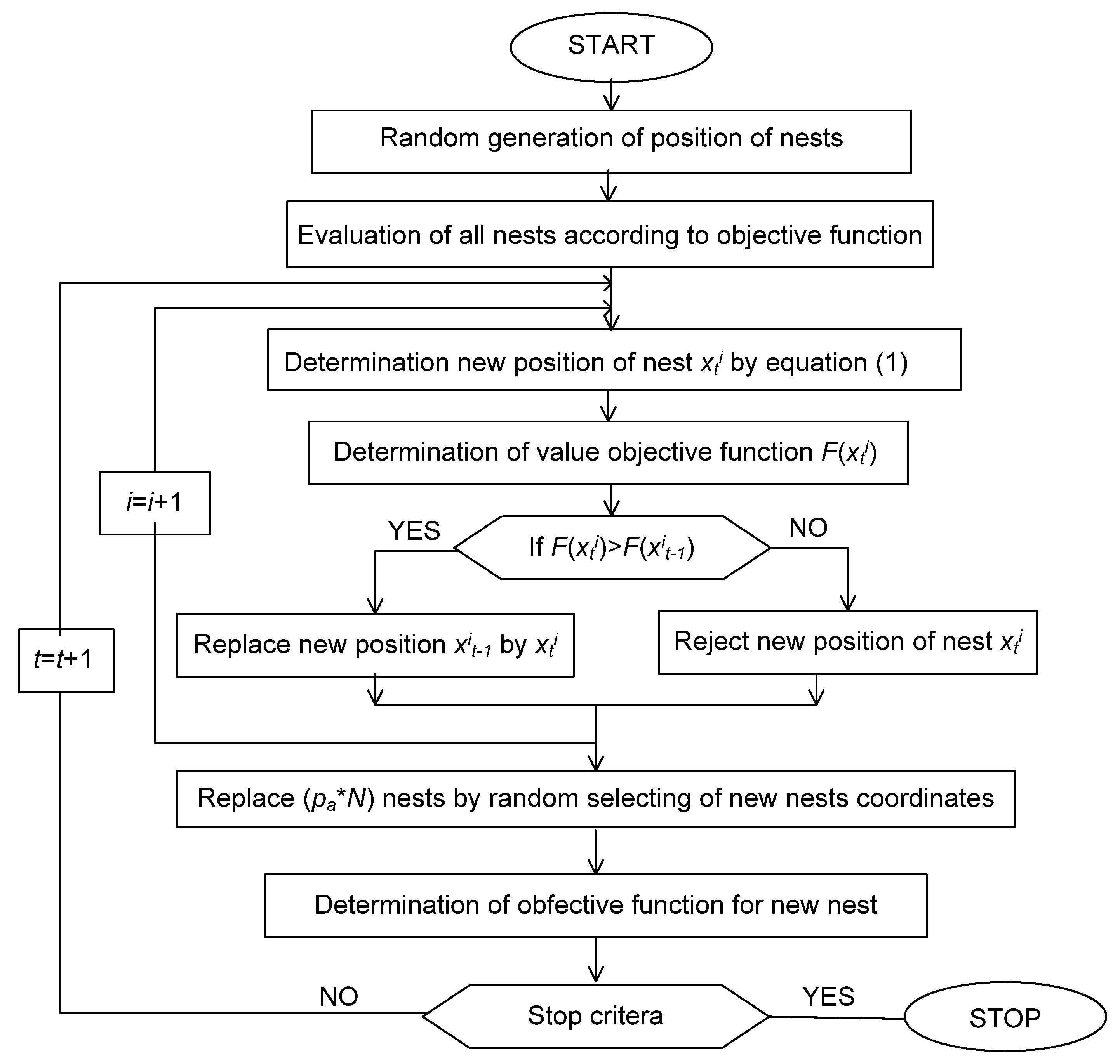
The block diagram (in the case of maximization) of the proposed algorithm is presented in
Figure 1. The maximum number of assigned iterations (
tmax) was adopted as the stop criterion.
2.3. Test of the Optimization Procedure Using a Test Function
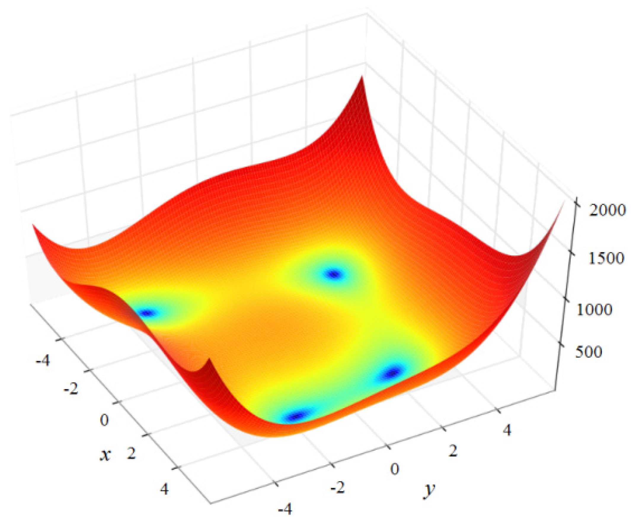
The optimization procedure was developed in Python 3.8. The correctness test was performed using the multimodal Himmelblau’s analytical function. The test function is defined by Equation (3):
wherein −5 ≤
x ≤ 5 and −5 ≤
y ≤ 5.
The Himmelblau’s function has one global maximum at the point (−0.270845, −0.923039), where
f(
x,
y) = 181.617, and four local minima at the following points: (3,2), (−2.805118, 3.131312), (−3.779310, −3.283186), and (3.58428, −1.848126). All local minima are identical and equal to zero (
f(
x,
y) = 0). The 3D visualization of Himmelblau’s function is presented in
Figure 2.
The optimization calculations were performed for the following parameters: there is a number of cuckoos equal to
N = 100, a number of nests equal to
n = 125, and a probability
pa = 0.25, while the maximum number of iterations is
tmax = 40. The optimization procedure was run 10 times, and the best results are presented in
Table 1. In each successive column is listed: the number of the iteration (
t), the
x and
y coordinates, the absolute error between the optimal and actual value of the objective function (Δ
f), and the number of calls to the objective function (
Nof).
On the basis of the results obtained from the CS algorithm, we can conclude that in the first iterations, the algorithm-determined solution approximates to the global extreme. The value of the objective function improves in successive iterations. After about eight iterations, a result is obtained which is close to the optimal one.
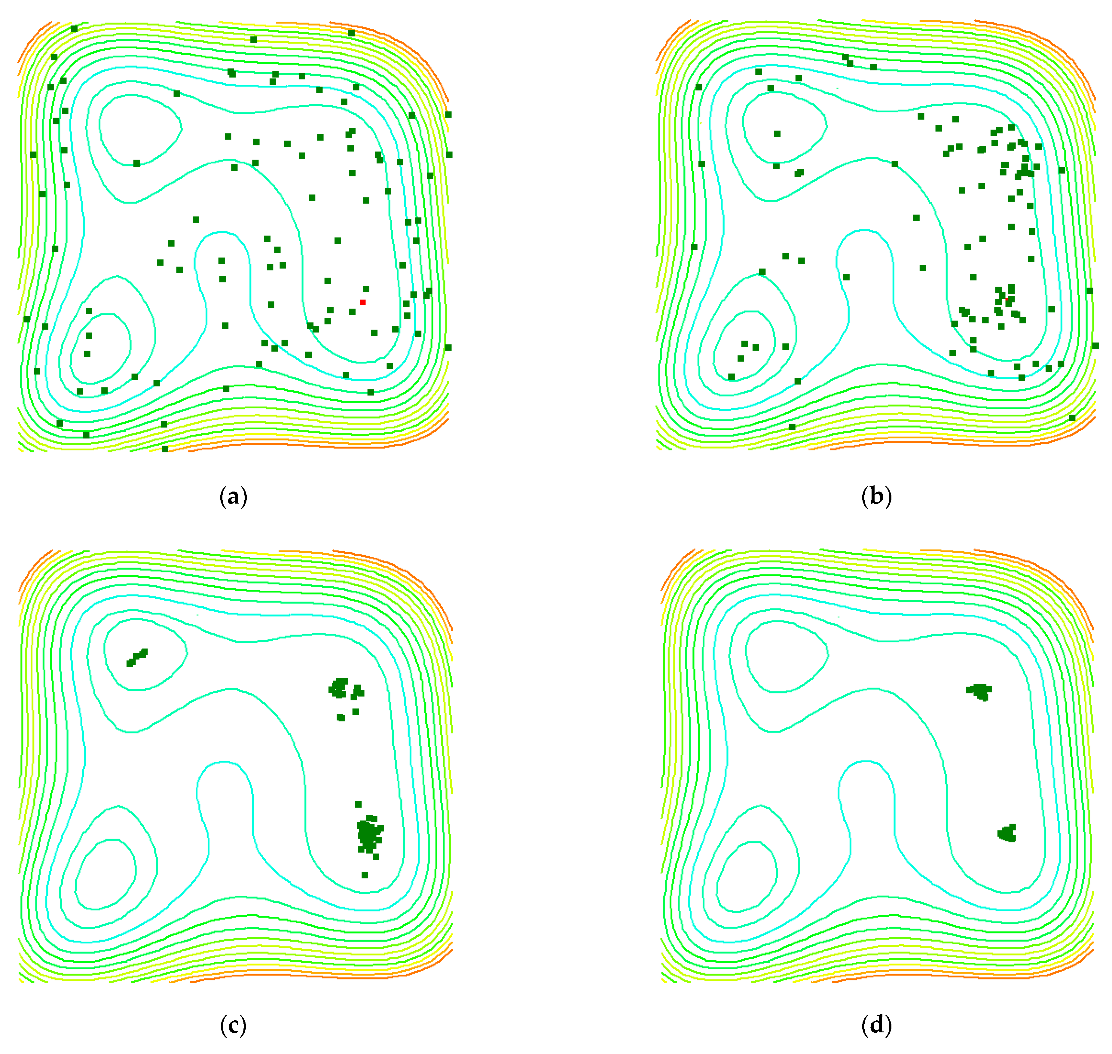
Figure 3 shows the distribution of the cuckoos in selected iterations of the algorithm. Based on the obtained results, it can be observed that after 25 iterations, the cuckoos are near three of the minimum points and about the same value as the objective function. After 40 iterations, all individuals are clustered near two minima points.
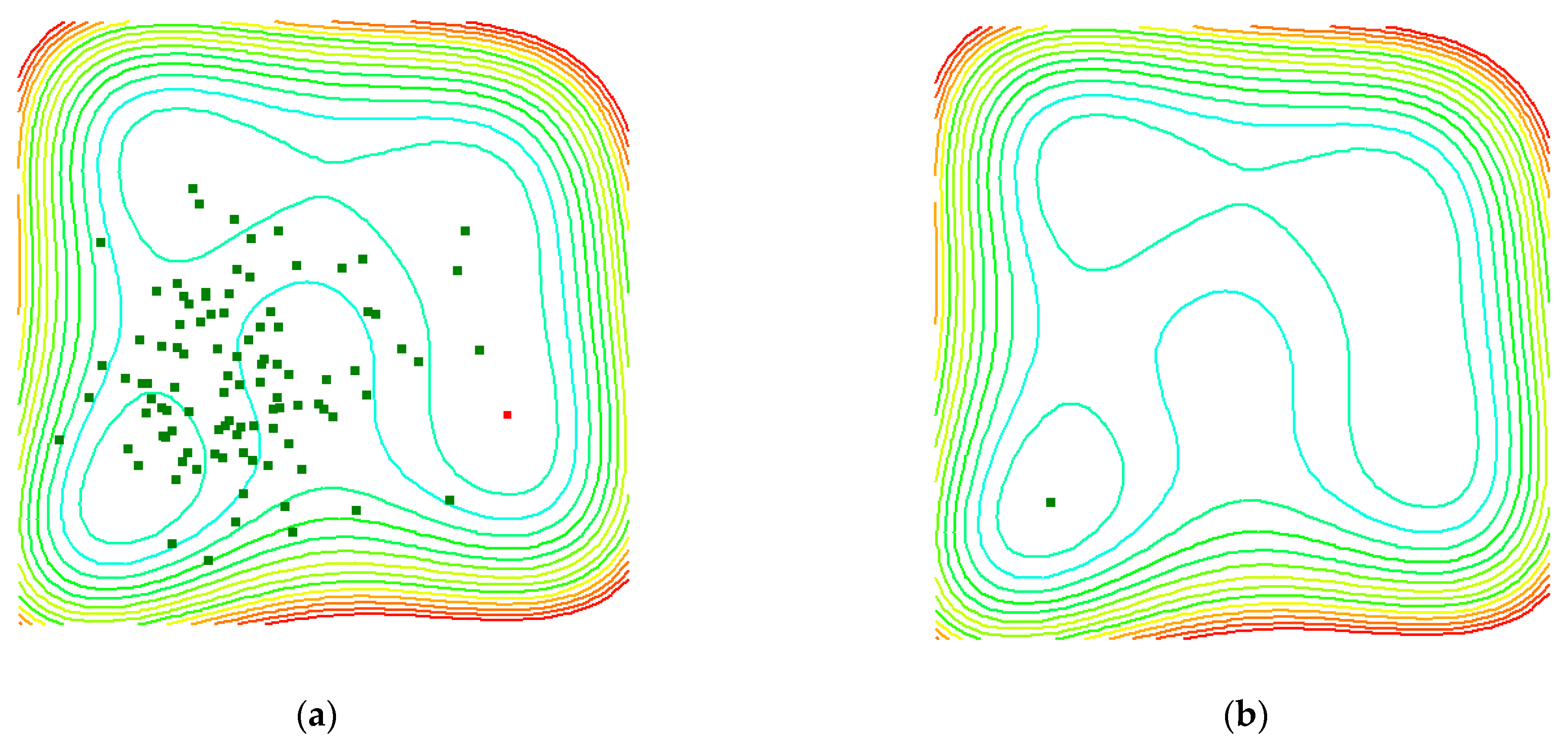
Figure 4 shows the distribution of the swarm particles in selected iterations.
Based on the distributions of the cuckoos (
Figure 3) and swarm particles (
Figure 4) in selected iterations, it can be observed that the process of searching for the global extreme is different. The PSO algorithm focuses on and goes towards the selected minimum, while the CS algorithm looks for a better extreme point throughout the whole optimization process.
If the optimization processes for the PSO and the CS algorithms are compared, it can be noted that for the PSO algorithm, all individuals in the swarm are moving towards a leader. On the other hand, for the CS algorithm, the process of focusing around the leader is much slower in relation to the PSO algorithm. Therefore, for the PSO algorithm, the external penalty function should be applied. The external penalty must systematically increase in subsequent iterations [
14]. In the case of the CS algorithm, a gentler way of considering constraints can be employed.
Here, the results obtained using the CS algorithm are compared with those obtained using the PSO algorithm [
31,
32,
33]. The calculations were repeated over ten runs for the same numbers of particles and a maximum number of iterations, as was the case for the CS algorithm. The following parameters of the PSO algorithm were applied:
w = 0.2,
c1 = 0.35, and
c2 = 0.45 [
14]. Additionally, the best, worst, and mean values of the objective functions and standard deviations for both algorithms were compared. The results are presented in
Table 2.
Table 2 shows that the best result for the CS algorithm is 0.002914, and for the PSO algorithm is 0.004196, which indicates that the best is lower for the CS compared to the PSO. Moreover, better standard deviation and mean values were obtained for the CS method. The CS method allows us to obtain a solution near to the optimal value for all runs, which demonstrates that the efficiency of the CS algorithm is good. Thus, the probability of finding the global extreme is greater for the CS algorithm.
3. Mathematical Model of the BLDC Motor
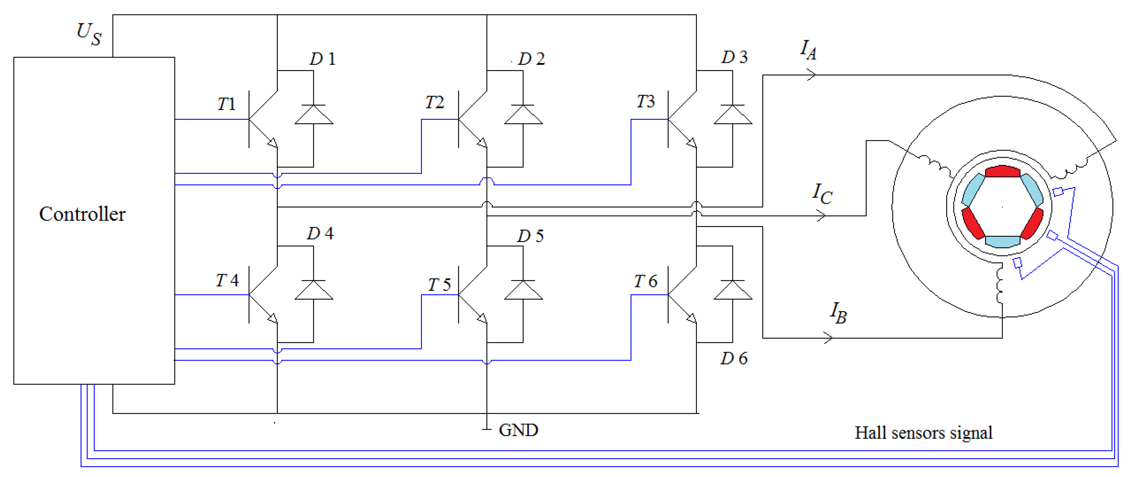
In the mathematical model of the BLDC model, it was assumed that there are three concentrated phase windings in the stator of the motor. The magnetic flux in the rotor is excited by the permanent magnets mounted on its surface. The structure of the motor and the system of the electronic commutator is presented in
Figure 5. The system of the electronic commutator is built from: (a) a microcontroller; (b) three Hall sensors; (c) six transistors (
T1–
T6); and (d) six diodes (
D1–
D6). The microprocessor supplies the transistor system with voltage
Us. The transistors distribute the voltage
Us on each BLDC phase winding.
The set of voltage equations for a three-phase motor are given in Equation (4):
where
uA,
uB, and
uC are the feeding phase voltage of the phases,
iA,
iB, and
iC are the phase currents,
RA,
RB, and
RC are the phase resistances,
,
and
are the flux linkages coupled with the phase winding
LAA,
LBB, and
LCC are the self-inductances of the phase windings,
LAB,
LAC,
LBA,
LBC,
LCA, and
LCB are the mutual inductances between phases, and
,
,
are the fluxes generated by the permanent magnets linked to the phase windings.
The distribution of the magnetic field excited by the permanent magnets depends on the position of a rotor [
33]. The flux linked with particularly concentrated windings made by the permanent magnets is recorded with the use of a dimensionless period function λ(α) defined in [
32], and depends on the number and volume of magnets used in a rotor, following Equation (6):
where
is the amplitude of the ‘linkage’ flux generated by the permanent magnets, and λ(α) is the dimensionless periodic function.
If the core of the BLDC motor stator is symmetrical, then Equation (7) is obtained according to reference [
34]:
where
M is the mutual inductance between the phases.
In the case where a winding is connected without the zero wire, the voltage equations are even simpler. The flux equation of phase
A is given by Equation (8):
and it is given in this matrix form by Equation (9):
where
is the vector phase inductance,
is the vector flux linkage,
is the vector of phase currents, and
is the vector of fluxes generated by the permanent magnets that are linked to specific windings.
The full set of voltage equations of the BLDC motor is, therefore, obtained by Equation (10):
where ω is the angular velocity of the rotor, and
is the vector of the phase supply voltage.
Assuming, that the electrical power generated in every winding is changed into mechanical power [
35,
36], the electromagnetic torque of the motor can be determined by Equation (11):
where
eA,
eB, and
eC are the values of back electromotive forces (EMF) inducted in particular phases [
31].
During the analysis of the dynamic states (starting or a load torque change), the rotational velocity was changed significantly. In this case, it is crucial to include the mechanical equilibrium equation in the mathematical model of the motor according to Equation (12):
where
J is the rotor’s moment of inertia,
B is the friction constant,
To is the load torque of the motor, and
T is the electromagnetic torque generated on the motor shaft.
One of the most important parameters of the permanent magnet motor in the steady-state analysis is the torque pulsation factor [
37,
38,
39]. In the proposed mathematical model, the pulsation factor is calculated by Equation (13) according to [
40]:
where
Tmax and
Tmin are the maximum and minimum torque values, and
Tav is the average torque.
4. Software to BLDC Analysis
The computer software for the analysis of the operating state of the BLDC motor was developed on the basis of the mathematical model described in
Section 3. The script has been developed in Python 3.8 and Windows 10.
Before starting calculations, the user has to provide the rated data of the simulated BLDC motor. All the simulation calculations were performed for the BLDC motor with catalogue number 57BLR50. The rated data of the motor are listed in
Table 3.
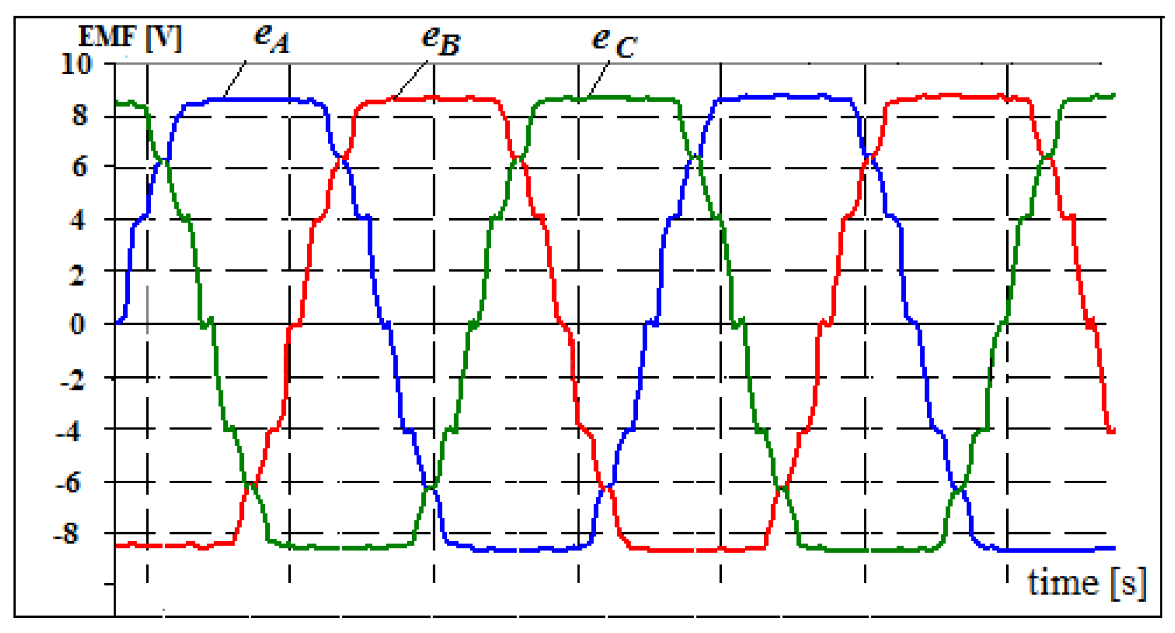
In order to avoid imperfections in the production process of real devices [
41], the values of the phase stator winding resistance, the self-phase inductance, and the mutual inductance between phases were determined by the use of the magnetostatic FEA model [
42]. The FEM mesh with 34960 triangular elements has been applied. The demagnetization curve of permanent magnets has been approximated by a linear function. The backelectromotive forces (EMF) for the stator winding were also determined to estimate the maximum value and obtain more accurate results in the simplified model of a BLDC motor. The waveforms of back EMF are presented in
Figure 6.
As a result of the FEM calculations, the following values were obtained: RA = RB = RC = 0.624 Ω, LAA = LBB = LCC = 1.123 mH and LAB = LAC = LBA = LBC = LCA = LCB = 4.26 μH.
Only some input data of the optimization procedure were determined by the use of the FEM model. The time of calculation of FEM parameters is less than 1% of the total calculation time of a single optimization procedure. Therefore, the numerical algorithm for determining the electromagnetic field that has been elaborated by the authors was applied. The algorithm was based on the Newton–Raphson process [
43]. There are more effective methods for calculating the electromagnetic field distribution [
44,
45]. Due to the relatively short calculation time, we did not use these methods.
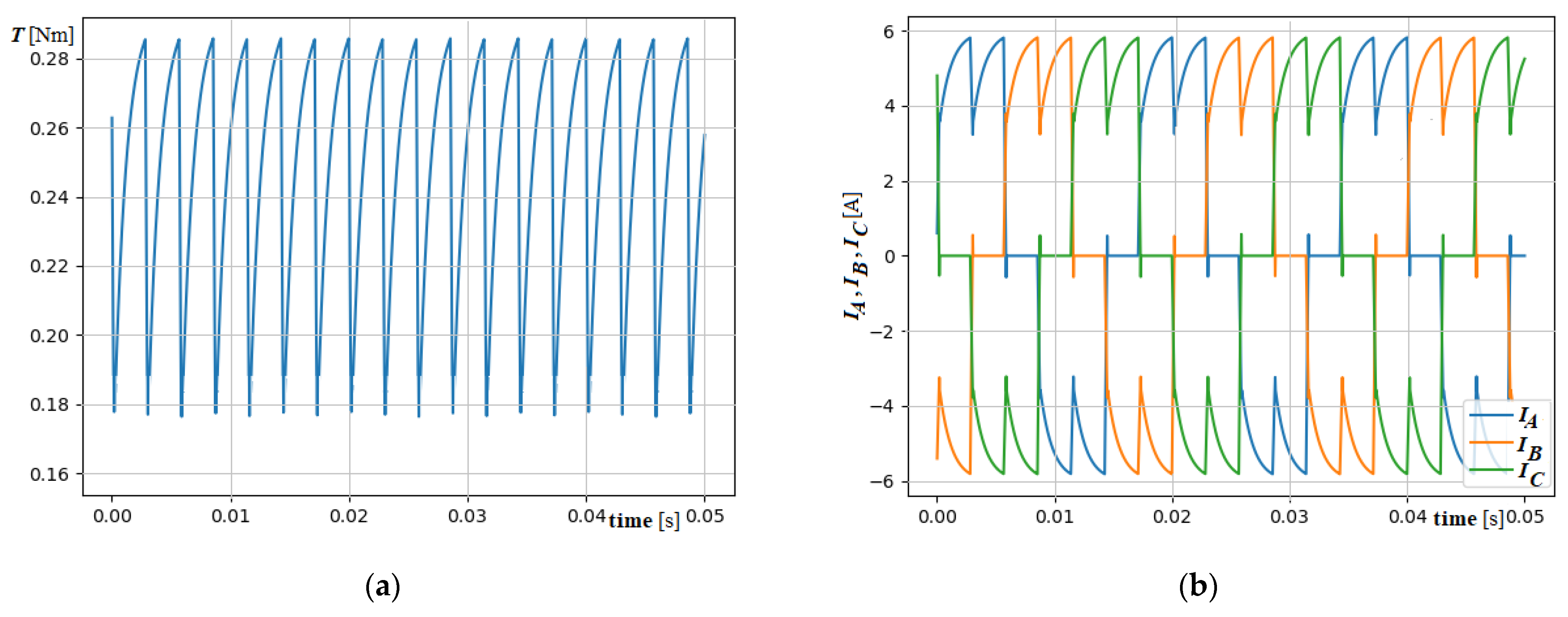
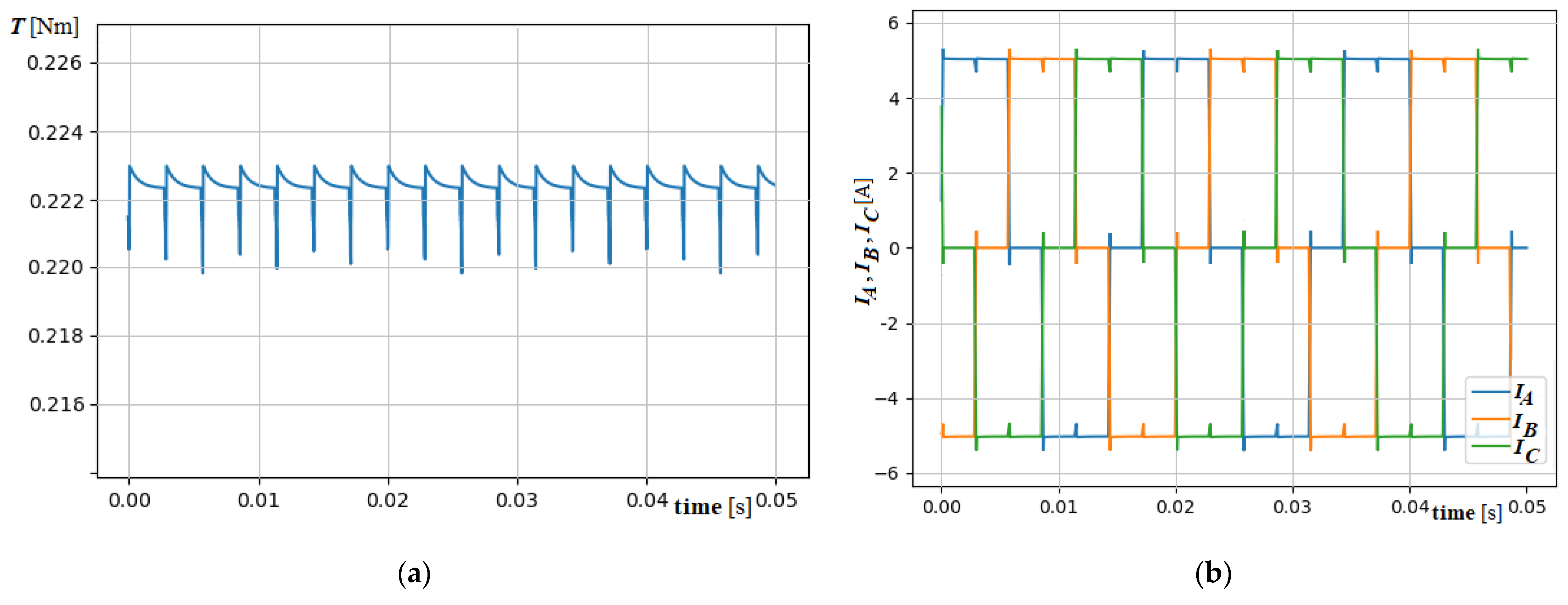
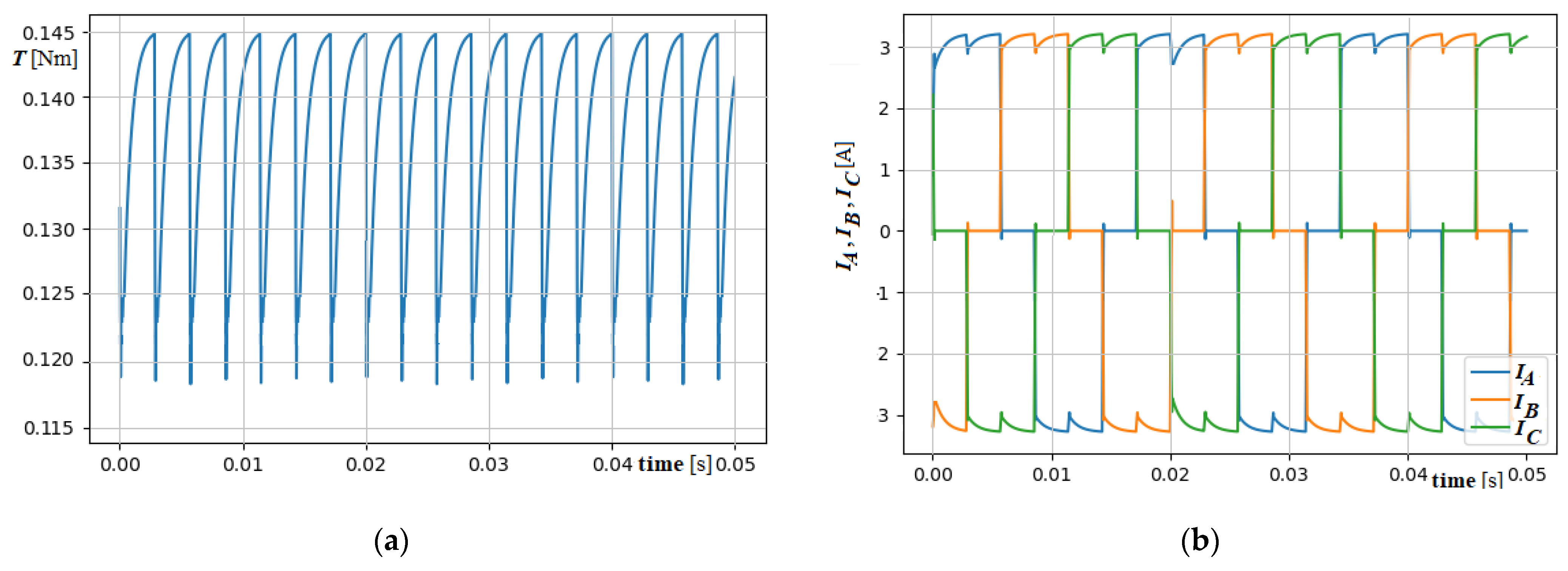
By using this software, the phase current waveforms and electromagnetic torque waveforms for the rated supply parameters and load torque equal to
TN were determined. The values of the rotor’s moment of inertia is
J = 128 g⋅cm
2, the friction constant is
B = 0.085 mN⋅m⋅s/rad [
46], and the time step length is Δ
t = 0.02 ms. These values were adopted. A waveform of the electromagnetic torque is shown in
Figure 7a. The waveforms of the phase currents for the rated torque are presented in
Figure 7b.
The value of the pulsation factor was determined for the simulation time to be ranging between 0 s and 0.032 s. The value of this factor is ɛ = 44.32%.
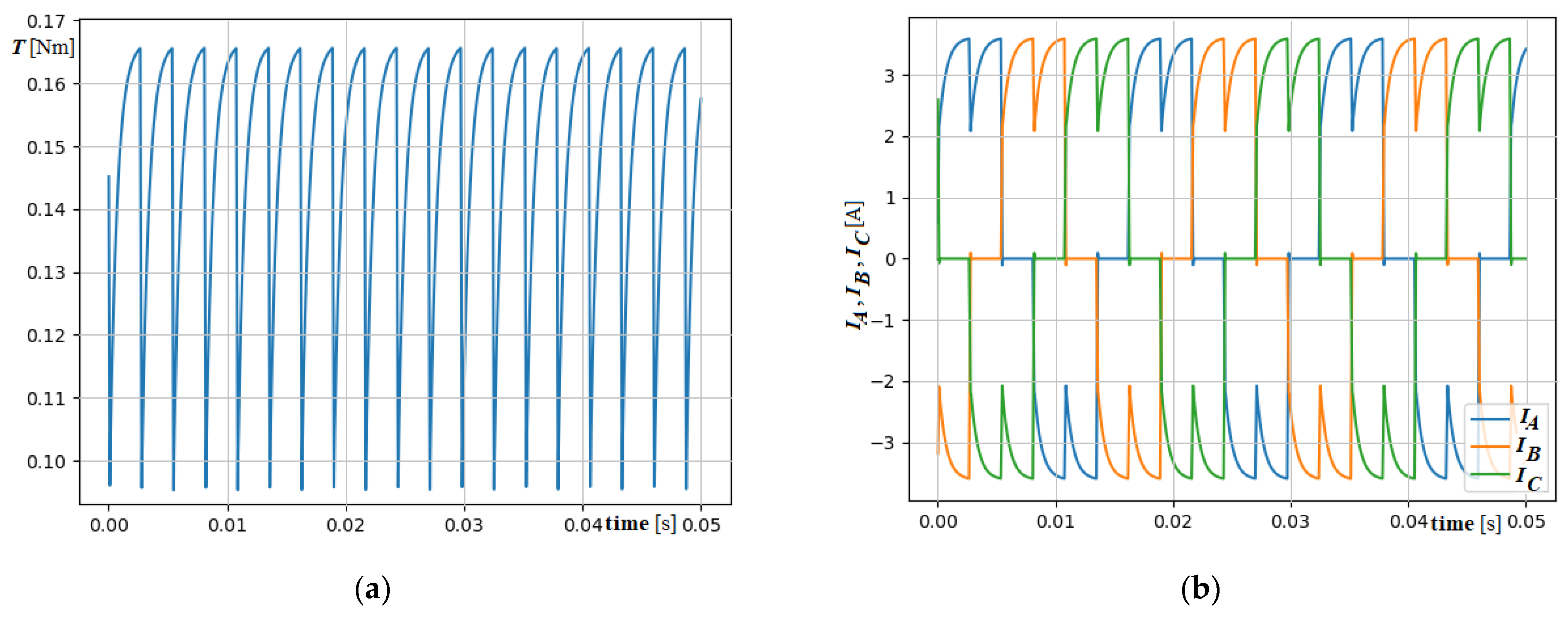
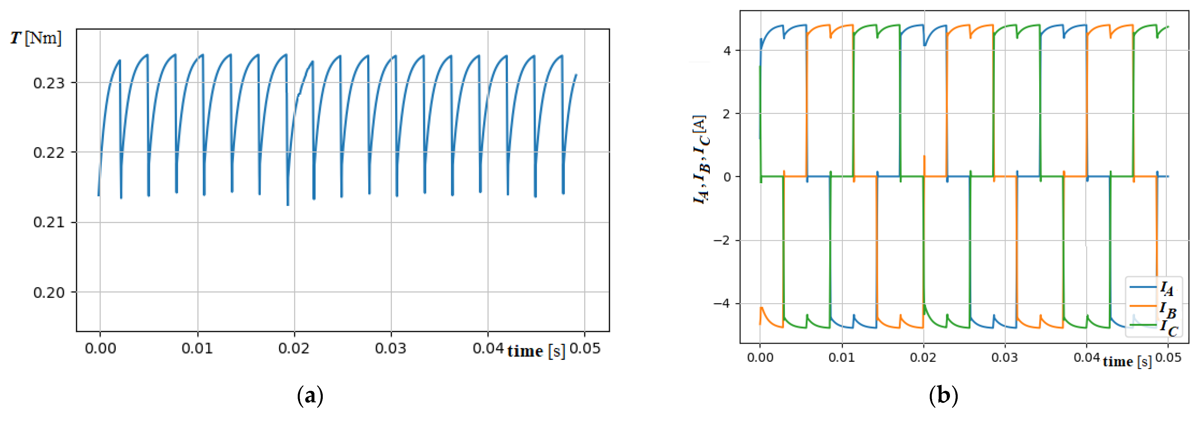
Then calculations were made with the value of the load torque at 0.6
TN, with ɛ = 53.19%. The resulting phase currents and electromagnetic torque are presented in
Figure 8.
The simulation calculations for different values of load torque and rotational velocity were performed. The obtained results of simulation calculations are presented in
Table 4.
Based on the simulation results presented here, it can be observed that a higher value of pulsation factors was obtained for the lower value of the load torque. A higher mechanical load increases the mechanical power on the shaft. At constant voltage, the test machine draws a higher value of current from the stator windings for a bigger load torque. The value of winding currents depends on the mechanical loading. In order to obtain a constant value of the pulsation coefficient in the BLDC motor, it is necessary to modify the value of the waveform’s supply voltages.
5. Formulation of an Optimization Problem
Torque ripples in the BLDC motors are caused by two different phenomena. The first source of torque ripple pulsation is related to interactions between the stator with slots and the permanent magnet rotor, referred to as the cogging torque [
47]. The second source of torque ripple pulsation is the commutation process during the exchange of current between the two phases [
48,
49]. The commutation torque ripple can even reach about 50% of the average torque generated by the BLDC motor [
49].
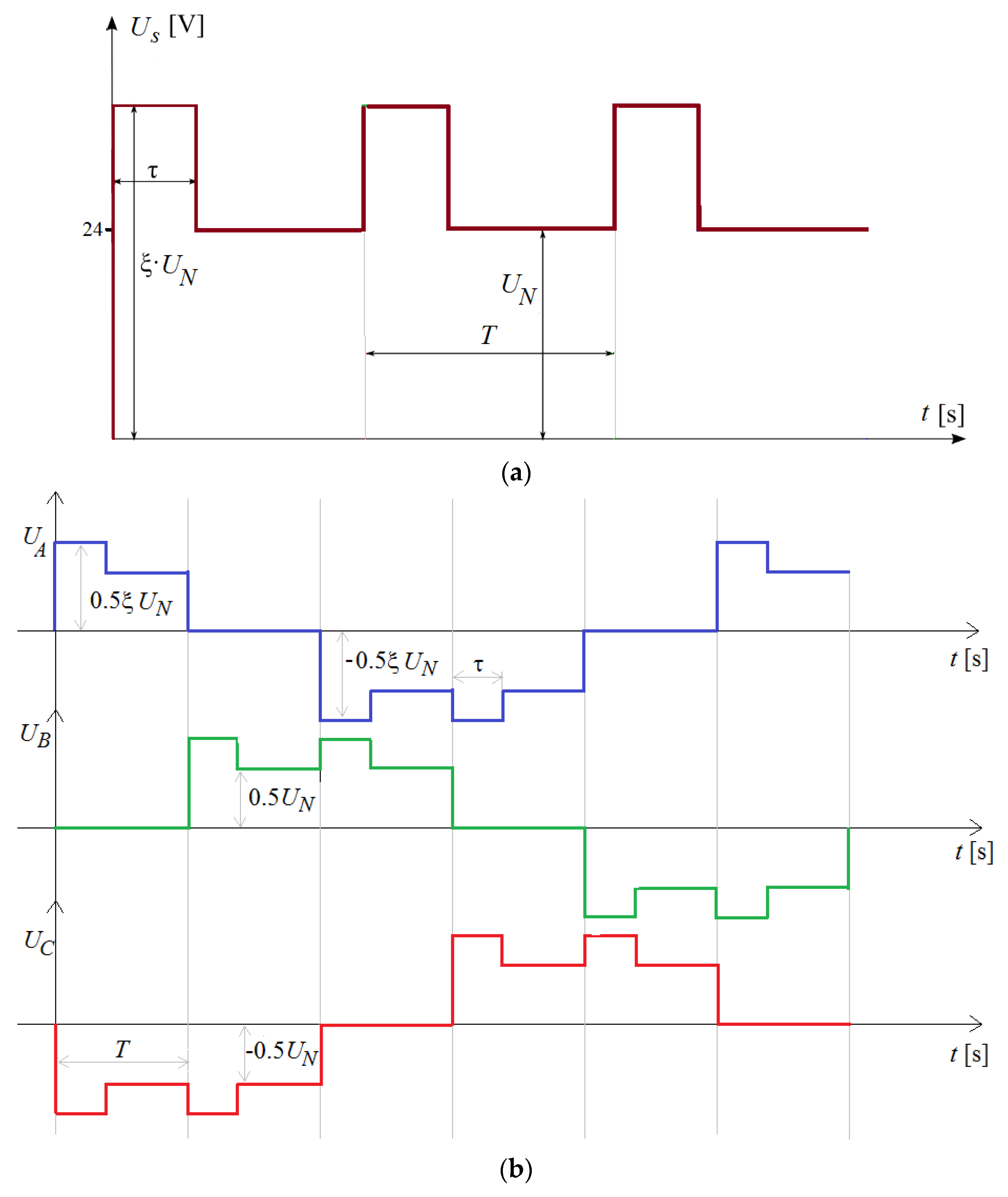
The optimization task consists of the selection of the two parameters describing the shape of a supply voltage waveform in order to obtain the maximum value of the average torque at the required value of the pulsation factor. Two design variables were taken into account:
s1 = ξ and
s2 = τ (see
Figure 9a,b). Design parameter ξ determines the value of the phase supply voltage in relation to the rated phase voltage, while variable τ defines the time in which the winding is supplied by increased voltage.
The supply voltage
Us waveform is generated by the microcontroller (see
Figure 5).
Us voltage is given to the electronic commutator. The controller controls the operation of an electronic commutator, i.e., a system of six transistors. The power supply to two phases of the stator winding is performed by switching transistors
T1–
T6 (see
Figure 5). The two phases of the stator winding are supplied by
Us voltage at any time. Then, the voltage on a single phase is equal to half the voltage
Us. The waveforms of the voltages (
UA,
UB, and
UC) on individual phases are shown in
Figure 9b. The phase voltages are input data in the mathematical model of the BLDC motor. They are used in Equation (4). The phase voltage values are calculated on the basis of the
Us waveform (see
Figure 9a). The shape of the
Us waveform is defined by two design variables,
s1 and
s2. The optimization procedure through the variables
s1 and
s2 influences the functional parameters of the motor, i.e.,
Tav and the pulsation factor ε.
The objective function for the
i-th cuckoo (the
i-th variant of the supply voltage waveform shape) is given by Equation (14):
where
Ti(
s1,
s2) is the value of the average electromagnetic torque for the
i-th cuckoo,
Tav0 is the value of the average electromagnetic torque after the generation of the initial positions of the cuckoos/nests.
The optimization problem consists of the maximization of the objective function (14) taking into account the permissible value of the pulsation factor
. In the case of the constrained optimization problem, the primary objective function
f(
s1,
s2) is modified by penalizing for overstepping the required constraints [
50,
51,
52]. Thus, the penalty term
p(
s1,
s2) is added to the primary objective function.
The constant static penalty approach has been taken into account in the developed algorithm [
53], and
p(
s1,
s2) is obtained by Equation (15):
where ε
i(
s1,
s2) is the value of the pulsation factor for
i-th the cuckoo, ε
p is the required value of the pulsation factor, and γ is the constant number dependent on solving the task [
54].
Finally, the modified objective function [
55,
56]
hi(
s1,
s2) consists of two components [
8] and is calculated for the
i-th cuckoo by the Equation (16):
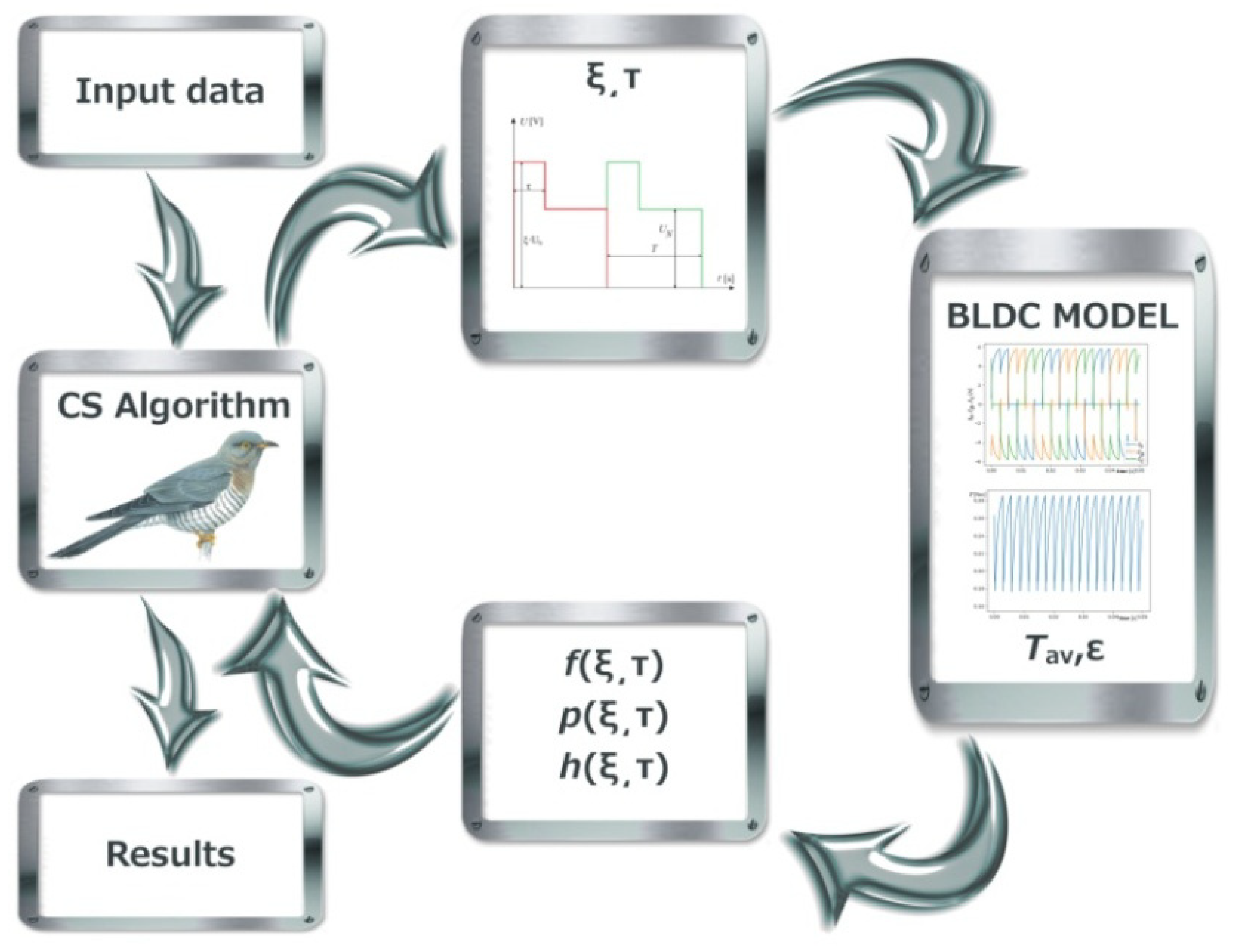
6. Results of Constrained Optimization
The constrained optimization calculations were performed using computer software developed in Python. The CS algorithm was selected to solve this optimization task. This is because in the last two years an increased interest in this optimization algorithm has been observed [
57,
58,
59]. The software was designed by the authors and consists of two independent and cooperating parts. The first part contains a mathematical model of the BLDC. The master module forms a optimization algorithm that manages the work of the mathematical model of the motor. A block diagram of the software is presented in
Figure 10.
Before starting on the optimization calculation, the user must declare the input data, which consists of: (a) the rated parameters of the studied BLDC motor; (b) self- and mutual inductance between phases; (c) the rotor’s moment of inertia; (d) the friction constant; and (e) the permissible value of the pulsation factors. Next, the optimization procedure is run. The procedure creates an initial population of cuckoos and executes the calculations for the declared maximum number of iterations. From each individual, the optimization procedure imitates the calculations of the mathematical model for the given design variables (s1 and s2). The module with a mathematical model calculated the values of the average electromagnetic torque and the pulsation factor. After the mathematical model finishes the calculation for i-th individual, the values of the primary objective function (fi), the penalty term (pi) and the secondary objective function (hi) are determined. The modified values of the above parameters (f, p, and h) are sent to the optimization procedure to evaluate of the i-th cuckoo.
In order to evaluate the performance of the computer software, a large number of simulations were conducted. The optimization calculations were performed for the following CS algorithm settings: the number of cuckoos is
N = 54 [
60,
61,
62], the number of nests is
n = 72, the maximum number of iterations is
tmax = 30, and the probability is
pa = 0.25. The value of the constant coefficient that determines the size of the penalty is γ = 0.55. For each of the analyzed permissible pulsation factors, five independent runs of the optimization software were carried out. The ranges of the design variables assumed during the optimization process are presented in
Table 5.
At the beginning, calculations were made for the required value of the pulsation factor ε
p = 5%. The optimization process was repeated five times for the different positions of nests. The best obtained result is presented in
Table 6. The course of the optimization process for the subsequent iterations of the CS algorithm is presented in
Table 6.
Based on the results obtained in
Table 6, it can be noted that the optimal solution was achieved after six iterations of the cuckoo search optimization algorithm. The subsequent iterations of the algorithm did not lead to any better-quality solution. It is necessary to point out that the best improvements concerning the pulsation factor were obtained between the first and second iteration of the optimization algorithm.
The waveform of the electromagnetic torque for the required ε
p is shown in
Figure 11a. The waveforms of the phase currents for the required ε
p are presented in
Figure 11b.
Next, optimization calculations were made for the less restrictive value of the pulsation factor, which is equal to ε
p = 22%. The optimization process was performed for the rated load torque at first. The optimization parameters for the selected iterations of the optimization algorithm are presented in
Table 7.
The waveforms for the optimal solution are presented in
Figure 12a,b.
Then, optimization calculations were made for the lower value of the load torque of 0.6
TN. The waveforms of electromagnetic torque and phase currents for permissible pulsation factor ε
p = 22% are shown in
Figure 13a,b, respectively.
Phase currents for the rated voltage (see
Figure 8b) and phase currents for the modified shape depend on the value of the load torque (see
Figure 13b). The average currents for loading torque equal to 0.6
TN are similar and do not depend on the pulsation factor. If we load machines by the same load torque, we will obtain a similar value of phase current. A similar phenomenon is observed for a brush DC motor, in which the current value is proportional to the load torque value.
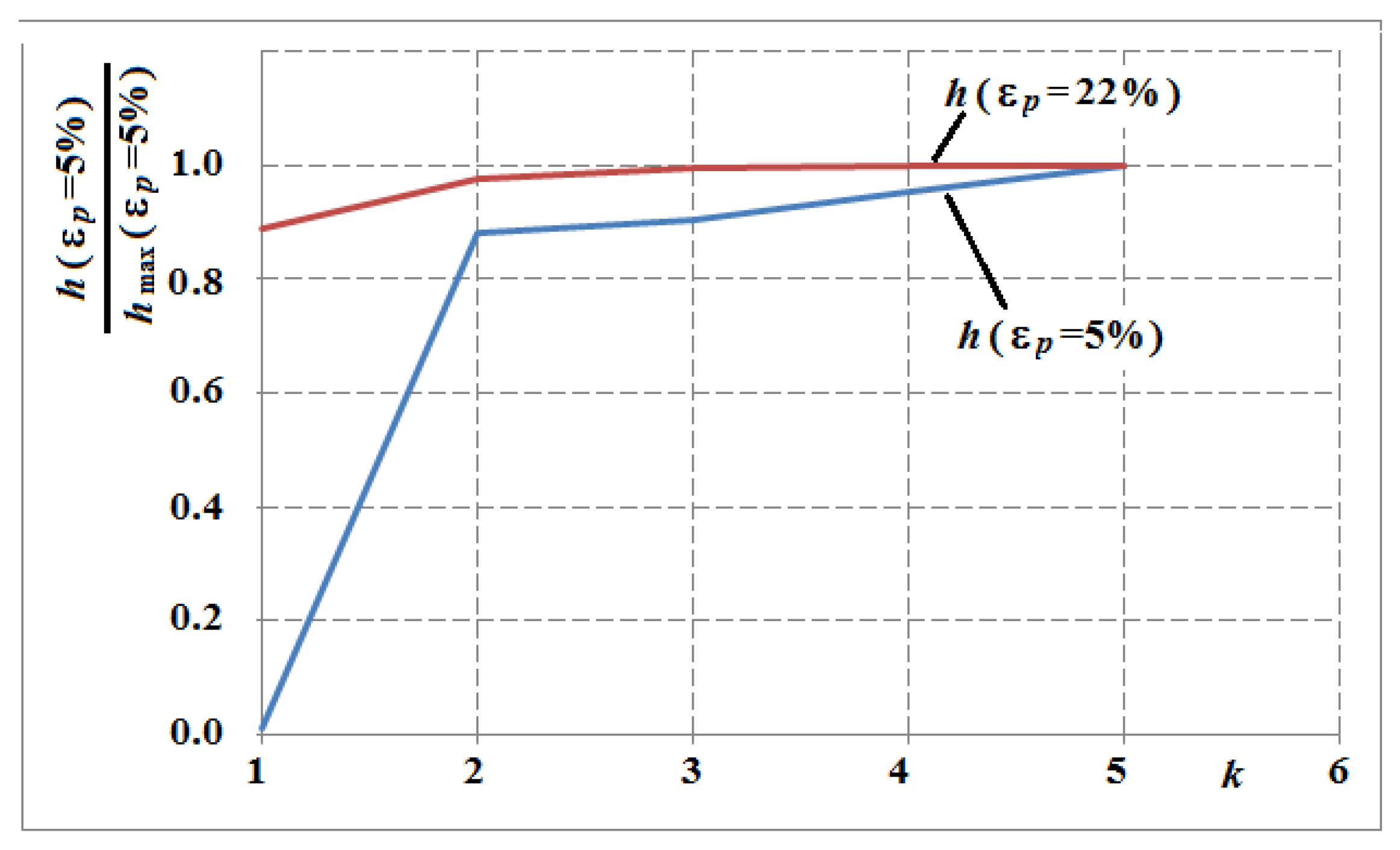
When comparing the courses of the optimization processes for the two different constraints, it can be concluded that, in the case of the less restrictive constraint (εp = 22%), the optimal solution was determined faster, i.e., after four iterations of the CS algorithm.
Figure 14 presents a comparison of the convergence curves for the two values of permissible pulsation factors equal to ε
p = 5% and ε
p = 22%. The figure shows the relative convergence of the modified objective function related to the optimal value. In the case of a gentler permissible pulsation factor, the result close to the optimal one will be obtained faster (see
Figure 14).
Finally, the optimal results of the constrained optimization for the different values of load torque were calculated. The permissible value of the pulsation factor was equal to ε
p = 22%. Five independent optimization processes for each load torque were made. The initial populations were selected randomly. The comparison of the obtained results is shown in
Table 8.
To achieve the permissible value of the pulsation factor of ε = 22% for different values of load torque, the various parameters (ξ and τ) describing the supply waveform should be applied. The analysis of obtained results shows that a high value of the pulsation factors requires the application of a higher modified supply voltage waveform.
7. Conclusions
The paper presents the application of the CS algorithm for the minimization of the commutation torque ripple in a brushless DC motor. The code was elaborated upon in Python for Windows. The structure of the computer software with all components has been presented in detail. The optimization task was the maximization of the average electromagnetic torque coupled with the constraint on the pulsation factor.
The obtained results of the computer simulation for the elaborated CS procedure are encouraging. Based on the presented results, in order to test the analytical function of a BLDC, the proposed CS procedure is much better in terms of effectiveness and quality when compared to the classical PSO approach. Moreover, according to the authors, the CS algorithm should guarantee a higher probability of finding the global extreme. After analyzing the optimization process for the CS algorithm, the static penalty function was applied to take into account the constraints.
The course of the optimization process was investigated for two different constraints: in the first case, a more restrictive permissible value of pulsation factor εp = 5% was imposed. The average value of the electromagnetic torque was 0.222, which is 5% lower in relation to the rated torque. The optimal solution was obtained after six iterations. In the second case, the optimization process was performed for the softer value of permissible pulsation factor εp = 22%. The optimal solution was obtained after four iterations of optimization algorithms, and the value of the average electromagnetic torque was 0.228. The obtained results confirm that for the less restrictive constraints the optimal solution can be found faster.
Based on the obtained results of the computer simulation, it can be concluded that the proposed approach allows obtaining the results of calculations with satisfactory accuracy with an acceptable calculation time. During the commutation phenomena, especially in supply systems with shaped values, there can be highly saturated subareas in the magnetic circuit of the motor. The difficulty is correctly estimating phase self-inductance and mutual inductance between two phases. Therefore, the values of the ξ coefficient must be carefully selected.
In future research, the authors want to focus on the design and execution of a laboratory stand to perform an experimental verification of research. Next, the performance of the CS algorithm will be compared with other heuristic optimization algorithms such as the genetic algorithm, particle swarm algorithm, or gray wolf algorithm. Moreover, additional constraint functions could be taken into consideration in future research to achieve a much more complicated constrained optimization task. Finally, the mathematical model of the BLDC motor will be expanded upon with thermal equations.


