1. Introduction
The shifting energy landscape and increasing demand for electricity are driving fundamental changes in the way power networks are being handled. Increasing renewable energy at the bulk system, along with decreasing inertia, are complicated challenges for Transmission System Operators (TSOs) [
1]. Several TSOs have reported the decreasing of inertia in their systems due to the large increase of renewables into the grid. For instance, in [
2,
3], the North American Electric Reliability Corporation (NERC) and Hydro-Québec TransÉnergie (HQT) both have reported a decrease in their respective system frequency response and inertia as a result of converter interfaced generation and recommended the use of synthetic inertia as a possible remedy. Similarly, academic studies have shown short-coming projections of the impact of inertia on the frequency and the synthetic applicability. A study of the Great Britain power network model in [
4] suggests the requirement of frequency ancillary services implemented in the network. Another system widely reported academically is the ERCOT, which has been dealing with several challenges lately [
5]. This system is working on analysing possible options to improve the frequency response including renewables and estimate future prospect to protect it.
One important indicator of the system frequency response following a system disturbance is the Rate of Change of Frequency (
RoCoF), which provides the gradient of changes in the frequency steps. Hence, this indicator plays an essential relationship in the stability and resilience of the grid [
6]. Moreover, the use of
RoCoF is not only crucial for the synthetic inertia control [
7], but for other applications such as the inertia estimation [
8,
9,
10], the
RoCoF sharing for enhancing primary controllers [
11], Wide-Area frequency measurements [
12], load shading schemes [
13], frequency stability margins [
14], and possibly, to determine the inertia placement [
15].
Several authors have investigated the possible challenges when measuring the
RoCoF since its behaviour might determine a possible loss of stability or poorly control performance. A study showing the impact of the
RoCoF location measurements is shown in [
16], the susceptibility of
RoCoF measurements to common power system disturbances such as phase steps is described in [
17], the settings of
RoCoF relays during islanding are studied in [
18], an on-line frequency estimator is proposed in [
19], and implementing a digital filter and consecutive data-points for inertia estimation and a comparison of frequency estimation techniques are explored in [
20]. A study of several variations of PLL for PMU application is presented in [
21], investigating the update rate of frequency and
RoCoF measurements with high accuracy under off-nominal frequency scenarios. In [
22], it is shown that the
RoCoF estimation error is primarily dependent on noise mechanisms in the input section and the adequate bandwidth of the signal processing algorithms. The authors of [
23] explore the impact of wideband noise on synchrophasor, frequency, and
RoCoF estimation. Using real-world acquisitions measurements, appropriate sampling, and the
RoCoF is studied in [
24]. In [
25], some consolidated window-based synchrophasor estimation algorithms schemes are tested on the frequency and
RoCoF measurements considering the threshold for load shedding. The application of the interpolated discrete Fourier transform (IDFT) and Kalman Filter (KF) in the estimation latency and estimation error of
RoCoF is evaluated in [
26], showing the rolling window period complexity in the calculation.
The calculation/implementation of the
RoCoF, as a discrete derivative of the frequency, has bandwidth limitations on the windowed response [
27]. Those limitations can definitely affect the performance of the
RoCoF performance in control systems, leading to excessive load restore actions or critically stable frequency regions. Thus, further studies of how the derivative calculation of the frequency impacts the
RoCoF accuracy and tolerance are necessary.
As the rotational inertia of the power system is reduced, the importance of providing mechanisms to manage the frequency response becomes extremely needed to keep the operational security level of the synchronous dominated power systems. Inertia emulation control loop in power electronic converters is one of the mechanisms widely claimed as the solution of the low rotational inertial power systems. This paper investigates the inertia response and rate of change of frequency in a low rotational inertial scenario of a synchronous dominated system. This paper differs from many scientific papers on the topic of low rotational inertia as it is not intended to analyse the response of frequency sensitive control loops of power electronic converters. This paper considers the power systems to be dominated by the presence of synchronous generators, but the rotational inertia is reduced, and from there, the system frequency response is analysed. This paper differs from many other papers published on the topic. This paper is interested in explaining the physic and basic principles behind the low rotational inertia scenarios’ system frequency response, and particular emphasis is made on qualitative explanations using illustrative numerical experiments. The scientific paper is divided into seven small sections.
Section 2 is dedicated to presenting a general overview of the frequency in traditional power systems; it includes a discussion about the multi-layer control loop used in synchronous dominated power systems, then the section presents the main indicators used to assess the frequency response of the power system.
Section 3 presents a comprehensive discussion about the effects of reduced rotational inertia in the frequency response of traditional power systems with a special focus on two main aspects, the frequency response and the
RoCoF evolution after an under frequency event.
Section 4 defines the role of the rotational inertia of the synchronous generator in the system frequency response. One important aspect of this section is a discussion about how the size of the rotational inertial of individual generators may be different depending on the power system. A brief description of the rotational inertia of individual generators in two different countries in South America is presented (Chile and Peru). Then,
Section 5 presents a very comprehensive and qualitative explanation of the inertial response of individual generators. A simple experiment is used to compare the inertial power and energy provided by five different synchronous machines. This section concludes by explaining one of the potentially negative aspects of the inertial response of uncontrolled (no governor) synchronous generators, that is, the potentially risky situation where the synchronous generator recharges the kinetic energy of the rotor by taking power from the power systems during the course of the under-frequency event. The authors consider this explanation one of the most important contributions of this paper, as many implementations of the inertial response on power converter-based technologies do not consider the potentially harmful situation of draining active power from the power system during an under frequency event, a situation where totally opposite behaviour is need, e.g., power injection is desirable to establish the balance generation/demand. Finally, the authors dedicated a complete session to discuss two important aspects of the rate-of-change of frequency (
RoCoF): (1) An illustrative demonstration effect of the method and size of the moving window on the
RoCoF and (2) An illustrative example of using real measurement of system frequency obtained from phasor measurement using to demonstrate the noise implications when calculating the
RoCoF. This paper closes with a section dedicated to the conclusion and closing remarks. The authors recognise that the presentation of this paper is very atypical, but they want to present in a straightforward and illustrative way several relevant aspects of the inertia response and
RoCoF calculation that could help to understand and explain implementation and results of inertial response control implementation on power converter based technologies.
2. Frequency Traditional Power System
This section is dedicated to providing a comprehensive and practical understanding of the frequency control and system frequency response in traditional (synchronous machine-dominated) power systems and the main indicators used to analyse the performance of the system frequency response.
Electrical frequency is a vital variable in defining the operation of any alternate current (AC) electric system [
7]. In electrical power systems, the so-called nominal or rated frequency (
f0) specifies the characteristic of an apparatus upon which test conditions and frequency limits are based, and the system frequency (
f) is the frequency which a power system normally operates [
28].
The rated frequency of an electrical power system varies by country and sometimes within a country; most electric power is generated at either 50 Hz or 60 Hz. The frequency deviations from the rated frequency in a traditional power system are typically caused by active power imbalances between generation and demand. As a consequence, the classical assumption of system frequency constant is not real; in fact, the frequency is a highly variable electromechanical variable that follows the active power imbalances in the power system. The electrical system frequency is a continuously changing electromechanical variable. Therefore, it must be estimated and controlled in real-time in order to ensure a satisfactory balance between system demand and total active power generation.
When an active power change happens at one point inside of a multi-machine power system, this active power change propagates throughout the entire power system, forcing a necessary change of the electric frequency. Hence, the electrical system frequency is used as a valuable index to define the appropriate balance of the system active generation and load demand.
The electrical frequency deviations from the rated or nominal frequency are caused by an instantaneous imbalance between the instantaneous active power production and the load demand; the immediate effect is the acceleration or deceleration of the synchronous machines directly connected to the electrical power system and as a consequence modifying the system frequency. Considering normal operating conditions of the power system, small deviations of electric frequency are caused by the stochastic variations in the power demand of the load, and they must not impact the dynamic behaviour and performance of any component in the power system. The appropriate design, operation, and control of the electrical power system must ensure that system is able to handle those changes at any time scale.
The electrical power system is equipped with a specialised set of control loops dedicated to frequency control. Those control loops are accountable for maintaining the real-time balance between the changes in load and generation; the control function of the frequency control is to ensure a frequency inside the quality standards (as closest possible to the rated or nominal frequency) at any period of time. The frequency control is a crucial element in preserving the system frequency stability, which is defined as “the ability of a power system to maintain steady frequency following a severe system upset resulting in a significant imbalance between generation and load”.
Frequency stability analysis focused on analysing the overall system stability for sudden changes in the generation-load balance (system frequency disturbance, SFD). Additionally, the frequency control has particular importance under abnormal operating conditions; it is in charge of limiting the frequency deviations that arise following a large SFD, e.g., the loss or disconnection of a large generator, the abrupt interruption of heavily loaded transmission line, along with then ensuring the system frequency returns to the nominal or rated value within the expected time. The abnormal frequency conditions are accomplished using occasional frequency control services.
The frequency response (FR) is an automatic change in active power output or demand consumption as a response to a frequency change. The FR might be naturally provided or intentionally provided. Frequency sensible load must naturally change the active power consumption when frequency changes, this change are typically represented by an active power-frequency dependence and time constant. On the other hand, FR can be intentionally provided by a set of measures, but the main idea is to maintain system frequency within statutory and operational limits. Intentional FR is typically considered an auxiliary service in most of the power utilities and is financially compensated. In general terms, the system RF (SFR) refers to the measure of the power system to stabilise frequency immediately following an SFD.
Frequency control can be considered to be one of the most crucial aspects of ancillary services; it is responsible that the power system operates within its acceptable frequency limits [
29]. Frequency control practices differ significantly between the various transmissions system operators in the world [
30]. The classical approach to frequency control can schematically be divided into three: primary, secondary, and tertiary control (some specific applications are also called quaternary frequency control systems). The tertiary control is typically supplementary with very slow response than the other two controllers: primary and secondary frequency control. A specific and detailed explanation of the frequency controls in the traditional power system can be found in very well-known books as [
31,
32].
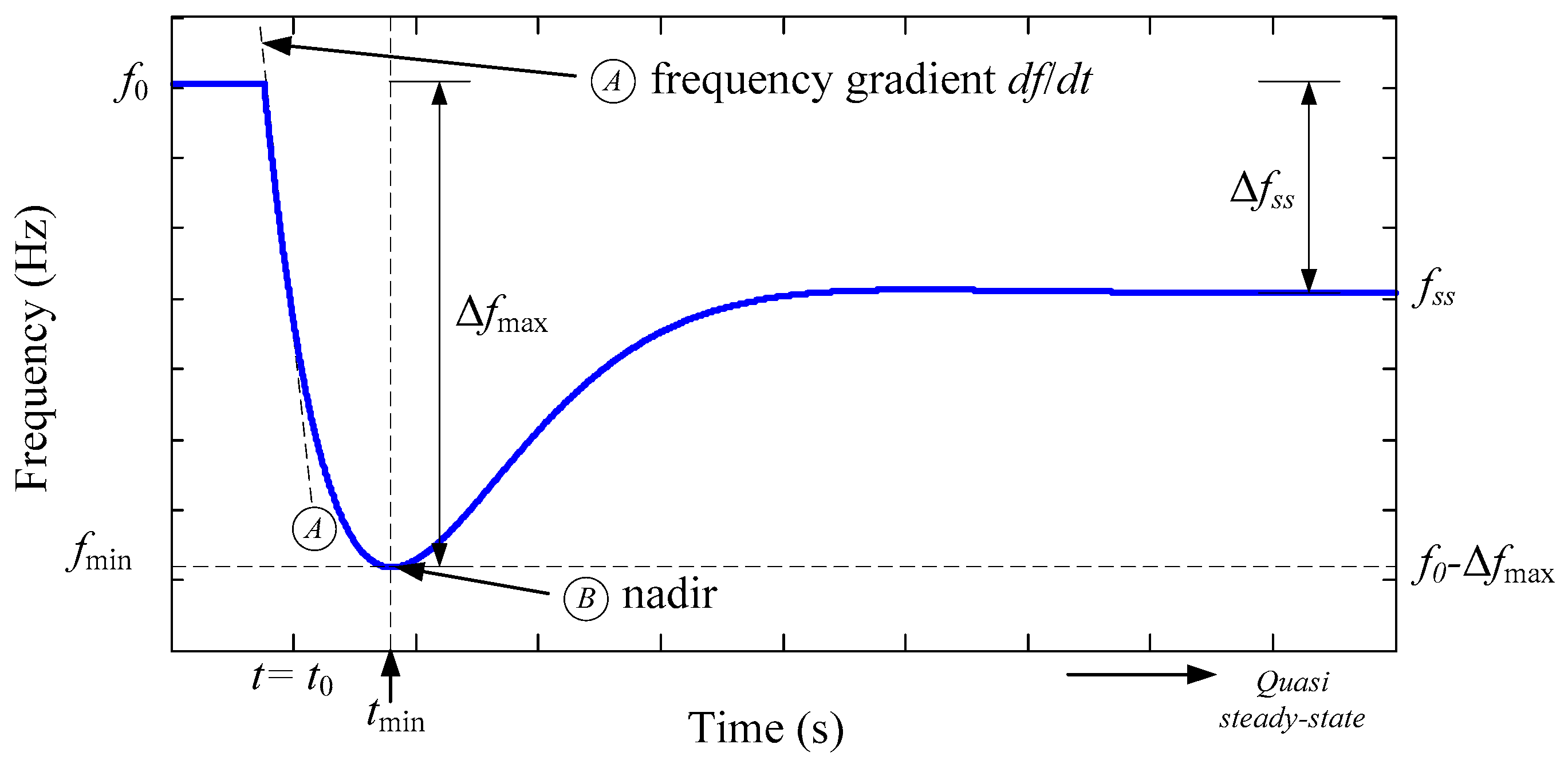
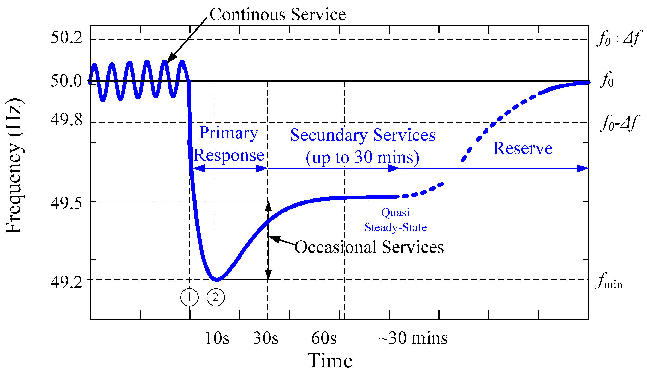
Figure 1 shows an illustrative example of the system frequency behaviour following an SFD (i.e., in this very specific case, an under-frequency event, sudden loss of generation or connection of a large load, at
t = 0 s). The numerical values of the rated frequency (
f0), acceptable frequency deviation (Δ
f), and minimum frequency shown in
Figure 1 are based on the illustrative case of frequency control in GB.
Several performance indicators may be used to describe and evaluate the FR.
Figure 2 shows a typical and idealistic SFR (secondary and tertiary control are not included) where the main performance indicators are depicted:
df/dtmax: Maximum frequency gradient defines the velocity of the frequency change over time, it is as observed by RoCoF relays (line ❶).
fmin: Frequency nadir or minimum frequency measures the minimum values of the frequency during a post contingency frequency (point ❷).
Δfmax: Maximum frequency deviation (Δfmax = f0 − fmin) is defined as the as detected by the traditional under-frequency (RF) protection relays (point ❷), it represents the absolute frequency deviation from nominal frequency (f0), Δfmax = f0 − fmin.
Both these system frequency response indicators must be controlled and reduced as much as possible in order to prevent the relays df/dt protection relays from tripping.
tmin: The time required by the system frequency response to reach its frequency nadir (fmin); it is also called frequency nadir time.
Δfss: Quasi-steady-state deviation defines deviation between the nominal or rated frequency value (f0) and the quasi-steady state frequency (fss).
Instantly following an SFD, the system electrical frequency drops (it is shown in the region ①–② of
Figure 2) at a rate primarily defined by the total system rotational inertia (summation of the inertia constant of all synchronous generators directly connected to the grid and spinning loads). During the operation of the power system in normal conditions, the system electrical frequency drops further outside of acceptable frequency deviation (Δ
f = ±0.20 Hz, GB case), and some generating plants are contracted to deliver frequency response. This kind of frequency response is categorised as an occasional service, and the frequency response has two components: primary response and secondary response. Those components are characterised by the additional active power that can be delivered from a generating unit to fulfil the frequency response service, In the very specific case of the GB system, the operational code requires that the additional active power must be available at 10 s and 30 s respectively (primary and secondary response) measured form the insertion of the frequency event and the code also requires that the provision of active power must be sustained for an additional 20 s and 30 min respectively [
30].
The primary frequency response is recognised to have two fundamental mechanisms: (i) Inertia response and (ii) Governor action. The primary frequency control is specifically dedicated to controlling actions that are performed locally (inside the local power plant) based on the set-points for electrical frequency and active power generation. The control objective of the primary control is very simple: the control actions are dedicated to maintaining the generation/load balance. This active power balance is reached by a balance between the electrical demand at the generation unit and the primary mechanical power applied to the generation unit, if frequency-stable, the steady-state post-disturbance frequency is reached, and it is different to the nominal or rated frequency. It is important to mention that this control includes a proportional control action that has a determinant effect in the steady-state frequency; it is the so-called droop characteristic (it may be present or not at the governor). The frequency control responsibility is shared between all the synchronous generators participating in the primary frequency control, irrespective of the location of the disturbance.
The inertia response is a natural phenomenon of the synchronous machines directly connected to the power system, and it is related to the energy balance of the electromechanical energy conversion system. For instance, during an under frequency event, the frequency reduction will cause a reduction in the rotational speed of the synchronous generator and the inherent physical rotational inertia characterising the rotor will try to keep the rotational speed of the rotor; as a consequence, some of the kinetic energy (KE) stored in the rotating mass (rotor) is released in the form of electrical energy. The inertia response is a very fast but natural behaviour found in the synchronous generator (SG) directly connected to the grid during an (under or over) frequency event. The inertia response of an SG depends on the rate of change of frequency (RoCoF). The SG provides the inertia response in natural and instantaneous. There are no measurement devices or controllers involved in this response, but it is extremely important for frequency stability.
A classical SG based generation unit is equipped with a frequency controller named governor; it is responsible for the so-called governor action (region ②–③ of
Figure 2). The governor controller is a local controller installed at the SG, and it is based on the electromechanical properties of the prime-mover (e.g., hydropower, thermal unit, etc.). An automatic droop control loop in the governor acts on frequency change and increases mechanical power on prime-mover to increase the generator output. The governor control action is a local is a slower response and depends on main governor’s characteristic and time response of prime-mover.
Following the under-frequency event caused by a SFD, the inertial response and governor action take place; if the power system is frequency-stable, the system frequency will not be able to return to the nominal frequency on its own without additional action.
The secondary frequency control (shown as the region ③–④ of
Figure 1), also called Load Frequency Control (LFC), modifies the active power set-points of the synchronous generators in order to counteract the electrical frequency error (frequency destination from the rated or nominal frequency) following the primary frequency control action [
33]. The control objective of the secondary frequency control actions restoring the electrical system frequency to the nominal set point and may involve the responsibility of ensuring that the power flows at a pre-defined tie-line in the system is inside the operating limits [
32]. The LFC actions might be implemented manually by humans, that is, the current status of the LFC in the Nordic power system. However, automatic implementation of the LFC is favoured by several countries around the world; for instance, the ENTSO-E Continental Europe interconnected system uses an automatic LFC scheme it is called Automatic Generation Control (AGC). LFC is the generic name of the controller but when automatic implemented that is called AGC.
The tertiary frequency control is very specific frequency control, and it acts after the system frequency have been returned nominal value, or it is around this value. The control objective of the tertiary frequency control is highly specific, and it is highly dependent on the organisational structure of the power system, and the given role of the power plants play in the power system [
31]. The tertiary frequency control differs from primary and secondary frequency control because it does not deal directly with controlling the frequency. The tertiary frequency control is not considered in this scientific paper and, because of that, is not discussed here.
After a severe SFD (e.g., significant generation loss), the power system frequency drops instantaneously as the remaining generation power no longer matches the active power load demand. A severe SFD, like a significant loss of generating the plant, without appropriate system frequency response can produce extreme frequency deviation potentially dangerous for the operation of the power system. If the frequency deviation reaches a prohibitive pre-defined threshold, emergency control and protection schemes may be required to regain control of the system frequency.
A typically used emergency frequency control is the under-frequency load shedding (UFLS). The UFLS is extensively used in electrical power systems as the last resource to protect the integrity of the system against significant low-frequency events that may cause cascading outages and finally result in a partial or total blackout. The objective control of UFLS strategy is to reestablish the generation/demand balance by appropriately disconnecting excess load during an under frequency event to ensure the supply can rapidly match the remaining demand and avoid cascading events that can degenerate into a partial or complete blackout.
3. Effects of Reduced Rotational Inertia in Traditional Power Systems
This section is dedicated to providing a quick overview of the effects of reduced rotational inertia in traditional, synchronous generator dominated power systems. This section uses an illustrative example to show the effect on the system frequency response and the RoCoF.
The growing interest in reducing CO2 emissions and reaching a zero-net emissions society motivates the massive integration of more environmentally friendly generation resources, e.g., wind power plants, solar PV power plants, etc. The majority of those weather-dependent generation units utilise power electronic converters (PECs) in the grid. Now, there is increased penetration of renewable-based generation using equipment with PECs and the disconnection of large synchronous generator-based generation units (scheduled and unscheduled decommissioning of polluting or aged power plants). As the number of synchronous generators directly connected to the power system reduces, the total rotational inertia of the power system is reduced. However, the electrical power system is losing more than rotational inertia. The rotational inertia is a natural and inherent electromechanical property of the synchronous generator. However, the power system looks at the number of synchronous generators and all the positive effects from the synchronous machine (e.g., short circuit contribution, overload capacity, etc.).
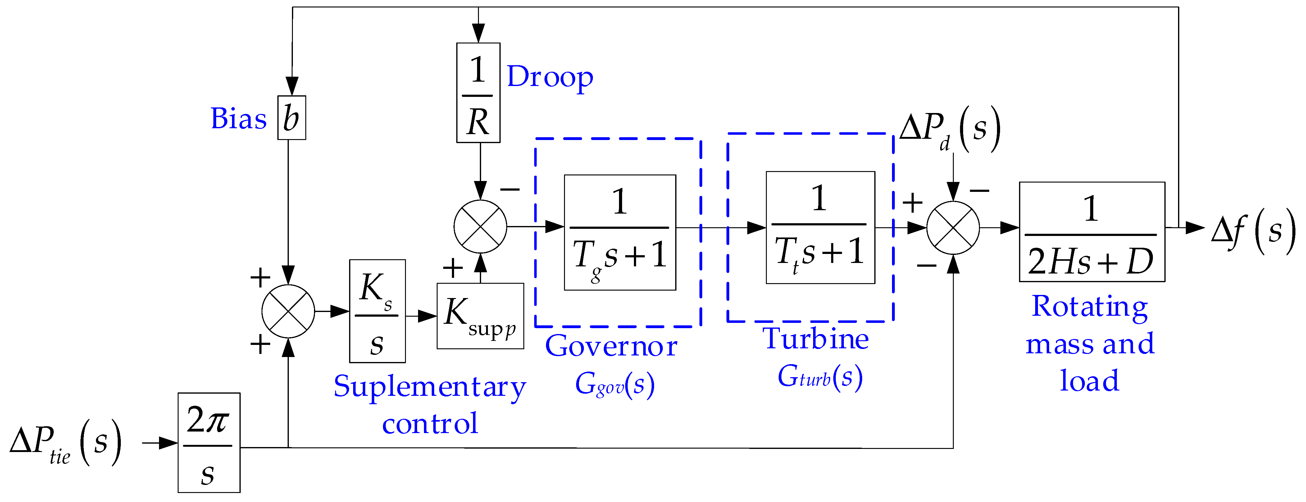
To illustrate the effects of reduced rotational inertia on the system frequency response of the electrical power system. A single area power system is analysed; it consists of an equivalent generator represented by rotational inertia (
H) and power demand of the frequency-dependent loads (
D). In reference to
Figure 3, the
Ggov(
s) is the transfer function of the governor,
Gturb(s) is the transfer function of the hydro turbine.
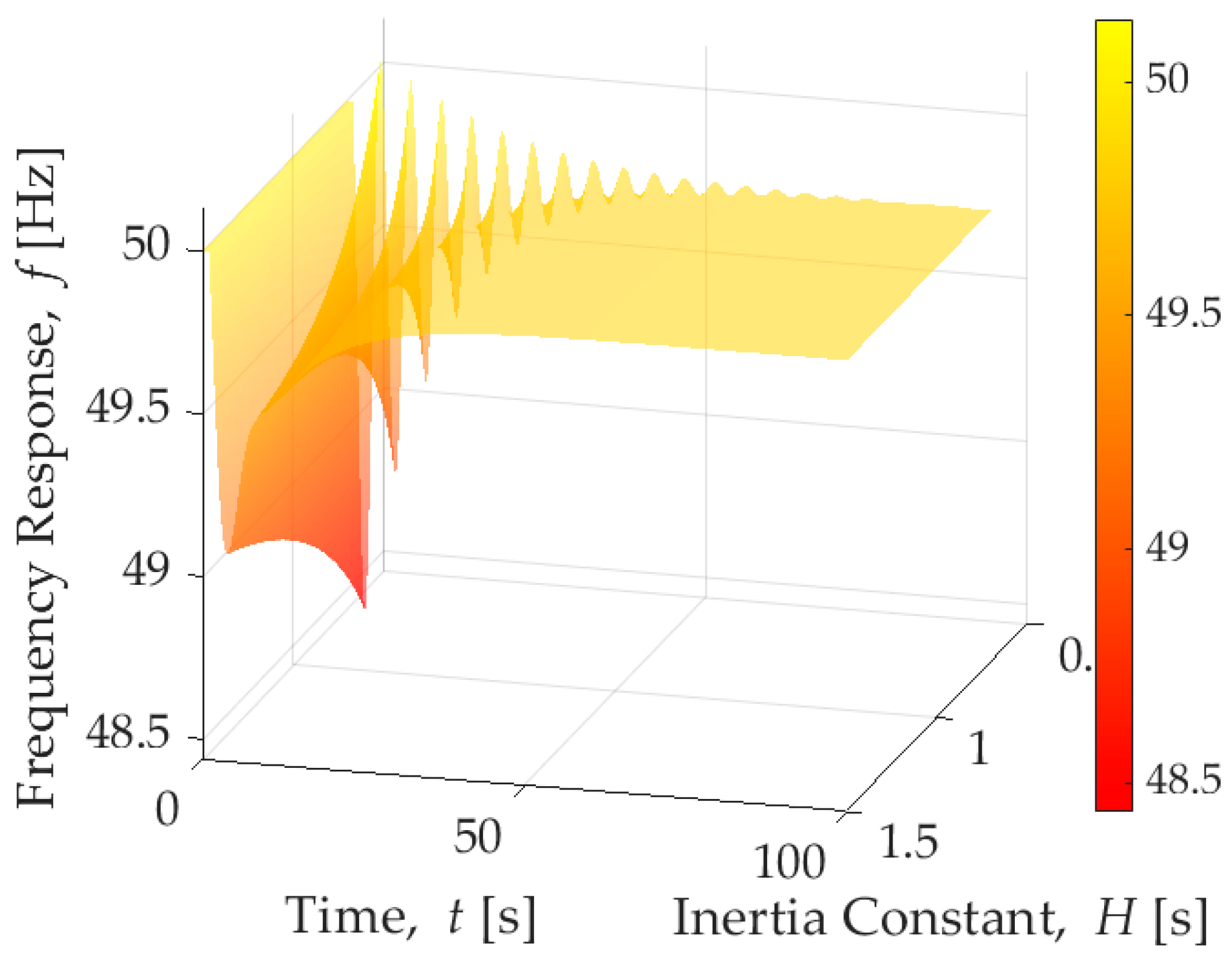
The effect in the system frequency response caused by the reduction of the total system rotational inertia of a simplified power system is shown in the form of the time-domain response of the frequency and
RoCoF,
Figure 4 and
Figure 5, respectively. The total system rotational inertia is reduced from the
Hhigh = 1.5 s to
Hload = 0.5 s considering changes of Δ
H = 0.025 s, for each change, a 100-s time-domain simulation is performed (total of 40 simulations).
The most obvious conclusion when looking at
Figure 4 and
Figure 5 is that the frequency goes deeper and faster as the rotational inertia is reduced.
Observing the system frequency response during the under frequency event as presented in
Figure 4, there are effects in the frequency performance indicators: (i) the minimum frequency (
fmin =
fnadir) decreases as the rotational inertia; (ii) the time to reach the minimum frequency (
tmin) increases as the rotational inertia increases, (iii) as expected, the steady-state frequency (
fss) remains unchanged when inertia changes.
However, beyond the well-known frequency indicators already described, a very important aspect to notice is the shape of the frequency response during the under-frequency event. High rotational inertia values tend to produce a more damped frequency response when compared with the low rotational inertia. Frequency response in low row rotational inertia tends to make the system frequency response oscillate faster (low damped oscillations).
Therefore, a power system in low rotational inertia conditions requires more carefully designed control actions to maintain the system frequency inside acceptable values.
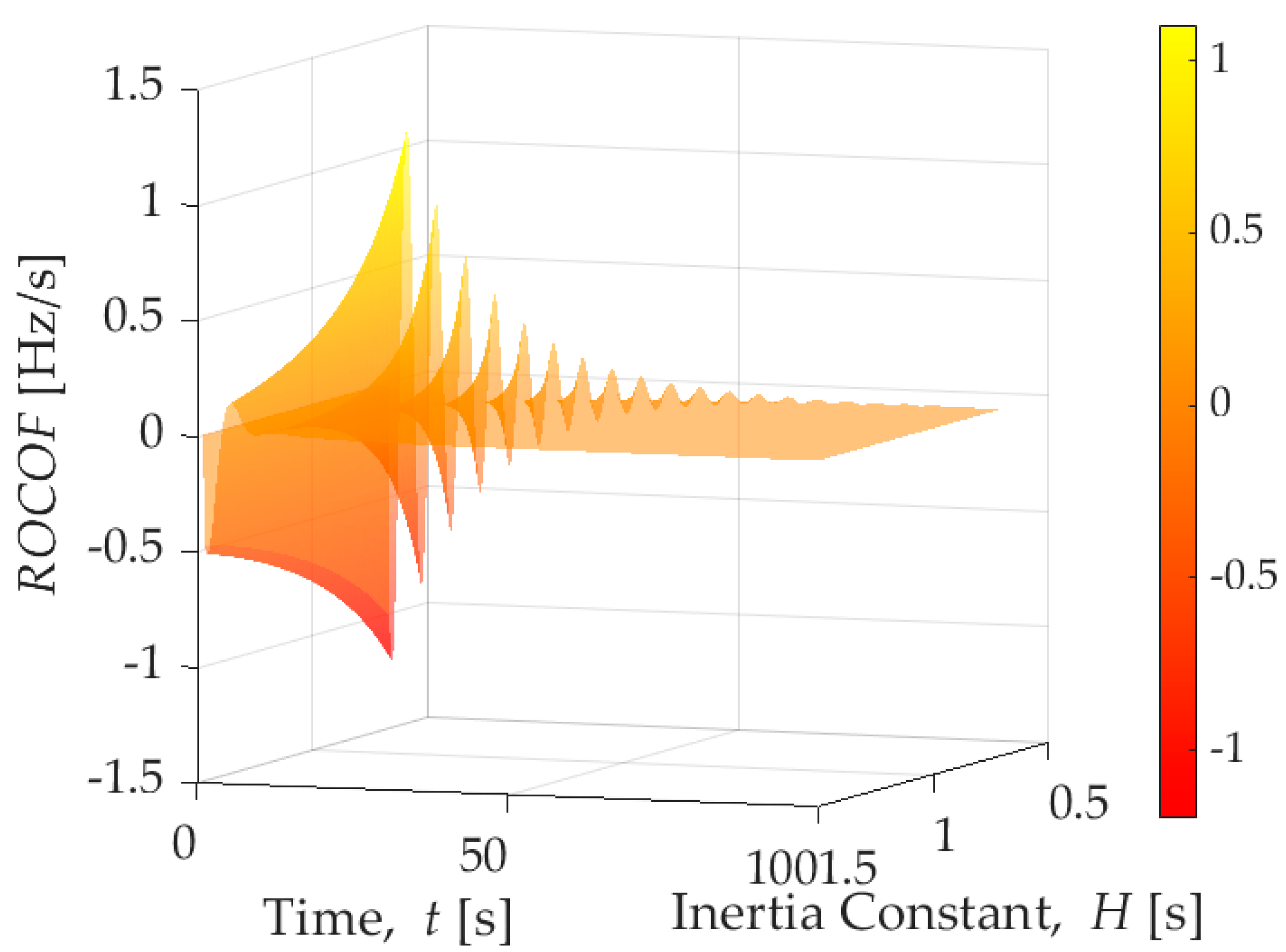
Figure 5 shows a very comprehensive plot of the
RoCoF experiences by the single area system (shown in
Figure 3); considering changes in the rotational inertia, operating conditions considering low rotational inertia produces higher values of
RoCoF when compared with the same at higher rotational inertia. However, the shape of the
RoCoF dynamic special attention deserves: high rotational inertia tends to exhibit an overdamped response, but as the rotational inertia decreases, the ROFOF exhibits an underdamped behaviour with an increase in the oscillation frequency and decreased damped.
4. Role of the Rotational Inertia in System Frequency Response
The system frequency of a traditional multi-machine power system is defined by the electromechanical dynamic of each synchronous generator directly connected to the system. The generator-demand electromechanical dynamic relationship between the incremental mismatch power (Δ
pi) and the frequency (
fi) can be expressed at
k–th generator using a simplified version of the so-called swing equation (neglecting all the damping effects):
where:
pmec,k represents the mechanical power of prime mover in pu,
pelec,k defines the electrical power in p.u., Δ
pk is the load generation imbalance in pu,
Hk indicates the inertia constant in secs,
fk is the frequency in Hz,
f0 is the rated frequency value in Hz, and
dfk/
dt is the frequency change in Hz/s. All those quantities represent the electromechanical variables of the
k-th synchronous generation unit of a total of
Ngen connected in the power system.
The frequency behaviour of a traditional power system during a system frequency disturbance using (1), if active power demand is greater than generation (
pelec,k >
pmec,k, Δ
pk < 0), the frequency falls (
dfk/
dt < 0) while if generation is greater than demand (
pelec,k <
pmec,k, Δ
pk > 0), the frequency rises (
dfk/
dt > 0). As the power system has
Ngen generation units, during an SFD each generator experiences a frequency dynamic described in (1), using the same approach used in classical mechanical systems, the concept of centre of mass can be invoked for the definition of a frequency of inertia centre (CoI). The frequency of CoI (
fCoI) represents the inertia-weighted average of all generator frequencies (
f1,
f2, …,
fNgen):
where
Htotal represents the total inertia of the system in sec (referred to the same base).
Considering a highly lossless meshed power system, all generation units can be assumed to be represented in a single busbar using the CoI of the system and, assuming further simplifications, they can even be condensed into one single equivalent unit. A summation of the non-linear differential Equation (1) for the case of
Ngen generators in the power system yields:
Assuming a strong coupling of the generation units following quantities can be defined:
During an SFR the system frequency (
fCoI) will change at a rate initially determined by the total system inertia (
Htotal). The contribution of the total system rotational inertia (
Htotal) of one rotational load or generator (
H) depends on if the system frequency causes a change in its rotational speed and, then, its
kinetic energy (
KE) [
35]. The inertia constant (
Hk) is a constant which has proved very useful. Considering real units, the inertia constant is defined as the kinetic energy (
KE) stored in the rotating masses (rotor) at rated speed (
ωsyn) divided by the rated apparent power of the machine (
G, MVA).
There are few interpretations of H, but if the units are appropriately selected, H represents the time in seconds a generator can provide rated power solely using the kinetic energy stored in the rotating mass.
The rotational inertia
H is of a synchronous generator defines the capability of the rotor of storing kinetic energy (
KE) in their rotating mass. This important electromechanical parameter depends on the total weight of the rotor, speed of rotation, and physical geometry of the rotor (diameter). The rotational inertia constant
H has the desirable property that its value, unlike those of inertia constant in mega-joule-seconds per electrical degree (
M) and moment of inertia (
WR2 in pound-feet
2), does not vary significantly with the rated kilovolt amperes and speed of the machine, but instead has a characteristic value of a set of values for each class of machine [
36]. In this respect, the rotational inertia
H is similar to the per-unit reactance of machines. It will be observed that the value of
H is considerably higher for steam turbogenerators than for water-wheel generators.
Rotational Inertia of Individual Generators
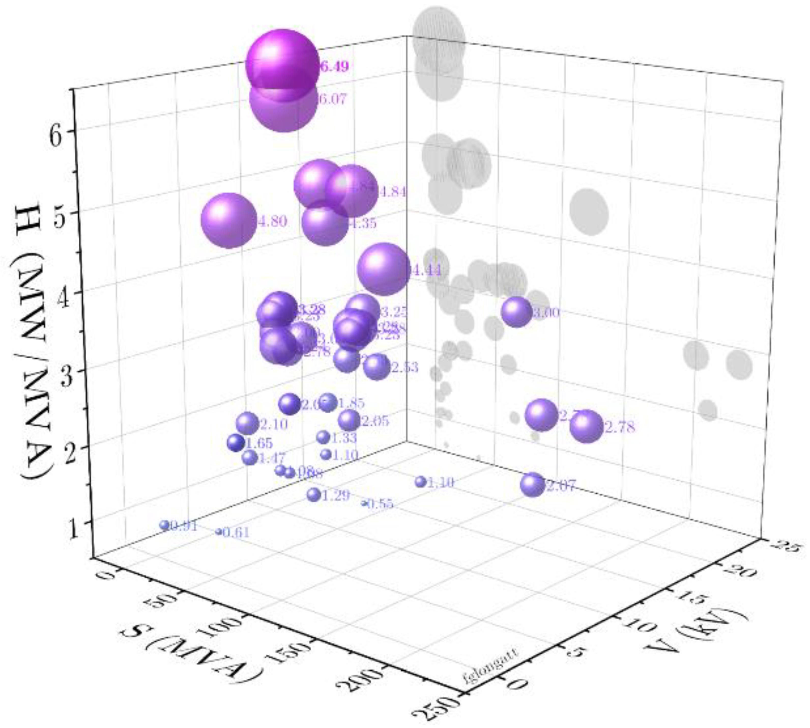
The following illustrates the variations of the rotational inertia between individual synchronous generators installed in a real power system, specifically, Chile and Peru in South America. Using publicly available data, a plot of the individual synchronous generator rotational inertia (
H in MW/MVA) versus rated apparent power (
Sn, MVA) and rated voltage (
Vn, kV) has been created for Chile and Peru,
Figure 6 and
Figure 7 respectively.
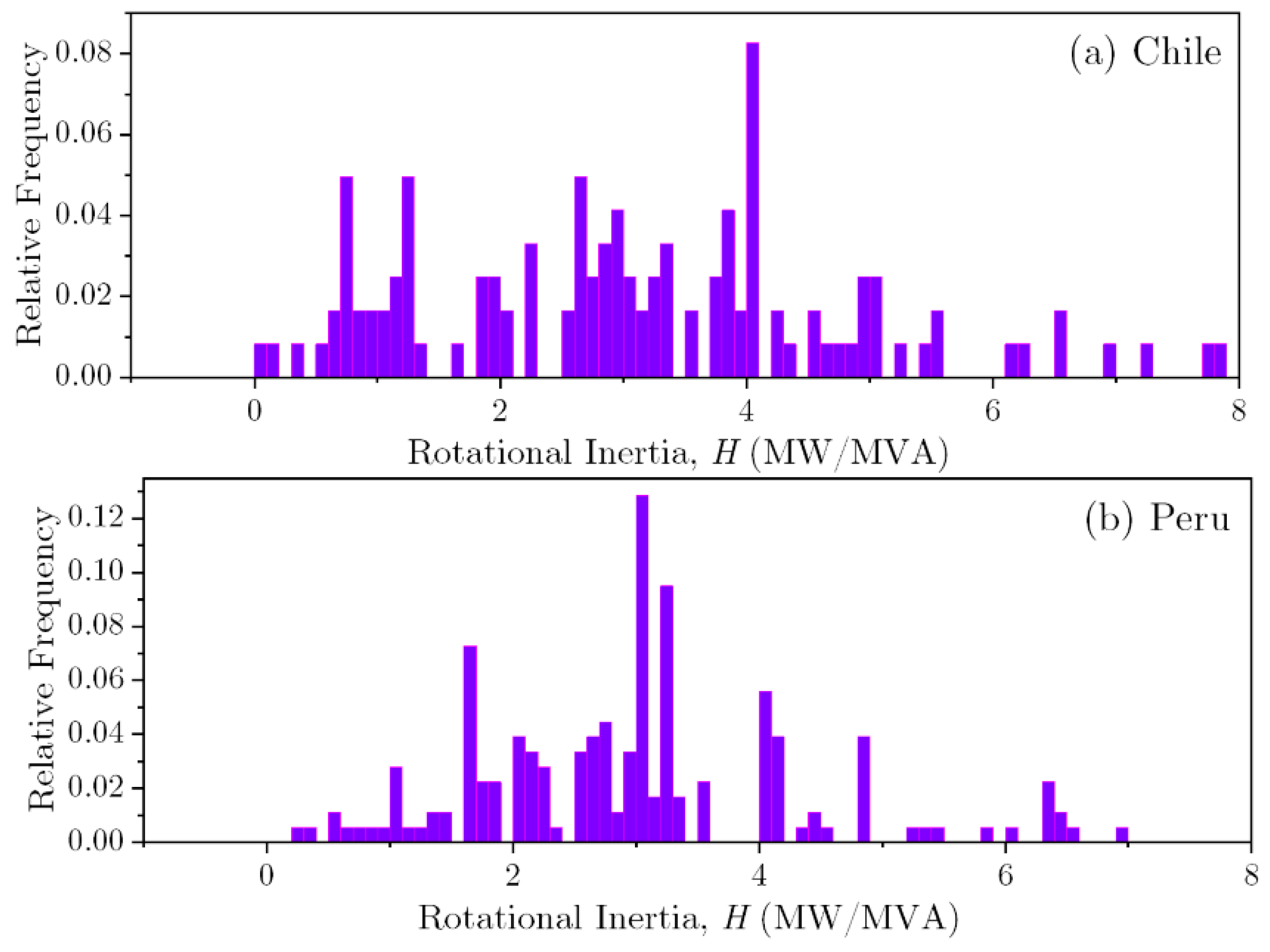
The Chilean power system has 25,000 MW installed capacity with around 26% of that coming from hydropower plants, a histogram of the rotational inertia of individual synchronous generators made clear the variation of its electromechanical property, the rotational inertia varies from 0.0495 MW/MVA to 7.8 MW/MVA (expressed in nameplate rate value) and averaging 3.0797 s. However, most rotational inertia is distributed between 2.0 and 4.0 MW/MVA (see
Figure 8a). On the other hand, the Peruvian power system has an installed capacity of 6000 MW, with 86.7% of the demand in the rural areas and thermal power plant generation representing the 52% of the installed capacity and 48% hydropower. The rotational inertia distribution of individual generators in Peru ranges from 0.2183 MW/MVA up to 6.9900 MW/MVA, and an average of 2.9689 MW/MVA. The relative frequency histogram of the rotational inertia shows a central tendency around 2.5 MW/MVA (see
Figure 8b). It is essential for the reader to understand that the previous analysis is related to the individual inertia of the installed generators, and it is not the total operating system available during the day a day operation of the system that depends on many other factors (operational and security constraints, etc.).
5. Inertial Response of Individual Generators
During a frequency event in a power system, the synchronous machine directly connected to the power system naturally and instantaneously will respond to the frequency variation [
30]. The electrical frequency variation is received by the synchronous machine as the frequency of the three-phase stator voltage signal changes. As the rotational velocity of the rotating magnetic field created by the stator departs from the synchronous speed, the electromagnetic torque between the rotor and stator tends to change, and at that moment, the moment inertia in the rotor tends to keep the rotational speed (Newton’s first law of motion), but a consequence is that the rotor will release/absorb kinetic energy.
The active power injection/absorption related to change in kinetic energy stored in the generator rotor is known as the inertial response. The inertial response (IR) of a synchronous generator following a power imbalance is mainly dominated during the initial stages by the frequency change (df/dt) or RoCoF (rate of change of frequency in Hz/s). The inertial response is a dominant dynamic process inherent to the synchronous generators directly connected to the power system; however, after a very short time where the kinetic energy is released, then the governor control has a dominant role in the electric frequency response.
It must be clear: the inertial response is related to the change in the active power of a synchronous machine (i.e., generator or synchronous capacitor) as a natural and spontaneous response to a change in the electrical frequency of the signals at the stator of the machine.
The inertial response is something natural in the synchronous machine; there is no need for measurements, processing, or control algorithm for this, on the contrary, the power electronic converters where the inertial response is enabled by control loops (a deeper discussion about this is beyond the scope of this paper).
As expected, the inertial response provided by a synchronous generator during a system frequency disturbance depends on many factors, but one of them is the value of the rotational of the generator.
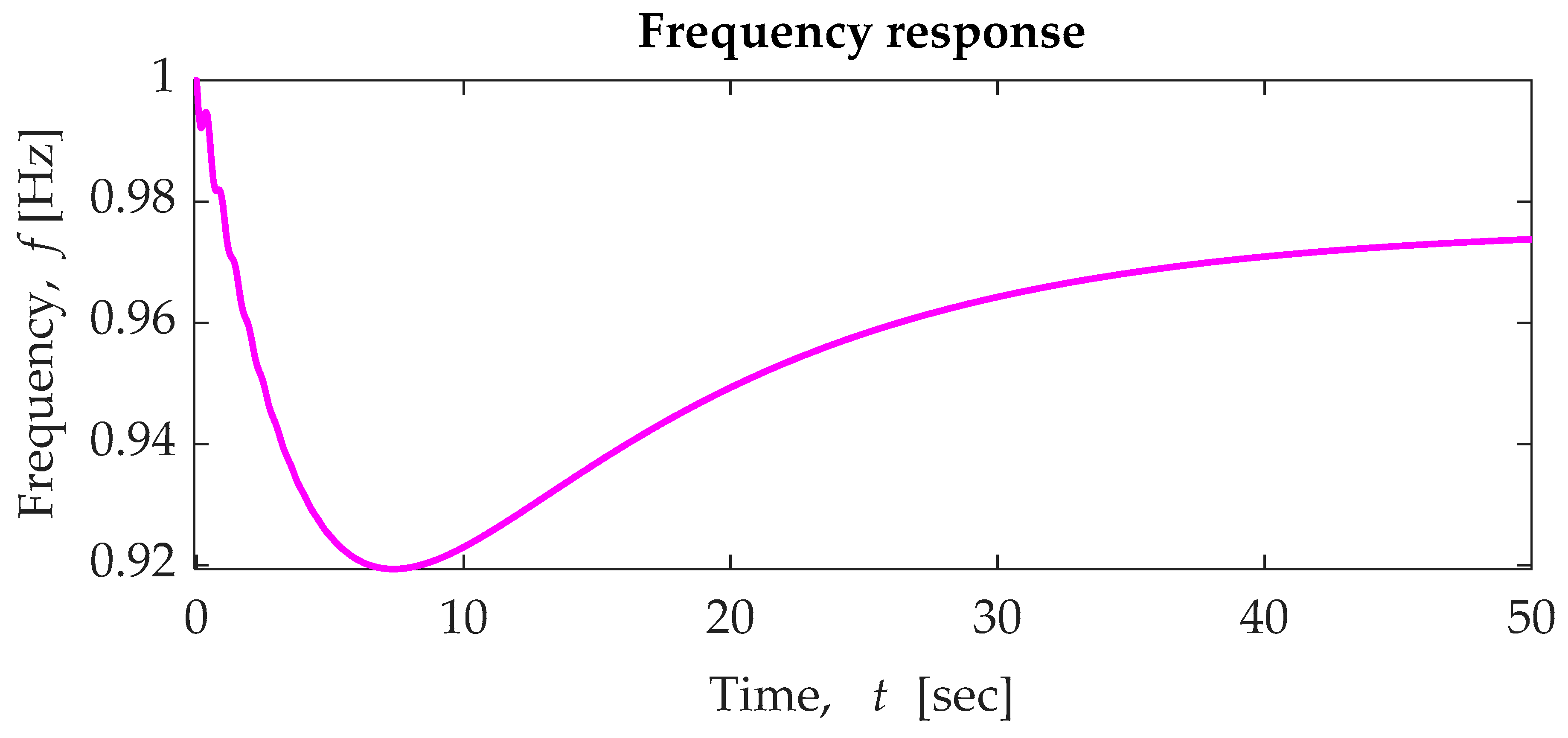
To illustrate the effect of the value of rotational inertia on the inertial response of a synchronous generator, a simple experiment is designed for that purpose. Consider a synchronous generator connected to a very large power system. To isolate the inertia response of the generator, it is assumed that the inertia constant of the total system is extremely large when compared with a synchronous generator, and then a system frequency event is applied. The event corresponds to an under frequency event as depicted in
Figure 9, the frequency drops at t = 0 to reach 0.92 pu at 8.67 s, and finally, the frequency reaches a steady-state frequency of 0.975 pu at 65 s (no shown in the plot below). The inertia response is evaluated to five (05) different synchronous generators; all of them are assumed to be synchronised and connected to the large power system and unloaded when the disturbance is applied; as this experiment is looking into the inertial response, the primary frequency response controller (e.g., the governor is not enabled).
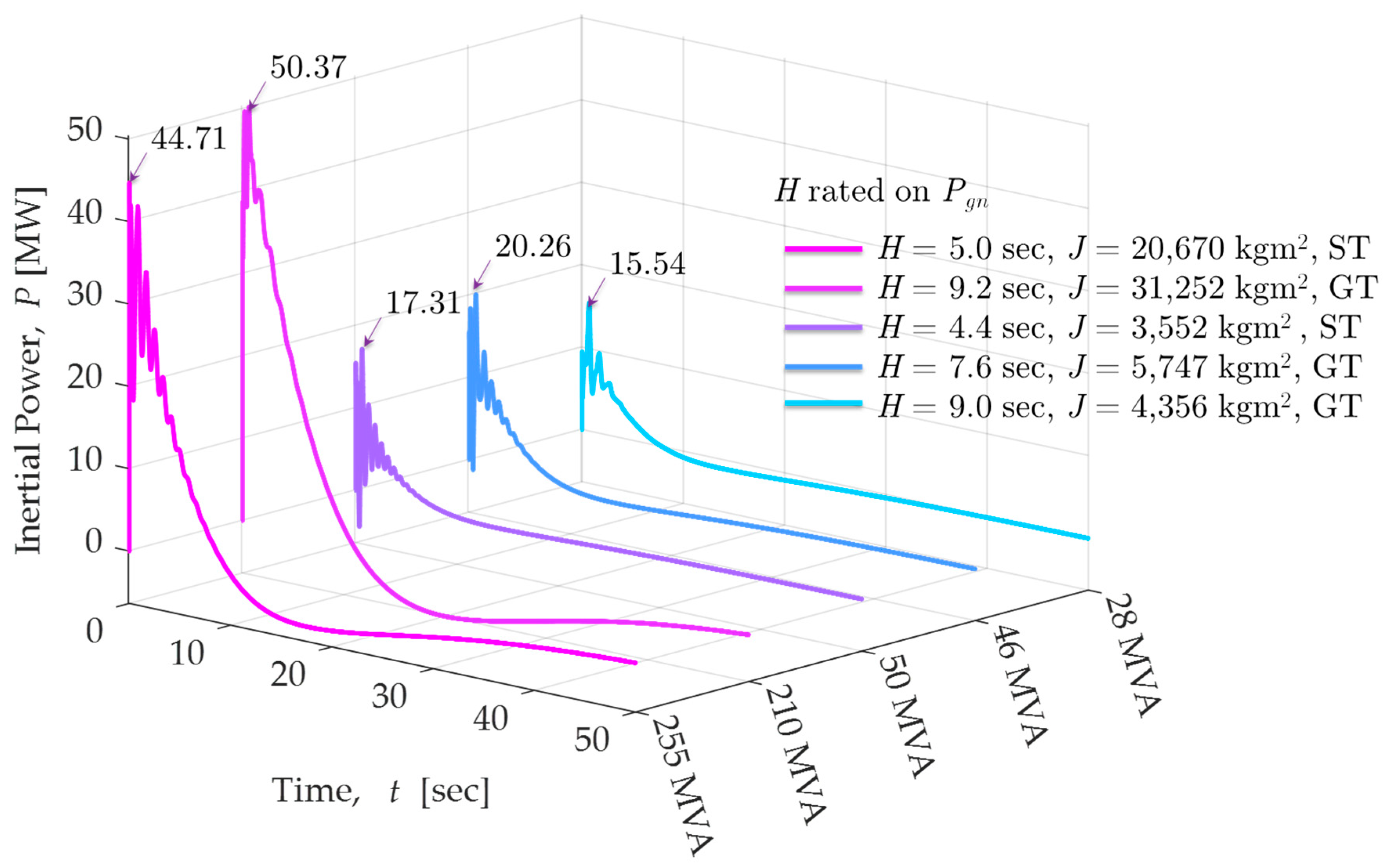
Five different synchronous generators are considered in the assessment, two of them low speed used at steam turbines (ST) and the remaining are typically found at gas turbines (GT); full details are shown in the embedded table in
Figure 10. The rotational inertia of those generators ranges from 4.4 s to 9.2 s, considering generation unit sizes from 28 MVA up to 255 MVA. Time-domain simulations are used to obtain the inertial response of each generator to the under frequency event, and time-series of the active power (also called inertial power) are presented in
Figure 10. It is clear that the larger the rotational inertia (
H), the higher the initial active power immediately after the disturbance (maximum 50.37 MW of 210 MVA, 9.2 s generation unit). Additionally, large rotational inertia implies more energy released during the frequency event.
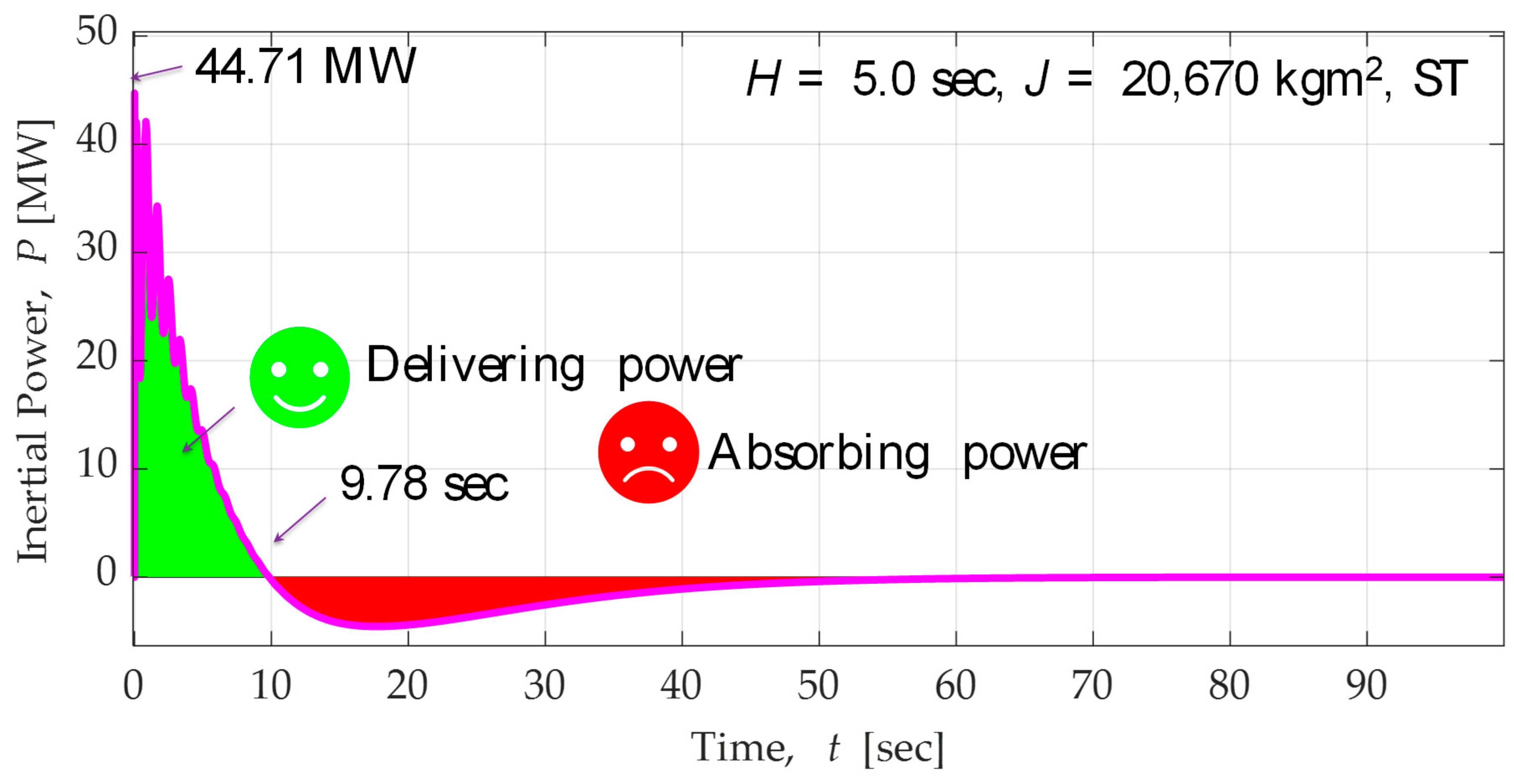
A very important aspect to discuss in relation to the inertial response of a synchronous machine is the implications related to the active power directionality and the energy involved in the process. As stated, before the synchronous generator will release energy as the frequency change, during that part of the process, the generator delivers extra active power, also known as inertial power.
Figure 11 shows the inertial response of the 255 MVA synchronous generator (
H = 5.0 s); the instantaneous inertial power reaches 44.71 MW immediately after the under frequency started. As depicted in
Figure 11, the inertial power is positive until 9.78 s after the disturbance indicating the generator is producing extra power (pre-contingency unloaded generator) and delivering energy to the large power system; the energy contribution is highlighted in bright green colour in the figure. However, after 9.78 s, the inertial power becomes negative and reaching −4.53 MW at 16.99 s; this situation represents the synchronous regenerator draining power from the large power system, and the total energy taken from the large power system is depicted in red colour.
The second part of the inertia response process (when the generators take power from the system) is a situation that is far from ideal. Looking into the frequency event (
Figure 9), the situation where the synchronous generator absorbs power from the grid happens during the under frequency event; consequently, there is a risk that the power abortion will recharge the rotational inertia can ignite a more severe under frequency event. In other words, it is far from ideal that a generator takes power from the large power system during the under frequency event, although this situation is solved in the traditional generation units by the inclusion of the primary frequency control-governor. However, the authors like to highlight this negative aspect of the recovery period of the inertial response as it must be taken into consideration when mimicking the inertial response of synchronous generator in control loops enabled in power electronic converters (further discussion is beyond the scope of this paper).
As stated before, the rotational inertia is located at the synchronous generator rotors, and they are spread throughout the electrical power system; during a frequency event, each synchronous machine directly connected to the power system will provide an inertial power contribution that depends on the rotational inertia and other factors (e.g., synchronising coefficients, etc.). During a power imbalance (independently of the size), the system’s frequency is not unique; in fact, each synchronous generator experiences changes in the rotational speed to accommodate the new operating status, and the frequency produced by each generator will be different. The frequency of the inertia centre (fCoI) as presented in (2) is a very important indicator used to assess the frequency response of a multi-machine power system; it represents an averaged frequency where the averaging weights are the rotational inertia of the synchronous generators involved in the frequency response.
To illustrate the role of the rotational inertia and the implications of the centre of in the system frequency response of a multi-machine power system, an experiment considering a three-control area power system is used.
Figure 12 shows the block diagram of one of the three identical interconnected control areas, and the complete set of parameters are shown in
Table 1.
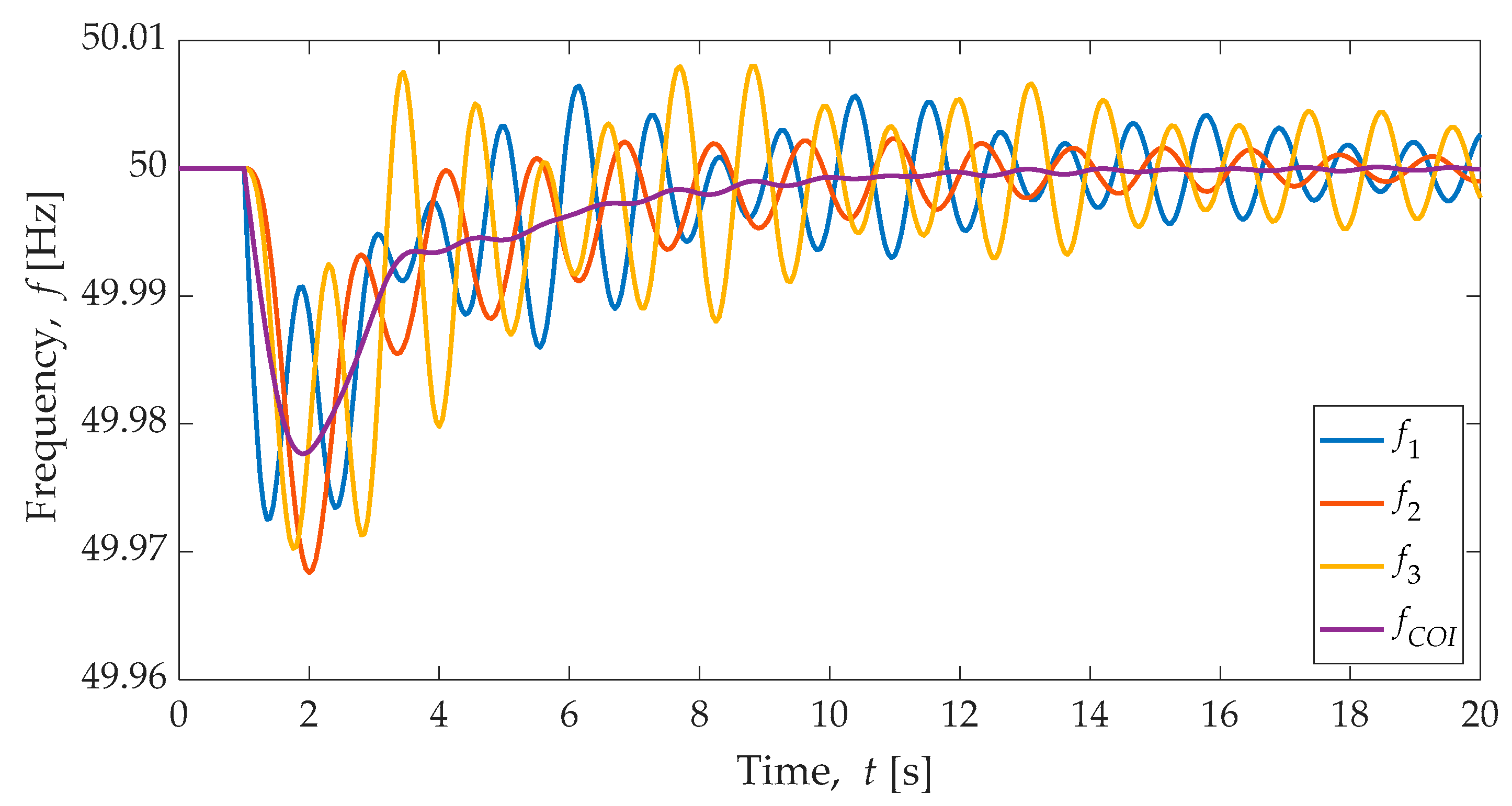
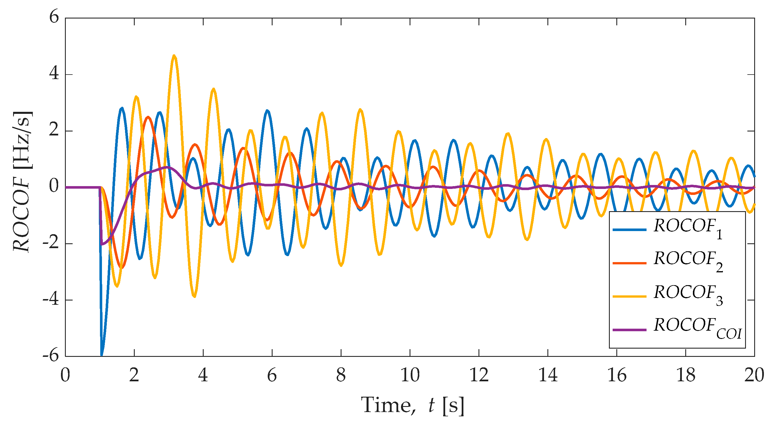
Figure 13 and
Figure 14 shows the plot of the frequency and
RoCoF behaviour during and under frequency event (sudden load increase, 20% in area 1 at
t = 1.00 s), the individual variables and the centre of inertia are depicted for illustrative purposes. As the system frequency disturbance happens in Area 1, it is clear the frequency of that area dropped the most and the fastest, Area 2 and Area 3 try to compensate for the power imbalance with inertial and governor response.
Observing the frequency response of the 3-area system, the nadir or minimum frequency occur at different times; specifically, the frequency response shows how Area 2 and Area 3 oscillate together as a group but against Area 1. The frequency of centre of inertia (fCoI) is used as a global indicator of the system frequency; during steady-state, all the synchronous machines rotate at the same speed (synchronous speed, ideally), and the frequency of the centre of inertia is equal to the frequency of each synchronous machine directly connected to the grid.
During an under frequency event, as shown in
Figure 13 and
Figure 14, the synchronous generators accelerate/decelerated depending on different speeds (depending on the inertia, instantaneous active power imbalance and governors characteristics), the frequency of centre of inertia represents and is averaged values of the frequency considering the individual inertias as a weighting factor. Although the main control and protection equipment are designed to operate based on local frequency, the frequency of inertia centre is used, typically, as a global indicator to assess the frequency response of a multi-machine power system.
This experiment demonstrates how the frequency in each control area might be different during the under-frequency event. However, the frequency of the centre of inertia can be used as an indicator when assessing the system frequency response of a system. However, it must be noticed that as a global indicator, the frequency of the centre of inertia tends to mask the local frequency variations.
6. Rate of Change of Frequency
This section is specifically dedicated to one crucial indicator of the system frequency response, the RoCoF. The frequency is a crucial electromechanical indicator that reflects the balance between generation and demand, and the derivate or rate of change has many applications. One of the most important uses of the RoCoF is as an indicator of frequency sensible protection relays. However, the recent interest of mimic the behaviour of synchronous machines by adding control loops to enable inertial response requires the RoCoF. This section is designed explicitly to shows one central aspect related to the RoCoF calculation in electrical power systems.
When the frequency is needed for monitoring, control, or protection purposes, it must be obtained using any calculation method. This process typically requires processing signals like instantaneous values obtained from voltage measurements. Many algorithms have been proposed in the scientific literature regarding the frequency estimation from alternating voltage signals [
28]: Phase Locked Loop (PLL), Fast Fourier transformation (FFT), Zero crossing of sinusoidal measurements, mainly busbar voltage used, Synchrophasor estimation, and derivation of angle. Other approaches based on parameter estimation or more complex techniques include [
28] Discrete Fourier Transform (and Kalman filtering), Taylor method, Shank method (LS), Kalman Taylor method (K), Wavelet, Least Squares Error, Least Means Squares, Kalman filters, or Newton-type etc.
The rate of change of frequency, also known as RoCoF, is a very important variable inside the power system operation and control; it can be used as an indicator for a protective function dedicated to fast load shedding. On the other hand, the RoCoF has an intrinsic relationship to the magnitude of the power imbalance during the frequency response; the RoCoF defines how quickly the generator speed changes and the system frequency changes. The RoCoF is expressed in Hertz per second (Hz/s); this might be used as a measure of the severity of a disturbance.
Considering the already presented swing equation, the most straightforward way to calculate the theoretical
RoCoF in single area power systems is considering the concept of centre of inertia; as a consequence, the
RoCoFCOI =
dfCOI/
dt immediately after a system frequency disturbance is calculated as:
where Δ
P represents the total power imbalance,
f0 is the system rated frequency,
dfCoI/
dt is the rate of change of frequency of the centre of inertia,
HT is the remaining rotational inertia constant of the entire power system after the disturbance, and
Sbase is the rated power of the power system (typically defined by the maximum expected peak demand). However, the calculation presented in the previous equation is possible when all the parameters are available and the variables are assumed continuous.
As explained before, the frequency is a variable typically obtained from processing the voltage signal and applying an estimation algorithm; consequently, the system frequency is typically available as discrete time series. Considering a discrete-time series of frequency measurements,
ft =
f(
t), where
t ∈ [
t0, …
tn], the most straightforward way to calculate the derivative of the frequency signal is by using the one-step incremental difference to approximate the derivative [
37]:
The approach presented above is mathematically correct but not realistic in practical terms. In real life, the majority of the operation and control applications use the so-called “moving window” or “rolling window”.
The
RoCoF calculation of an equally samples discrete time series can be represented by considering an
N-sample moving window [
37]:
where
Nsamples represents the number of samples in the moving window, one of the most exciting issues is related to the size of the moving windows. However, several transmission systems operators around the world have identified the size of the windows. There is no universally agreed value, and more critically, as the rotational inertia of the power system reduces, the calculation of
RoCoF must be calculated quickly to take decisions.
6.1. Effect of the Method and the Size of the Moving Window
This section explores the effect of the calculation method used and the size of the moving windows in the results of the
RoCoF. The method used to calculate
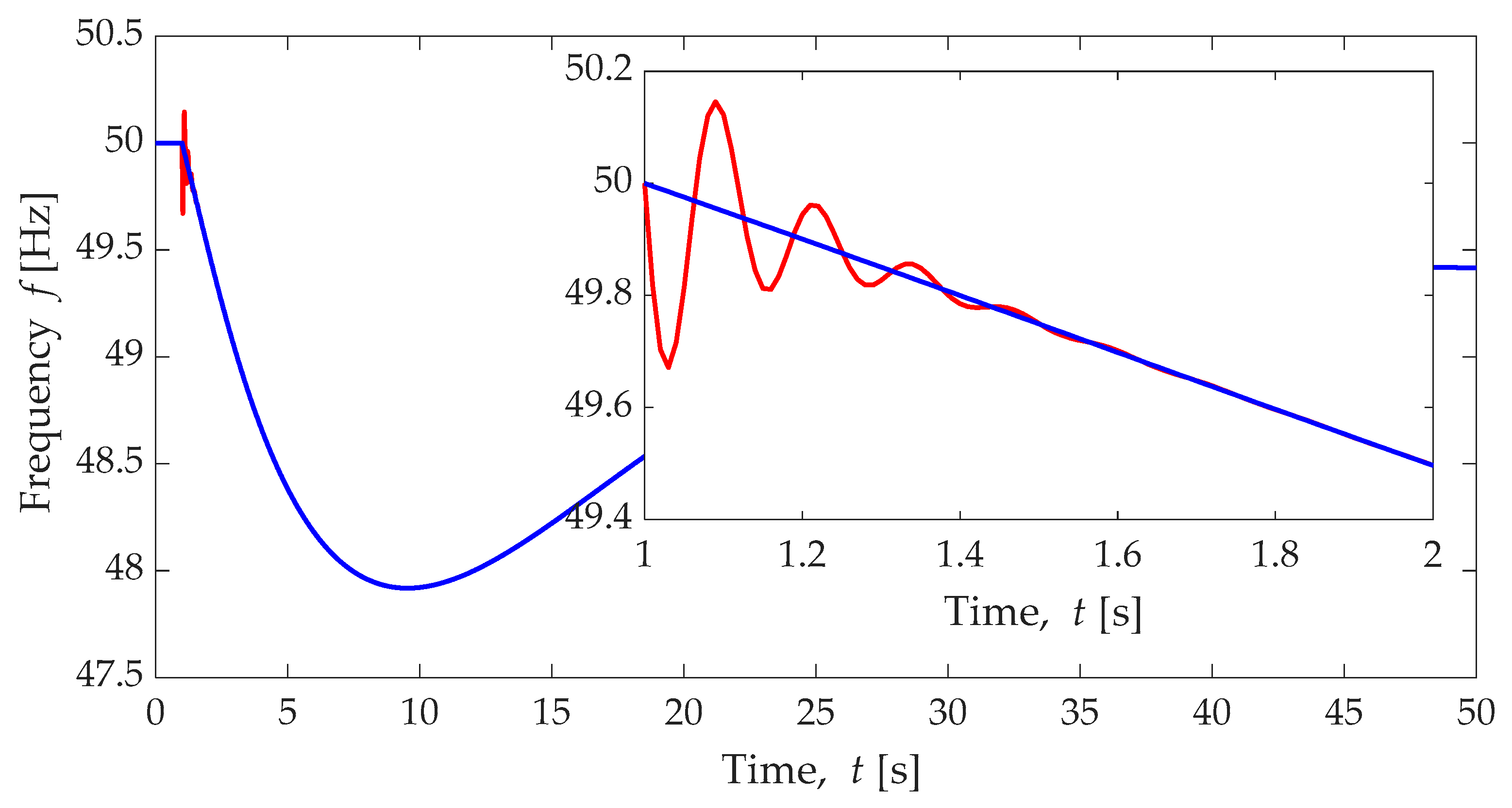
RoCoF has a remarkable effect on the instantaneous values calculated and used for operation and control and to illustrate that a simple experiment is used. Consider the system frequency response of a power system as shown in
Figure 15. The time series of the system frequency presented in
Figure 15 are created using power system analysis software. Two sampling frequencies are used to measure the system frequency: a high-speed sampling is able to record the high-speed transient inside the system frequency response of a single area power system (red colour plot in
Figure 15); when lower-frequency sampling is used, the transient is filtered (blue colour plot in
Figure 15), and it is clear the system frequency looks smooth.
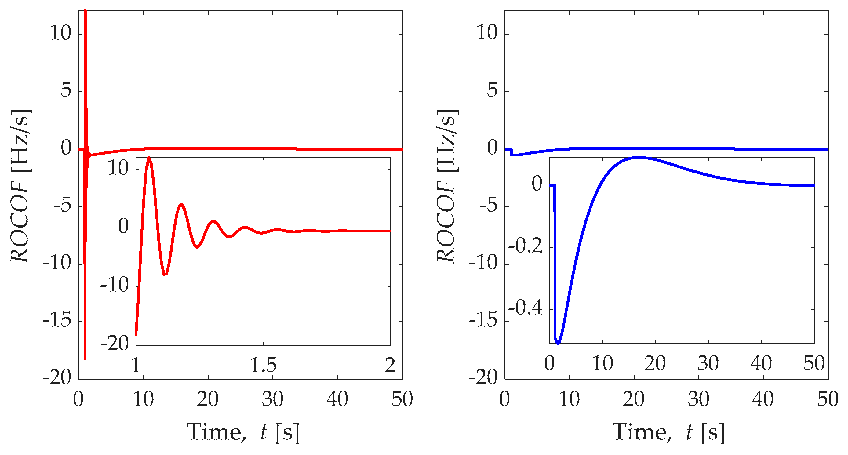
Considering the two sampled frequencies shown in
Figure 15, the
RoCoF is calculated by using one-step incremental difference, as shown in Equation (6), and results are shown in
Figure 16. Using the high sampling discrete frequency provides a higher instantaneous
RoCoF (~−18 Hz/s, left-hand plot in
Figure 16) and highly oscillating
RoCoF compared with the low sampling frequency (~−0.5 Hz/s).
Although the one-step incremental difference is a very straightforward calculation method of RoCoF, the reality is that using a single time step of the sampled frequency tends to amplify the noise, making this approach useless for real-life signals in noise environments. An extremely noisy RoCoF signal is not ideal if it will be used to emulate the inertial response in power electronic converters.
The European Network of Transmission System Operators for Electricity (ENT-SOE) has reported that a sliding window over approximately five consecutive measurements gives robust results. For the specific case of a 100 ms time resolution results in 0.5 s (500 ms) time is required before a reliable RoCoF value can be available.
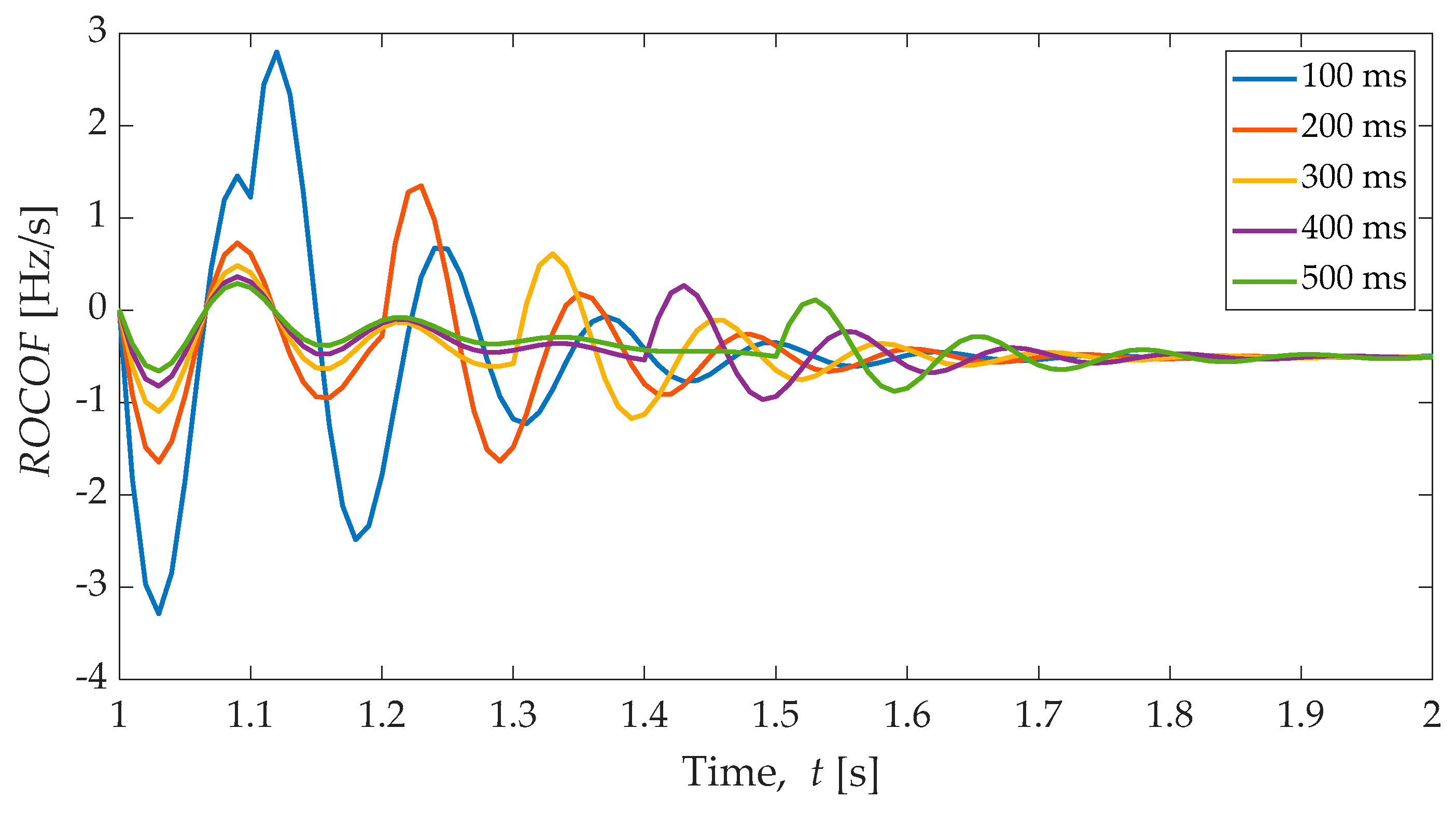
The frequency response (
f in Hertz) of a single area power system, considering high sampling frequency measurement (red colour in
Figure 15), has been used to calculate the
RoCoF, considering several windows size (from 100 ms to 500 ms), results are shown in
Figure 17. Large windows size tends to filter high-speed oscillations and displace the time of the maximum instantaneous
RoCoF.
The natural and pure electrical frequency created at the synchronous generators directly connected to the grid is a continuous variable typically smooth; however, as the frequency is typically obtained from processing the voltage signals, the sampling and processing process impact the frequency signal.
The previous experiment demonstrated the issues related to the method and the size of the moving window. Although the size of a window of 500 ms recommended in several places around the world, this experiment opens the door to considering the smallest moving window size; future scenarios of reduced rotational inertia in power systems will make the frequency moving faster and reaching even wider extremes, as a consequence, RoCoF is expected to increase and new approaches to accurately calculate the RoCoF must be evaluated.
6.2. Effect of Using Real Frequency Measurements
The previous subsection demonstrated that the size of the moving window has a significant impact on the RoCoF calculation; however, as classical control theory relates, the derivative control tends to amplify the noise of a signal. In the previous section, the experiment used time-series of frequency obtained from a digital simulation software; as a consequence, the problem of noise frequency signal and amplify noise in the RoCoF was not present. In this section, two experiments are presented to illustrate the issue of noise signals coming from real measurements and the amplification effect of the derivative calculation used to obtain the RoCoF.
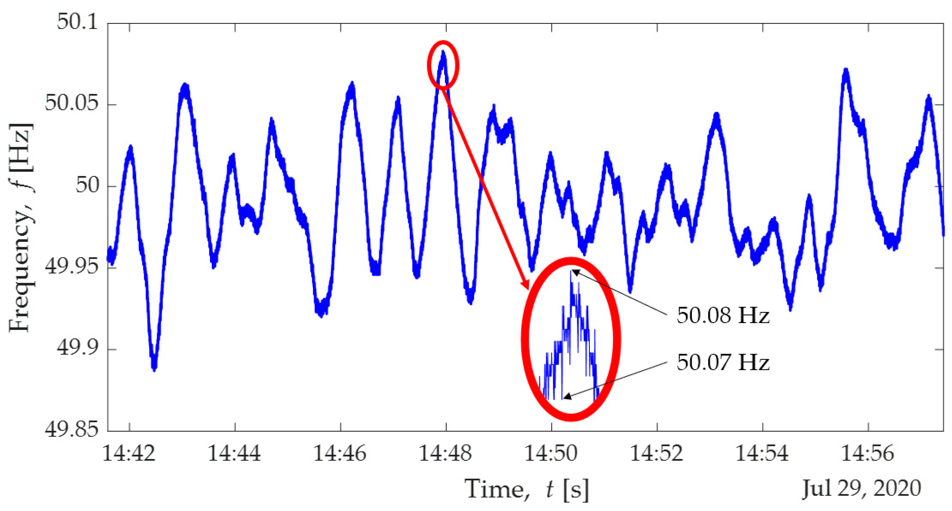
The experiment starts by collecting time series of frequency from a measurement device. The laboratory of Prof Gonzalez-Longatt (see
https://fglongattlab.fglongatt.org/index.html for more information, accessed on 6 September 2021) has a phasor measurement unit (PMU) Arbiter
TM Systems [
38] 1133A Power Sentinel
TM.The time-series of electrical frequency of the Nordic Power System was recorded using the Arbiter
TM Systems [
38] 1133A Power Sentinel
TM installed at Porsgrunn Norway (Lat 59°8′17.64″ N, Long 9°40′17.99″ E) and the time series is depicted in
Figure 18.
The Arbiter 1133A samples the voltages signals using a rate of 10,240 samples per second, considering a time stamp synchronised by a UTC-USNO (GNSS) within one microsecond [
39]. Fast Fourier transform (FFT) is used on the windowed voltage samples; the process is performed twenty times per second, using overlapping 1024-sample Hanning window data. The electrical frequency is measured by taking the difference in phase angle (
φ) between subsequent measurements (
φi−1 and
φi), based on the identity
f =
dφ =
dt. The frequency is averaged over one second prior to being displayed or made available for output [
39].
Figure 18 shows how the recorded electrical frequency varies over time; a simple zoom-in in the plot show how the signal has a small but high-resolution variability; this behaviour has a severe impact on the
RoCoF where the small changes in the measured frequency are significantly affected when moving window method is applied to the
RoCoF is used, this situation is depicted in
Figure 19.
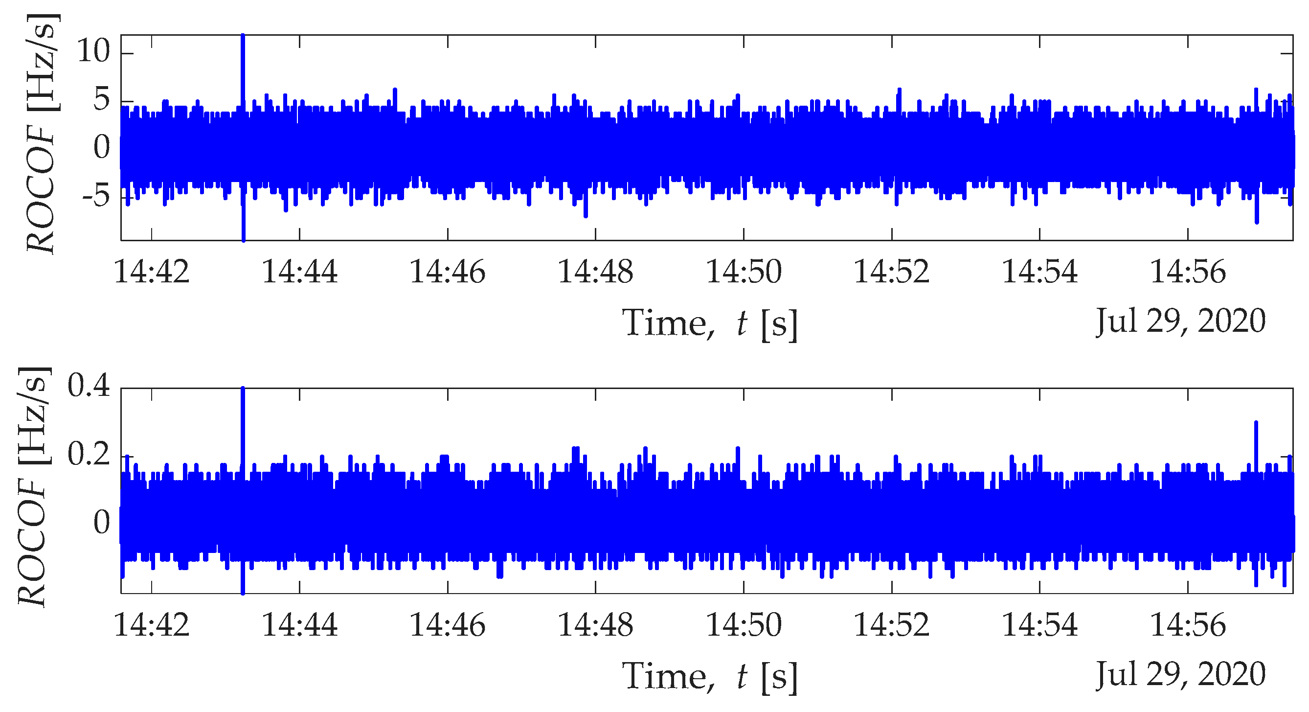
The recorded time series of the electrical frequency of the Nordic power system has been post-processed using a moving window to calculate the
RoCoF;
Figure 19 shows the results of using two different size windows, 0.04 s (top figure) and 500 ms (bottom figure). The time-series has been stored in a PC, and then a dedicated script was developed in MATLAB
® to calculate the
RoCoF using a moving window; this method is a very basic method, but it allows us to show the impact of the size of the window on the final
RoCoF. Comparing this with the plots at
Figure 19, it is clear that using a larger sample window (500 ms) tends to smooth at reducing the calculated
RoCoF (for this specific case 25 times less). However, this situation is like this because the moving window method is implemented in an ideal offline simulation environment.
RoCoF calculations implementation in real life has much more complex situations to tackle.
The RoCoF calculation in real environments is a much more complex process, the numerical results shown above are based on an electrical frequency time-series recorded in the Nordic Power system, and then RoCoF calculation is performed offline in a simulation environment. As a consequence, the calculation is performed without the issues related to the signal processing in real hardware. To illustrate the implications of using a frequency signal coming from a measurement and processing in a real hardware, a demonstrative experiment is used.


 ,
, 


