Can Deep Models Help a Robot to Tune Its Controller? A Step Closer to Self-Tuning Model Predictive Controllers

Abstract

Motivated by the difficulty roboticists experience while tuning model predictive controllers (MPCs), we present an automated weight set tuning framework in this work. The enticing feature of the proposed methodology is the active exploration approach that adopts the exploration–exploitation concept at its core. Essentially, it extends the trial-and-error method by benefiting from the retrospective knowledge gained in previous trials, thereby resulting in a faster tuning procedure. Moreover, the tuning framework adopts a deep neural network (DNN)-based robot model to conduct the trials during the simulation tuning phase. Thanks to its high fidelity dynamics representation, a seamless sim-to-real transition is demonstrated. We compare the proposed approach with the customary manual tuning procedure through a user study wherein the users inadvertently apply various tuning methodologies based on their progressive experience with the robot. The results manifest that the proposed methodology provides a safe and time-saving framework over the manual tuning of MPC by resulting in flight-worthy weights in less than half the time. Moreover, this is the first work that presents a complete tuning framework extending from robot modeling to directly obtaining the flight-worthy weight sets to the best of the authors’ knowledge.

1. Introduction

The model predictive controller (MPC) has shown remarkable success for the control and planning of numerous robotic systems [1,2,3,4,5,6,7,8,9,10,11,12,13,14]. However, its design necessitates an inevitable tuning procedure that involves the determination of its cost function weights. These weighting parameters essentially reflect the relative importance of each element in the underlying optimization problem. Traditionally, users prefer the trial-and-error method to obtain these weighting parameters either on a real robot or in simulation. Whereas the former might be dangerous—especially with aerial robots—the latter requires an accurate system model.

To mitigate the challenges faced by roboticists while tuning their MPCs, we present a novel, active exploration-based methodology. Rather than dispersedly exploring the viable weight set cluster via the trial-and-error approach, the proposed active exploration technique exploits the retrospective knowledge gained over previous trials and thus, efficiently tunes the weight sets. This is essentially achieved by adopting the exploration–exploitation concept of reinforcement learning (RL). Consequently, the auto-tuning mechanism significantly reduces the time and effort for MPC implementation and hence can be fairly useful for unskilled MPC users. This work is the first of its kind as being a complete tuning framework among a few other systematic MPC weight tuning guidelines in the literature. To list a few, [15] obtains some static tuning rules by first identifying the dominating tunable parameters and later analyzing their influence on the closed-loop MPC behavior. In [16], a simplified tuning expression is obtained for unconstrained linear MPC. In [17], a controller matching technique is utilized for selecting MPC weights. However, these approaches are restricted to linear systems. In [18], nonlinear process models are utilized for an offline, optimization-based tuning procedure for MPC. Nevertheless, this method requires a precise nonlinear model of the system. Additionally, an online, adaptive tuning strategy is proposed in [19], wherein analytical expressions for closed-loop response sensitivity to the tunable MPC parameters are obtained. Yet, this methodology may not be feasible for many robotic systems due to their complex, nonlinear dynamics.

Machine learning techniques are also incorporated for MPC tuning. As an extension to the work in [19], a fuzzy logic-based online tuning method for nonlinear MPC (NMPC) is proposed in [20]. The restricted gradient computation, which is required to determine the time propagation of the NMPC tuning parameters, is substituted by fuzzy logic. However, this method requires sufficient experience with the underlying system. Additionally, we would like to point out some RL-based (online) tuning of PID controllers from the literature [21,22,23,24]. However, in most of these implementations, the tuning starts from some precomputed gains via the Ziegler–Nichols (Z-N) strategy. Since the Z-N-like strategy is not available for MPC, the proposed active exploration approach obtains the flight-worthy MPC weight sets from scratch.

In the authors’ previous work [25], an RL-based automated (N)MPC tuning framework was developed and tested. The extensions and enhancements in this work over the previously published paper are threefold:

• Switching from the Gazebo model to the DNN model: previous work utilizes a Gazebo model of the robotic platform during weight set exploration. However, creating a Gazebo model requires expertise that may not be available for novice users. Hence, we opt for another simpler modeling approach in this work, i.e., deep neural networks (DNNs). Unlike the complicated process of obtaining a high-fidelity Gazebo model, in this case, novice users are only required to collect some data by manual flights and simply feed them to a DNN for modeling. Once trained, it will serve just like a Gazebo model to eliminate the need for risky trials on a real robot during weight set exploration.
• Fine-tuning of weight sets over real flights: to cater to several operational uncertainties, including decreasing battery voltage, communication delays, that may not be captured within the model, fine-tuning of the weight sets is also performed over the real robot. The real flight tuning feasibility of the proposed algorithm is demonstrated in this way.
• User study to evaluate the proposed tuning methodology: a comparison with the manual tuning procedure through a user-based study is performed, wherein users implicitly apply various strategies during the tuning process. Naively, they start by recognizing the dominating parameters and their effect on the performance, followed by the appropriate weight set selection. In essence, they optimize performance by exploring the selection space in a Bayesian way.

Moreover, the efficacy of the obtained weight sets for real-world applications is validated by extensive trajectory tracking results. Unlike the existing tuning guidelines in the literature, this work provides a complete tuning framework that begins with the robot modeling and, finally, results in the real flight-worthy weight sets. Additionally, the proposed auto-tuning framework is platform-independent and can be likewise implemented on any robotic platform.

This work is organized as follows: Section 2 introduces the utilized robotic platform. Section 3 illustrates the NMPC problem formulation. Section 4 presents the proposed tuning approach. Section 5 discusses the implementation results of the proposed method. Section 6 validates the applicability of the explored MPC weight sets in real flights. Lastly, Section 7 draws some conclusions from this work.

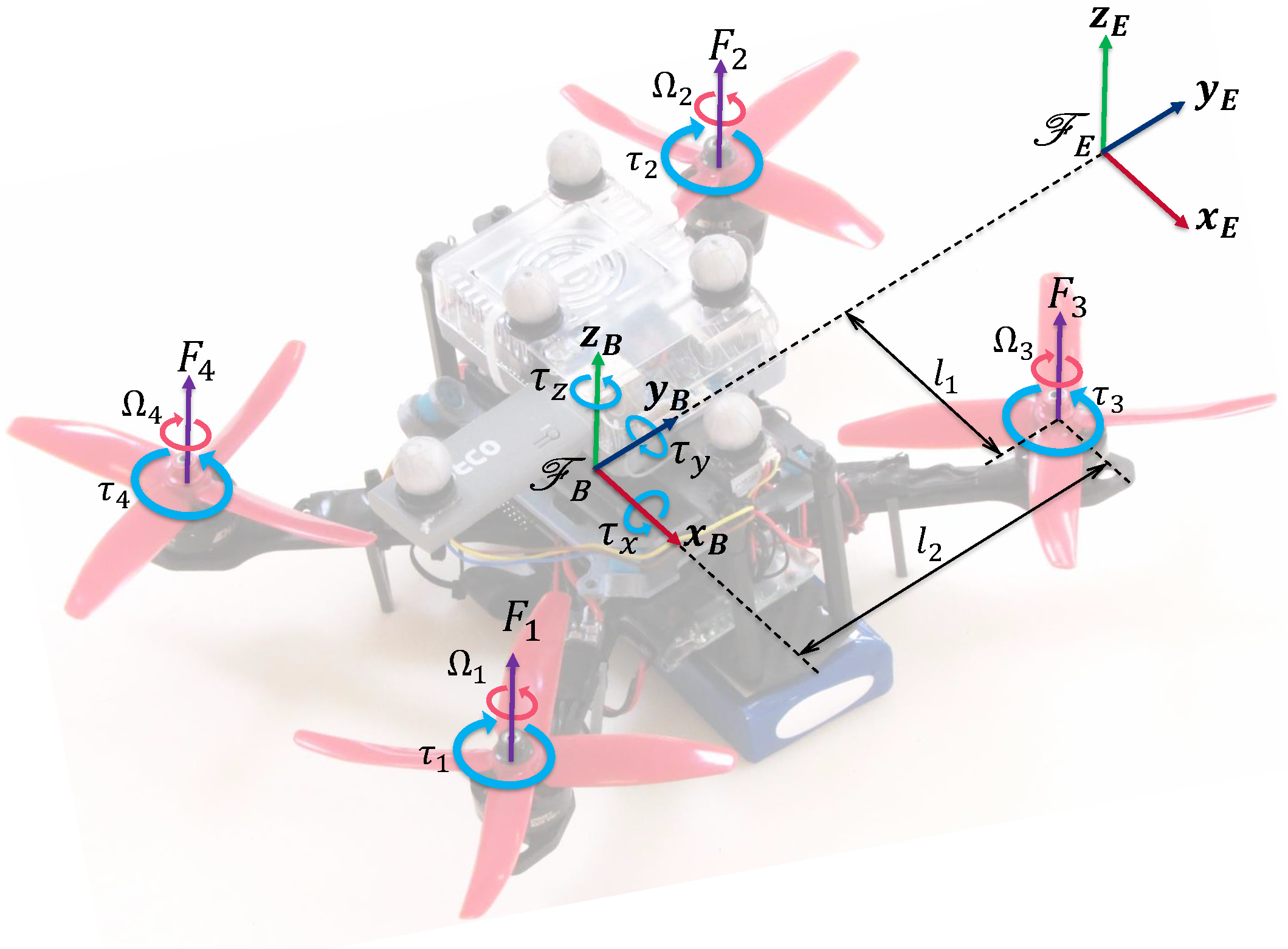
2. Quadrotor Aerial Robot

In this work, we utilize a micro-scale quadrotor robotic platform with “x-configuration” having arm lengths $l_1=0.073$ m and $l_2=0.098$ m, as displayed in Figure 1. The overall frame comprises of off-the-shelf carbon fiber arms that are assembled in-house. A Pixhawk flight controller is utilized for the low-level stabilization control, whereas an Odroid XU4 computer executes all the control codes onboard. The total takeoff mass (m) including all the onboard electronics is equal to $0.89$ kg.

The translational kinematics are obtained using the transformation from body frame (${\mathcal{F}}_B$) to Earth-fixed frame (${\mathcal{F}}_E$) as follows:

$$\left[\begin{array}{c}\dot{x}\hfill \\ \dot{y}\hfill \\ \dot{z}\hfill \end{array}\right]=R_{EB}\left[\begin{array}{c}u\\ v\\ w\end{array}\right],$$

(1)

where x, y, z represent the translational position which is defined in frame ${\mathcal{F}}_E$; u, v, w are the translational velocities that are defined in frame ${\mathcal{F}}_B$; $R_{EB}$ is the translation transformation matrix between frames ${\mathcal{F}}_E$ and ${\mathcal{F}}_B$, and is expressed as ($c:cos,s:sin,t:tan$):

$$R_{EB}=\left[\begin{array}{ccc}c\theta c\psi & s\varphi s\theta c\psi -s\psi c\varphi & c\varphi s\theta c\psi +s\varphi s\psi \\ c\theta s\psi & s\varphi s\theta s\psi +c\psi c\varphi & c\varphi s\theta s\psi -s\varphi c\psi \\ -s\theta & s\varphi c\theta & c\varphi c\theta \end{array}\right],$$

(2)

where $\varphi$, $\theta$, $\psi$ represent rotational attitude of the quadrotor defined in frame ${\mathcal{F}}_E$. On the other hand, the rigid-body dynamic equations are derived based on the Newton–Euler formulation in the body coordinate system. The quadrotor is assumed to be a point mass, wherein all the forces act at the CG [26]:

$$\begin{array}{}\mathrm{(3a)}& \dot{u}=rv-qw+g\sin (\theta )+\frac{1}{m}{F}_x,\mathrm{(3b)}& \dot{v}=pw-ru-g\sin (\varphi )\cos (\theta )+\frac{1}{m}{F}_y,\mathrm{(3c)}& \dot{w}=qu-pv-g\cos (\varphi )\cos (\theta )+\frac{1}{m}{F}_z,\end{array}$$

where $F_x$, $F_y$, $F_z$ are the total external forces acting on the quadrotor body in frame ${\mathcal{F}}_B$.

Finally, the lumped nonlinear dynamic model of the aerial robot at a high level can be written in a discretized form as:

$$\begin{array}{c}\hfill {\mathtt{x}}_{k+1}={\mathtt{f}}_{\mathtt{d}}({\mathtt{x}}_k,{\mathtt{u}}_k),{\mathtt{z}}_k=\mathtt{h}({\mathtt{x}}_k,{\mathtt{u}}_k),\end{array}$$

(4)

where $\mathtt{x}\in {\mathbb{R}}^6$, $\mathtt{u}\in {\mathbb{R}}^4$, and $\mathtt{z}\in {\mathbb{R}}^6$ are the state, control, and measurement vectors. For the considered quadrotor, state vector $\mathtt{x}$ and control vector $\mathtt{u}$ are comprised of:

$$\mathtt{x}={[x,y,z,u,v,w]}^T,\mathtt{u}={[\varphi ,\theta ,\psi ,F_z]}^T,$$

(5)

wherein the term $F_z$ in control vector is considered as the throttle command. The state and measurement functions are denoted by ${\mathtt{f}}_{\mathtt{d}}(·,·)$: ${\mathbb{R}}^6\times {\mathbb{R}}^4⟶{\mathbb{R}}^6$ and $\mathtt{h}(·,·)$: ${\mathbb{R}}^6\times {\mathbb{R}}^4⟶{\mathbb{R}}^6$, respectively.

3. Position Tracking Nonlinear Model Predictive Controller

In this work, an NMPC is designed as a high-level position controller. Its optimal control problem over a given prediction horizon ($N_c$) is defined in the form of a least-square function as follows:

$$\begin{gathered} \begin{array}{}\mathrm{(6a)}\underset{{\mathtt{x}}_k,{\mathtt{u}}_k}{\min }& \frac{1}{2}\{{\displaystyle \sum _{k=j}^{j+N_c-1}}\left({∥{\mathtt{x}}_k-{\mathtt{x}}_k^{\mathrm{ref}}∥}_{W_{\mathtt{x}}}^2+{∥{\mathtt{u}}_k-{\mathtt{u}}_k^{\mathrm{ref}}∥}_{W_{\mathtt{u}}}^2\right)+ \\ \left.{∥x_{N_c}-x_{N_c}^{\mathrm{ref}}∥}_{W_{N_c}}^2\right\}\mathrm{(6b)}& \mathrm{s}.\mathrm{t}.& {\mathtt{x}}_j={\widehat{\mathtt{x}}}_j,\mathrm{(6c)}& & {\mathtt{x}}_{k+1}={\mathtt{f}}_{\mathtt{d}}({\mathtt{x}}_k,{\mathtt{u}}_k),k=j,\cdots ,j+N_c-1,\hfill \mathrm{(6d)}& \hfill & {\mathtt{x}}_{k,\min }\le {\mathtt{x}}_k\le {\mathtt{x}}_{k,\max },k=j,\cdots ,j+N_c,\hfill \mathrm{(6e)}& \hfill & {\mathtt{u}}_{k,\min }\le {\mathtt{u}}_k\le {\mathtt{u}}_{k,\max },k=j,\cdots ,j+N_c-1,\hfill \end{array} \end{gathered}$$

where ${\widehat{\mathtt{x}}}_j\in {\mathbb{R}}^6$ is the current state estimate; ${\mathtt{x}}_k^{\mathrm{ref}}$ and ${\mathtt{u}}_k^{\mathrm{ref}}$ represent the state and control references; terminal state reference is given by ${\mathtt{x}}_{N_c}^{\mathrm{ref}}$; $W_{\mathtt{x}}\in {\mathbb{R}}^{6\times 6}$, $W_{\mathtt{u}}\in {\mathbb{R}}^{4\times 4}$, and $W_{N_c}\in {\mathbb{R}}^{6\times 6}$ are the corresponding positive (semi)-definite diagonal weight matrices which need to be tuned. The terms ${\mathtt{x}}_{k,\min }\le {\mathtt{x}}_{k,\max }\in {\mathbb{R}}^6$ and ${\mathtt{u}}_{k,\min }\le {\mathtt{u}}_{k,\max }\in {\mathbb{R}}^4$, specify the lower and upper bounds on the states and control inputs, respectively. It is to be noted that the high-level model in (6c), utilized in NMPC design is the first principle model as depicted in Section 2.

For our trajectory tracking application, the state, control, and measurement vectors for the position tracking NMPC are composed of:

$$\begin{array}{c}\hfill \begin{array}{cc}\hfill {\mathtt{x}}_{\mathrm{NMPC}}& ={[x,y,z,u,v,w]}^T,{\mathtt{u}}_{\mathrm{NMPC}}={[\varphi ,\theta ,\psi ,F_z]}^T,\hfill \\ \hfill {\mathtt{z}}_{\mathrm{NMPC}}& ={\mathtt{x}}_{\mathrm{NMPC}},\hfill \end{array}\end{array}$$

while the following state and control trajectories are given as references for the optimization problem:

$${\mathtt{x}}^{\mathrm{ref}}={\left[x_r,y_r,z_r,u_r,v_r,w_r\right]}^T,{\mathtt{u}}^{\mathrm{ref}}={\left[0,0,0,1.2mg\right]}^T,$$

where $x_r$, $y_r$, $z_r$ and $u_r$, $v_r$, $w_r$ are the position and linear velocity references, respectively. The control inputs from NMPC are passed to the low-level controller as its desired setpoints. The low-level controller in Pixhawk employs standard proportional-integral-derivative (PID) controllers, which are designed individually for each axis with the control vector ${\mathtt{u}}_{\mathrm{PID}}={[{\Omega }_1,{\Omega }_2,{\Omega }_3,{\Omega }_4]}^T$. Note that ${\Omega }_i$ represents the angular velocity of the $i\mathrm{th}$ rotor. The overall control scheme is summarized in a block diagram shown in Figure 2. Additionally, the following constraints are defined in the optimization problem for stable behavior:

$$\begin{array}{cc}\hfill 0.5mg(\mathrm{N})\le & F_z\le 1.8mg(\mathrm{N}),\hfill \end{array}$$

(7a)

$$\begin{array}{cc}\hfill -35{(}^{\circ })\le & \varphi ,\theta \le 35{(}^{\circ }).\hfill \end{array}$$

(7b)

Within the optimization problem (Section 3), we tune the diagonal elements of state and control weighting matrices, represented as $W_{\mathtt{x}}$ and $W_{\mathtt{u}}$, respectively. These weighting matrices penalize the deviations of predicted state and control trajectories from their specified references. Moreover, we select the terminal weight matrix as: $W_{N_c}=1.3\times W_{\mathtt{x}}$ and the prediction window $N_c$ as 30 for stability reasons. Typically, the terminal weight matrix is weighted more in comparison to the weight matrix for states, wherein the underlying reason is to ensure the stability of the optimal control problem (OCP) [27].

Remark 1.

One may note that while the proposed tuning algorithm can be utilized to obtain the terminal weight matrix, we preselect it for simplicity.

In addition to numerous optimization solvers proposed in the literature, a genetic algorithm-based solver has been developed for real-time control of an autonomous vehicle in [28]. Even though it renders flexibility in defining the OCP, the convergence time appears to be slow for systems with fast dynamics such as aerial robots. Therefore, in this work, the optimization problem in (Section 3) is solved utilizing the direct multiple shooting method due to its several computational advantages over the other techniques. Subsequently, the resulting discretized OCP is reduced to a sequential quadratic program after linearization. Finally, with the help of the generalized Gauss–Newton method, the solution to the obtained SQP is computed. Moreover, the adopted GGN method is a tailored variant of the classical Newton method which is solved with the help of a special real-time iteration (RTI) scheme proposed in [29].

4. Proposed Auto-Tuning Approach

The proposed approach (Figure 2) brings together concepts from RL and conventional trial-and-error-based MPC tuning. The presented methodology can be viewed as an advanced version of a traditional trial-and-error-based tuning process. It enhances the baseline trial-and-error method in two key aspects: eliminating the need for numerous trials on a real robot by utilizing a DNN model of it, and expediting the tuning process by benefiting from the active exploration paradigm which is inspired from RL.

4.1. DNN-Based System Modeling

Before the MPC weight tuning process, we created a full-state DNN model of the robot which was utilized in the tuning trials. Note that one could also utilize a model obtained via the first principle approach or could use some realistic simulators such as Gazebo. However, obtaining an accurate model via these approaches requires expertise and involves repetitive trials. Hence, the main reason to adopt neural network-based modeling is the ease of obtaining a high-fidelity model without requiring much expertise with system dynamics. Additionally, many off-the-shelf machine learning libraries such as PyTorch, TensorFlow, and Keras have made the training of DNN models much like a plug-and-play task, whereby the default settings work in most of the applications.

To create the DNN model, the flight data were recorded at 50 Hz. Within these data, twelve states of the quadrotor and four control inputs of the high-level controller—roll, pitch, yaw angle, and thrust—for a finite duration in the past ($0.8$ s) are regarded as inputs, whereas the resultant states of the quadrotor at the current time instant are regarded as outputs. Using these input–output data, we trained a feedforward DNN with 5 hidden layers and 288 neurons. We trained this network using Adam optimizer [30] in PyTorch with default settings through 510,000 data samples over 6500 epochs. Since the data were obtained from the real robot over a variety of trajectories, resulting in persistent excitation, the DNN represents the real robot’s dynamics fairly well. In this way, we attempted to assure that all the MPC weight sets obtained over the DNN model are real flight-worthy. Moreover, we would like to emphasize that other networks could also be utilized here as the network architecture does not play a vital role for the proposed algorithm in this paper. Nevertheless, the adopted network architecture embodies feature extraction and decision-making paradigms and has been shown to work well in the authors’ previous work [31].

4.2. Active Exploration of Weight Sets

The obtained DNN model can be used for trial-and-error-based tuning. However, it might take a considerable amount of time and effort from the users to try different weight sets, observe their performance on the model, and tweak them till finding viable weight sets. Thus, we automate this process by benefiting from the active exploration paradigm which is inspired by the conventional RL technique [32].

In the proposed auto-tuning method (summarized in Algorithm 1), different weight sets are deployed by adopting the exploration–exploitation concept from RL. Exploration refers to deploying a random MPC weight set while exploitation represents deploying a similar one to the best MPC weight set obtained until the current trial. As such, the similarity within exploitation is governed by a parameter $\lambda$ which represents the neighborhood radius for a weighting parameter as a percentage of its magnitude. Moreover, the balance between exploration and exploitation is governed by another parameter $ϵ$. By employing exploitation in addition to exploration, we made use of the grades of the previously deployed weight sets to interpret their neighborhood in the search space. This strategy caters to a more efficient exploration of the search space and yields better MPC weight sets over a shorter duration, as validated in the next section.

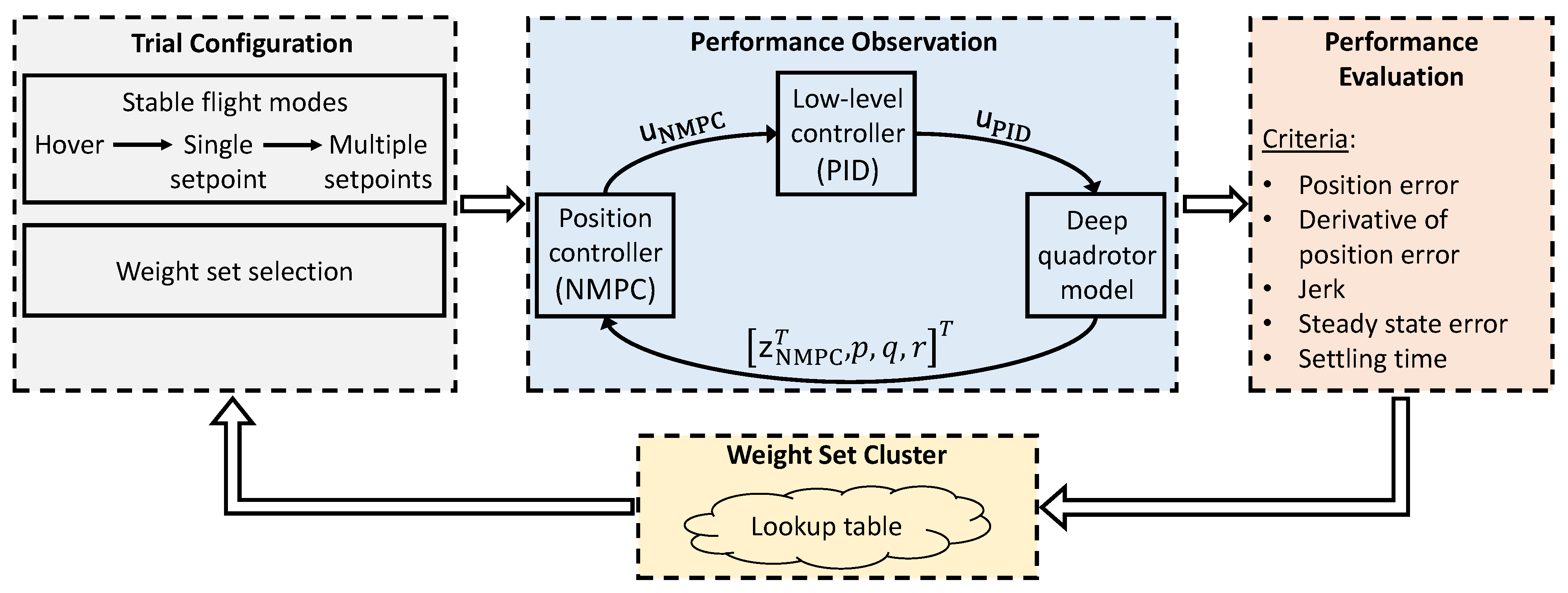
4.3. Overall Framework with Implementation Details

For the application in this work, we specify reasonable bounds to the search space as:

$$\begin{array}{c}\hfill \begin{array}{cc}\hfill & W_{\mathtt{x}}\in {\mathbb{W}}_{\mathtt{x}}=\mathrm{diag}({[\mathcal{O}({10}^2)]}^{1\times 3},{[\mathcal{O}({10}^1)]}^{1\times 3}),\hfill \\ \hfill & W_{\mathtt{u}}\in {\mathbb{W}}_{\mathtt{u}}=\mathrm{diag}({[\mathcal{O}({10}^2)]}^{1\times 3},\mathcal{O}({10}^{-2})),\hfill \end{array}\end{array}$$

(8)

where $\mathcal{O}$ represents the order of magnitude, and ${\mathbb{W}}_{\mathtt{x}}$ and ${\mathbb{W}}_{\mathtt{u}}$ are the corresponding search spaces in ${\mathbb{R}}^{++}$ (positive real values).

During auto-tuning, we considered three essential flight configurations which show the characteristics of common flight envelopes for quadrotors: “hover”, “move-to-a-setpoint”, and “follow-sequential-setpoints”. In hover mode, the robot tries to maintain its original position in the air. In move-to-a-setpoint mode, it tries to navigate to a predefined setpoint as fast as possible. In the aptly named follow-sequential-setpoints mode, the robot tracks a sequence of setpoints.

The criteria to assess different weight sets are position error (e), derivative of position error ($\dot{e}$), jerk (j), steady state error ($e_{ss}$), and settling time ($t_s$). After a flight trial, a weight set receives a sub-grade for each of these criteria by:

$$G_c=\left\{\begin{array}{cc}{G}_{c,max},\hfill & \mathrm{for}{G}_{c,max}\le G_c\hfill \\ \frac{c_{\mathrm{tol},\mathrm{init}}}{c},\hfill & \mathrm{for}c\le c_{tol}\hfill \\ -G_{c,max},\hfill & \mathrm{for}{c}_{\mathrm{tol}}<c,\hfill \end{array}\right.$$

(9)

where c is the corresponding criteria, $c_{\mathrm{tol},\mathrm{init}}$ and $c_{\mathrm{tol}}$ are the respective initial and current tolerance values for it. These sub-grades together form the grade G as follows:

$$G=\left\{\begin{array}{cc}\frac{1}{n}sum\left(G_e,G_e,G_j,G_{e_{ss}},G_{t_s}\right),\hfill & \mathrm{for}{G}_e,\cdots ,G_{t_s}\in {\mathbb{R}}^{+}\hfill \\ -G_{c,max},\hfill & \mathrm{otherwise},\hfill \end{array}\right.$$

(10)

where $n=13$ represents the number of criteria, $G_e$, $G_{\dot{e}}$, $G_j$, $G_{e_{ss}}$, $G_{t_s}$ represent the sub-grades, and $G_{c,\max }$ is the maximum sub-grade value which is set to 100 in this work. Moreover, the following expressions are defined for the weight set with maximum grade value in the lookup table:

$$W_{\mathrm{x},\mathrm{u}}^{*}=\left[W_{\mathrm{x}}^{*},W_{\mathrm{u}}^{*}\right]=\underset{W_{\mathrm{x}},W_{\mathrm{u}}}{max}G.$$

(11)

In addition, the relation between $c_{\mathrm{tol},\mathrm{init}}$ and $c_{\mathrm{tol}}$ is defined as:

$$c_{\mathrm{tol}}=\left(e^{-N_w/50}\right)c_{\mathrm{tol},\mathrm{init},}$$

(12)

where $N_w$ is the number of available weight sets with a positive grade in the lookup table. The motive behind this tolerance decaying approach is to always look for better weight sets that can satisfy stricter criteria. In this work, the initial parameters $c_{\mathrm{tol},\mathrm{init}}$ for the three different flight modes are selected as in

Table 1. Initial tolerance values for a stable flight.

Characteristics		Tolerance Values for Each Configuration
		Hover	Move-to-a-Setpoint	Follow-Sequential-Setpoints
Position error (m)	$e_x$	0.15	0.3	0.35
	$e_y$	0.15	0.3	0.35
	$e_z$	0.15	0.3	0.35
Derivative of position error (m/s)	$\dot{e_x}$	0.025	0.4	0.5
	$\dot{e_y}$	0.025	0.4	0.5
	$\dot{e_z}$	0.03	0.45	0.55
Jerk (m/s${}^3$)	$j_x$	0.5	2	2
	$j_y$	0.5	2	2
	$j_z$	1	3	3
Steady state error (m)	$e_{s{s}_x}$	0.15	0.15	0.15
	$e_{s{s}_y}$	0.15	0.15	0.15
	$e_{s{s}_z}$	0.15	0.15	0.15
Settling time (s)	$t_s$	1.5	4.5	4.5

, considering the usual values observed during common operations of quadrotors. However, since we incorporate exponential decay on $c_{\mathrm{tol},\mathrm{init}}$ as described in (12), the initial value selection is flexible as long as the values comply with safe flight conditions.

Algorithm 1 Auto-tuning approach

5. Tuning Approach in Action

In this section, we present the implementation results for the proposed active exploration-based tuning methodology. We first discuss each design setting over batched tuning sessions in simulation and then select the best setting which caters to our needs. Subsequently, we fine-tune the weight sets from simulation-based tuning in real flights. Note that, while the simulation tuning sessions are performed on a workstation computer with 2.6 GHz Intel Core i9-7980XE (octadeca-core) processor with 128 GB RAM, the real flight tuning is performed on a laptop having Intel Core i7-8750H processor and 16 GB RAM.

5.1. Benchmark Study for Simulation-Based Tuning

We conducted a benchmark study to justify our design choices for the proposed auto-tuning method. For each design choice, we conducted a batch of ten tuning sessions to obtain generalized results. We first examined a heuristic to expedite the tuning process, i.e., we assumed that the weighting parameters along the x- and y-body axes are close to each other since quadrotors are symmetrical with respect to these axes. Hence, we generate the respective weights in these axes within each other’s $10\%$ magnitude neighborhood. Without this heuristic, no positively graded weight set is explored in more than half of the sessions, even in the 1000 episode setting (

Table 2. Number of sessions without a positively graded weight set by using and omitting the heuristic.

Episodes	Without Heuristic	With Heuristic
100	10	7
500	7	2
1000	7	1

). By exploiting this heuristic, on the other hand, desirable weight sets were obtained in most of the sessions for 500 episodes and some of the sessions for even 100 episodes. Therefore, we employed this heuristic for the rest of the results presented in this work.

In

Table 3. Number of sessions without a positively graded weight set by active and random exploration.

Episodes	Active ($\mathit{ϵ}=0.5$)	Random ($\mathit{ϵ}=1$)
100	7	8
500	2	4
1000	1	1

, we present the numbers of sessions in which no positively graded weight set is explored. For both active ($ϵ=0.5$, $\lambda =20\%$) and random ($ϵ=1$) explorations, 100 episodes seem to be less to explore desirable weight sets. There are seven failed sessions out of ten sessions for active exploration in this case. For the 1000 episodes, on the other hand, there is only one failed session ($90\%$ success) both for active and random exploration. There are only two failed sessions when the episode number is 500, which implies $80\%$ success. We selected this setting for our tuning purpose since 1000 episodes take on average 2 h, which is more than twice the duration of 500 episodes (less than an hour), while the success rate improvement is only $10\%$.

Remark 2.

Probabilistically speaking, the notion behind selecting $ϵ=0.5$ is to realize equal occurrence for exploration and exploitation. In essence, it is a parameter that trades off the tuning speed with the exploration of the search space, thereby affecting the weight set quality. Note that owing to the high fidelity DNN model, users can set this parameter to a higher value for an optimal search of the weight set space, without having any safety concern for the robot. On the other hand, the selection of the similarity parameter $\lambda =20\%$ is essentially carried out via the trial-and-error method. During the trials, it has been inferred that setting a high value for this parameter facilitates a random selection which is contradictory to exploitation.

In

Table 4. Number of positively graded weight sets obtained by active and random exploration.

	Active ($\mathit{ϵ}=0.5$)		Random $(\mathit{ϵ}=1$)
Episodes	Average	Maximum	Average	Maximum
100	$1.4$	6	$0.2$	1
500	$12.7$	24	1	2
1000	$15.5$	23	$1.3$	3
Mean	$9.87$	$17.67$	$0.83$	2

, we present the average and maximum numbers of positively graded weight sets. The proposed active exploration outperforms the random exploration by yielding a higher number of positively graded weight sets. It obtains substantially more weight sets in a similar amount of time. A remark to be made here is that the number of weight sets obtained does not change significantly when the episode number is increased from 500 to 1000, while the overall tuning duration increases by approximately two times. This result further supports our previous episode number selection of 500 due to the trade-off between the tuning duration and success rate.

In

Table 5. Grade values for the positively graded weight sets by active and random exploration. One may notice the same average and maximum grades for $ϵ=1$ with 100 episodes. This is due to the single positively graded weight set as resulted by the corresponding setting (Table 4).

	Active ($\mathit{ϵ}=0.5$)		Random ($\mathit{ϵ}=1$)
Episodes	Average	Maximum	Average	Maximum
100	$10.52$	$10.76$	$7.18$	$7.18$
500	$9.08$	$10.21$	$8.64$	$9.21$
1000	$9.01$	$10.29$	$8.64$	$9.17$
Mean	$9.54$	$10.42$	$8.15$	$8.52$

, we present the average and maximum grade values for the positively graded weight sets obtained over ten sessions. In all the three episode-number settings, average and maximum grade values are higher for active exploration. In other words, the weight sets obtained via active exploration satisfy stricter criteria (e, $\dot{e}$, j, $e_{ss}$, $t_s$), and hence, they are better in quality. All these results prove the superiority of the proposed tuning method over the random trial-and-error method.

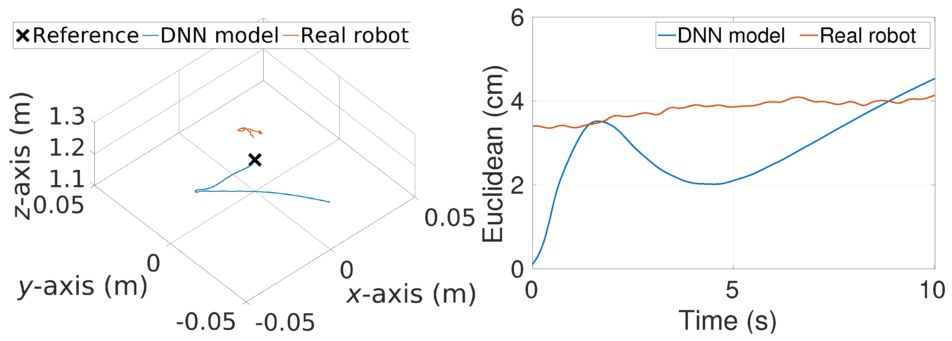
5.2. Further Tuning in Real Flights

Although the weight sets obtained over the DNN model are real flight-worthy, we investigate fine-tuning possibilities on these weight sets to achieve better flight performance. For fine-tuning in real flights, we first obtain new grade values for all the positively graded weight sets obtained in simulation-based tuning. This step is conducted to account for possible real-world operational uncertainties. As expected, only 17 out of 19 weight sets yield new grade values as positive. In other words, there are some weight sets, which can fulfill the design criteria (Table 1) over the DNN model but are unable to do so over the real robot. We then perform the real flight tuning over 30 episodes with $ϵ=0$ and $\lambda =10\%$ using the new grades. These hyperparameters are conservative versions of the ones selected for simulation-based tuning to account for safety. In essence, $ϵ=0$ makes sure that there will not be any trial with a random weight set on the real robot, i.e., no exploration. In addition, $\lambda =10\%$ focuses the search closer to the desirable weight sets, implying restricted exploitation. Throughout the real flight tuning, the average and maximum grade values increase from $9.34$ and $12.36$ to $9.68$ and $13.33$. This result demonstrates the successful fine-tuning in real flights.

Remark 3.

Note that the stochastic operational uncertainties would require an indefinite amount of data for training the DNN model. As such, one could decide to collect hours and hours of operational data for creating a highly accurate DNN model and just perform DNN-based MPC tuning. Another approach is to create a fairly accurate DNN model with a moderate amount of data and perform MPC tuning over it; followed by repeating the tuning procedure over the real robot to further improve the quality of the obtained weight sets. In this work, we utilize the latter, even though it is the user’s preference.

6. Trajectory Tracking

In this section, we present evaluative results for the weight sets obtained using the proposed auto-tuning method. We selected the weight set with the highest grade from simulation-based tuning and deployed it in the position tracking NMPC for tracking two types of trajectories: hover ($x=0$, $y=0$, $z=1.2$ m), and sequential setpoints (setpoints being $0.6$–$1.2$ m apart). We also utilize the weight set having the highest grade from real flight tuning for tracking the same trajectories. We then compare the performance of these two groups of weight sets to further justify the fine-tuning in real flights. Moreover, a demonstration Video S1 of this work can be found at: https://youtu.be/GLxRPCyNogc, (accessed on 4 September 2021).

6.1. Simulation-Based Tuning

The best weight set from simulation-based tuning is:

$$\begin{array}{c}\hfill \begin{array}{cc}\hfill W_{\mathtt{x}}^{*}& =\mathrm{diag}(16,11,13,2.0,2.1,2.3),\hfill \\ \hfill W_{\mathtt{u}}^{*}& =\mathrm{diag}(17,13,76,0.058).\hfill \end{array}\end{array}$$

(13)

For hovering, this weight set results in a precise tracking with mean Euclidean error values of 3–4 cm over both the DNN model and real robot, as visible in Figure 3. For the sequential setpoints tracking case, it again yields a precise tracking with mean Euclidean error values of 21 cm (Figure 4). A similar performance was obtained for the DNN model and real robot for both the trajectories, further validating the high fidelity of the DNN model.

Remark 4.

In Figure 4, one may note that the error values for sequential-setpoints are significantly higher as compared to the ones obtained for hovering (Figure 3). The main reason behind this is the underlying jumps of $1.2$ m that the robot has to execute to reach the commanded setpoint as fast as possible.

We repeat the above experiments with the ten best weight sets from simulation-based tuning to assess the overall quality. Their corresponding mean Euclidean error values are presented on the left side of Figure 5. The average and maximum error values over the DNN model are $2.98$ and $3.49$ cm for hovering. The same values over the real robot are $5.11$ and $7.94$ cm. A similar result is obtained for sequential setpoints. The respective average and maximum error values rise from $22.12$ and $26.61$ cm over the DNN model to $22.21$ and $28.27$ cm over the real robot. The slight error rise in the case of the real robot is mainly due to the operational uncertainties that are possibly not captured by the DNN model.

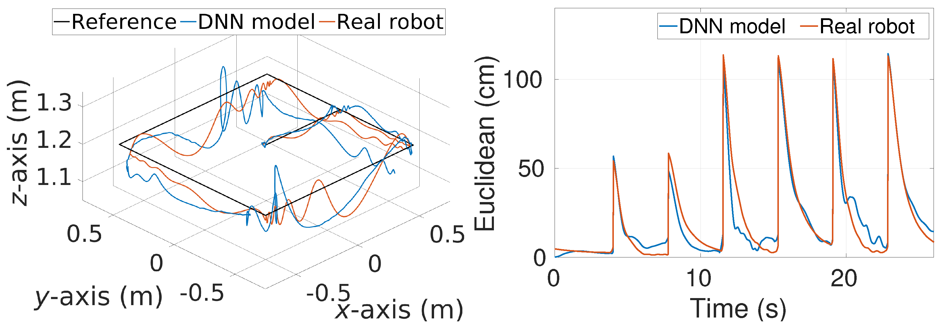
6.2. Real Flight Tuning

The best weight set from real flight tuning is:

$$\begin{array}{c}\hfill \begin{array}{cc}\hfill W_{\mathtt{x}}^{*}& =\mathrm{diag}(17,11,14,1.5,1.8,1.9),\hfill \\ \hfill W_{\mathtt{u}}^{*}& =\mathrm{diag}(20,15,68,0.064).\hfill \end{array}\end{array}$$

(14)

For hovering, this weight set results in a precise tracking with mean Euclidean error values of 3–4 cm over both the DNN model and real robot, as evident in Figure 6. In terms of the sequential-setpoint tracking, it again yields precise tracking performance with the mean Euclidean error values of around 18 cm (Figure 6) which are slightly less compared to the ones in the former subsection. This exhibits the tracking improvement by fine-tuning in real flights.

We repeated the above experiments with the ten best weight sets from real flight tuning and the complete right side of Figure 5. While the average and maximum error values for hovering with the DNN model were $2.63$ and $2.85$ cm, they increased slightly over the real robot to $4.54$ and $6.12$ cm. As for the sequential setpoints, the average and maximum error values changed from $19.43$ and $21.16$ cm over the DNN model to $18.49$ and $21.7$ cm over the real robot.

An important comment that need to be made about Figure 5 is that the respective average and maximum mean Euclidean error values obtained over the real robot for hovering reduce from $5.11$ and $7.94$ cm to $4.54$ and $6.12$ cm after the real flight tuning, which implies $11.15\%$ and $22.92\%$ improvements in these values. For the sequential-setpoint tracking case, these numbers reduce from $22.21$ and $28.27$ cm to $18.49$ and $21.7$ cm, which suggests a performance improvement by $16.75\%$ and $23.24\%$ in terms of average and maximum mean Euclidean errors. These small improvements both show the high fidelity of the DNN model and reveal the possible benefits of fine-tuning in real flights.

Remark 5.

As already known, the tracking performance of NMPC for any trajectory is critically linked to a specific weight set. That is, if a weight set performs best for one trajectory, it is not guaranteed to do the same for other time-based trajectories. This limitation also exists with the weight set obtained by the auto-tuning algorithm. Nevertheless, the users can accordingly select/add the flight configurations keeping in mind the trajectories of interest.

6.3. User-Based Tuning Study

To further analyze the proposed auto-tuning method’s efficacy, we conducted a user-based tuning study for comparison. Ten users with different quadrotor backgrounds were given the task of tuning NMPC over a Gazebo model of our quadrotor for two hours. We recorded two weight sets from each user: one after the first hour and one after the second hour of tuning. We then performed trajectory tracking over the DNN model to evaluate the performance of these weight sets. One may note that evaluation of these weights over the real robot was avoided due to safety reasons.

Remark 6.

The motivation to adopt the Gazebo simulation platform is its rendering capability by which the robot’s response can be visually observed. In this way, the overall tuning process mimics the manual tuning of the robot in real flights.

The resulting mean Euclidean errors are listed in

Table 6. Mean Euclidean error and the corresponding oscillatory response for the weight sets obtained by user-based tuning. Accordingly, the weight sets whose results are marked with bold font are regarded as real flight-worthy.

	First Hour				Second Hour
	Hover		Sequential-Setpoints		Hover		Sequential-Setpoints
	Mean Euc. Error (cm)	Number of Oscillations	Mean Euc. Error (cm)	Number of Oscillations	Mean Euc. Error (cm)	Number of Oscillations	Mean Euc. Error (cm)	Number of Oscillations
User 1	$12.70$	31	$1.21\times {10}^5$	176	$4.83$	1	$1.10\times {10}^4$	204
User 2	$30.64$	20	$3.09\times {10}^4$	220	$34.51$	20	$89.47$	34
User 3	$15.10$	34	$7.21\times {10}^4$	138	$14.42$	29	$1.03\times {10}^5$	232
User 4	$10.74$	20	$25.74$	50	$10.09$	18	$38.13$	47
User 5	$13.29$	36	$7.82\times {10}^4$	146	$\mathbf{6}.\mathbf{24}$	$\mathbf{0}$	$\mathbf{23}.\mathbf{41}$	$\mathbf{17}$
User 6	$3.96$	2	$24.87$	37	$12.46$	19	$33.78$	45
User 7	$\mathbf{5}.\mathbf{28}$	$\mathbf{0}$	$\mathbf{35}.\mathbf{11}$	$\mathbf{5}$	$9.70$	6	$31.88$	31
User 8	$\mathbf{3}.\mathbf{41}$	$\mathbf{3}$	$\mathbf{22}.\mathbf{01}$	$\mathbf{21}$	$2.69$	0	$23.62$	44
User 9	$8.50$	16	$4.36\times {10}^6$	250	$4.20$	1	$36.55$	29
User 10	$3.02$	0	$38.26$	32	$8.23$	10	$26.78$	35

along with the observed number of oscillations, depicting the oscillatory behavior of a particular weight set. It is to be noted that oscillation is characterized as an abrupt change of more than 3 cm in the Euclidean error response. As can be seen, most users resulted in high Euclidean errors with moderate to high oscillations, implying an eventual crash of the robot, whereas three users obtained the real flight-worthy weight sets (marked with bold-font), which accounts for only 15% success. We would like to emphasize that most users could obtain some meaningful weight sets in a limited time as they could try abrupt values over the simulation model which otherwise might not be possible over the real robot. Essentially, the proper tuning procedure in a general case takes around 3–4 h (or even more), as noticed in our informal observations. Another point to take note in Table 6 is that for almost half of the users, the tracking performance decreased from the first to the second hour of tuning. This is counterintuitive as one expects to perform better after gaining some experience with the system. Nevertheless, utilizing the relation in (12), the proposed algorithm always looks for the weight sets which could perform better by satisfying stricter criteria.

For a quantitative comparison, we deployed the best weight set from user-based tuning (User 8 after the first hour) with the best one obtained from simulation-based tuning (given in (13)) for hover and sequential-setpoint tracking of the DNN model. The comparison plots are given in Figure 7. While the corresponding mean Euclidean error values for the user-based weight set are $3.41$ cm and $22.01$ cm, the proposed algorithm outperforms it by resulting in error values of $2.85$ cm and $21.16$ cm, respectively. In addition, in terms of the number of oscillations, the user-based weight set has values of 3 and 21 for hover and sequential setpoints, respectively, whereas the auto-tuned weight set has values of 0 and 9, respectively. These values are significantly less when compared to the user-based weight set, thereby implying a safer weight set. All these results signify that the proposed method can realize better weight sets in a limited time (less than an hour) that an average user cannot obtain even after two hours.

7. Conclusions

In this work, we have aimed to tackle one of the arduous yet unavoidable tasks for the real-time implementation of MPC on robots. We have presented a novel, active exploration-based tuning framework for obtaining MPC weight sets. To avoid the weight set trials on the real robot for the sake of safety, we have incorporated a DNN model. Thanks to its high fidelity, it has facilitated the direct utilization of the obtained weight sets on the real robot. We have also demonstrated fine-tuning over the real robot. Extensive statistical analysis, real flight trajectory tracking results, and a comparative user study validate that this work could help researchers with the real-time implementation of their MPCs by saving a considerable amount of tuning time without compromising the safety of the robot.

As future work, we intend to update the DNN model such that it incorporates effects such as sensor noise and modeling uncertainties. This will result in a stochastic model of the overall system, thereby further justifying the usage of the active-exploration paradigm. Furthermore, to enhance the generalization of the auto-tuning framework, we aim to eliminate heuristics, such as including reasonable bounds on search space, which require some domain knowledge.

References

1. Ortiz, A.; Garcia-Nieto, S.; Simarro, R. Comparative Study of Optimal Multivariable LQR and MPC Controllers for Unmanned Combat Air Systems in Trajectory Tracking. Electronics 2021, 10, 331. [Google Scholar] [CrossRef]
2. Ahn, T.; Lee, Y.; Park, K. Design of Integrated Autonomous Driving Control System That Incorporates Chassis Controllers for Improving Path Tracking Performance and Vehicle Stability. Electronics 2021, 10, 144. [Google Scholar] [CrossRef]
3. Mehndiratta, M.; Kayacan, E. Gaussian Process-based Learning Control of Aerial Robots for Precise Visualization of Geological Outcrops. In Proceedings of the 2020 European Control Conference (ECC), St. Petersburg, Russia, 12–15 May 2020; pp. 10–16. [Google Scholar]
4. Imanberdiyev, N.; Kayacan, E. Redundancy Resolution based Trajectory Generation for Dual-Arm Aerial Manipulators via Online Model Predictive Control. In Proceedings of the IECON 2020 The 46th Annual Conference of the IEEE Industrial Electronics Society, Singapore, 18–21 October 2020; pp. 674–681. [Google Scholar] [CrossRef]
5. Mehndiratta, M.; Kayacan, E.; Patel, S.; Kayacan, E.; Chowdhary, G. Learning-based Fast Nonlinear Model Predictive Control for Custom-made 3D Printed Ground and Aerial Robots. Control Eng. 2019. [Google Scholar] [CrossRef]
6. Bai, G.; Meng, Y.; Liu, L.; Luo, W.; Gu, Q.; Liu, L. Review and Comparison of Path Tracking Based on Model Predictive Control. Electronics 2019, 8, 1077. [Google Scholar] [CrossRef] [Green Version]
7. Mehndiratta, M.; Kayacan, E. A constrained instantaneous learning approach for aerial package delivery robots: Onboard implementation and experimental results. Auton. Robots 2019, 43, 2209–2228. [Google Scholar] [CrossRef]
8. Baca, T.; Hert, D.; Loianno, G.; Saska, M.; Kumar, V. Model Predictive Trajectory Tracking and Collision Avoidance for Reliable Outdoor Deployment of Unmanned Aerial Vehicles. In Proceedings of the 2018 IEEE/RSJ International Conference on Intelligent Robots and Systems (IROS), Madrid, Spain, 1–5 October 2018; pp. 6753–6760. [Google Scholar] [CrossRef]
9. Mehndiratta, M.; Kayacan, E. Reconfigurable Fault-tolerant NMPC for Y6 Coaxial Tricopter with Complete Loss of One Rotor. In Proceedings of the 2018 IEEE Conference on Control Technology and Applications (CCTA), Copenhagen, Denmark, 21–24 August 2018; pp. 774–780. [Google Scholar] [CrossRef]
10. Mehndiratta, M.; Kayacan, E. Online Learning-based Receding Horizon Control of Tilt-rotor Tricopter: A Cascade Implementation. In Proceedings of the 2018 American Control Conference (ACC), Milwaukee, WI, USA, 27–29 June 2018; pp. 1–6. [Google Scholar]
11. Mehndiratta, M.; Kayacan, E. Receding horizon control of a 3 DOF helicopter using online estimation of aerodynamic parameters. Proc. Inst. Mech. Eng. Part J. Aerosp. Eng. 2017. [Google Scholar] [CrossRef]
12. Eren, U.; Prach, A.; Koçer, B.B.; Raković, S.V.; Kayacan, E.; Açikmeşe, B. Model Predictive Control in Aerospace Systems: Current State and Opportunities. J. Guid. Control Dyn. 2017, 40, 1541–1566. [Google Scholar] [CrossRef]
13. Lee, W.Y.J.; Mehndiratta, M.; Kayacan, E. Fly without borders with additive manufacturing: A microscale tilt-rotor tricopter design. In Proceedings of the 3rd International Conference on Progress in Additive Manufacturing (Pro-AM 2018), Singapore, 14–17 May 2018; pp. 256–261. [Google Scholar] [CrossRef]
14. Kayacan, E.; Kayacan, E.; Ramon, H.; Saeys, W. Learning in Centralized Nonlinear Model Predictive Control: Application to an Autonomous Tractor-Trailer System. IEEE Trans. Control Syst. Technol. 2015, 23, 197–205. [Google Scholar] [CrossRef]
15. Lee, J.; Yu, Z. Tuning of model predictive controllers for robust performance. Comput. Chem. Eng. 1994, 18, 15–37. [Google Scholar] [CrossRef]
16. Shridhar, R.; Cooper, D.J. A Tuning Strategy for Unconstrained Multivariable Model Predictive Control. Ind. Eng. Chem. Res. 1998, 37, 4003–4016. [Google Scholar] [CrossRef]
17. Di Cairano, S.; Bemporad, A. Model Predictive Control Tuning by Controller Matching. IEEE Trans. Autom. Control 2010, 55, 185–190. [Google Scholar] [CrossRef]
18. Ali, E.; Zafiriou, E. Optimization-based tuning of nonlinear model predictive control with state estimation. J. Process Control 1993, 3, 97–107. [Google Scholar] [CrossRef] [Green Version]
19. Al-Ghazzawi, A.; Ali, E.; Nouh, A.; Zafiriou, E. On-line tuning strategy for model predictive controllers. J. Process Control 2001, 11, 265–284. [Google Scholar] [CrossRef]
20. Ali, E. Heuristic on-line tuning for nonlinear model predictive controllers using fuzzy logic. J. Process Control 2003, 13, 383–396. [Google Scholar] [CrossRef]
21. Shipman, W.J.; Coetzee, L.C. Reinforcement Learning and Deep Neural Networks for PI Controller Tuning. IFAC-PapersOnLine 2019, 52, 111–116. [Google Scholar] [CrossRef]
22. Kofinas, P.; Dounis, A.I. Fuzzy Q-Learning Agent for Online Tuning of PID Controller for DC Motor Speed Control. Algorithms 2018, 11, 148. [Google Scholar] [CrossRef] [Green Version]
23. Junell, J.; Mannucci, T.; Zhou, Y.; Van Kampen, E.J. Self-tuning gains of a quadrotor using a simple model for policy gradient reinforcement learning. In Proceedings of the AIAA Guidance, Navigation, and Control Conference, San Diego, CA, USA, 4–8 January 2016; p. 1387. [Google Scholar]
24. Howell, M.; Best, M. On-line PID tuning for engine idle-speed control using continuous action reinforcement learning automata. Control Eng. Pract. 2000, 8, 147–154. [Google Scholar] [CrossRef] [Green Version]
25. Mehndiratta, M.; Camci, E.; Kayacan, E. Automated Tuning of Nonlinear Model Predictive Controller by Reinforcement Learning. In Proceedings of the 2018 IEEE/RSJ International Conference on Intelligent Robots and Systems (IROS), Madrid, Spain, 1–5 October 2018. [Google Scholar]
26. Bouabdallah, S. Design and Control of Quadrotors with Application to Autonomous Flying. Ph.D. Thesis, EPFL, Swiss Federal Institute of Technology Lausanne, Lausanne, Switzerland, 2007. [Google Scholar]
27. Kraus, T.; Ferreau, H.; Kayacan, E.; Ramon, H.; Baerdemaeker, J.D.; Diehl, M.; Saeys, W. Moving horizon estimation and nonlinear model predictive control for autonomous agricultural vehicles. Comput. Electron. Agric. 2013, 98, 25–33. [Google Scholar] [CrossRef]
28. Du, X.; Htet, K.K.K.; Tan, K.K. Development of a Genetic-Algorithm-Based Nonlinear Model Predictive Control Scheme on Velocity and Steering of Autonomous Vehicles. IEEE Trans. Ind. Electron. 2016, 63, 6970–6977. [Google Scholar] [CrossRef]
29. Diehl, M.; Bock, H.; Schlöder, J.P.; Findeisen, R.; Nagy, Z.; Allgöwer, F. Real-time optimization and nonlinear model predictive control of processes governed by differential-algebraic equations. J. Process Control 2002, 12, 577–585. [Google Scholar] [CrossRef]
30. Kingma, D.P.; Ba, J. Adam: A method for stochastic optimization. arXiv 2014, arXiv:1412.6980. [Google Scholar]
31. Camci, E.; Campolo, D.; Kayacan, E. Deep Reinforcement Learning for Motion Planning of Quadrotors Using Raw Depth Images. In Proceedings of the 2020 International Joint Conference on Neural Networks (IJCNN), Glasgow, UK, 19–24 July 2020; pp. 1–7. [Google Scholar]
32. Sutton, R.S.; Barto, A.G. Reinforcement Learning: An Introduction; MIT Press: Cambridge, UK, 1998; Volume 1. [Google Scholar]
Figure 1. Custom-made quadrotor of interest. Notation: F i and τ i are the force and torque generated by i th rotor with Ω i angular velocity; τ x , τ y , τ z are the external moments about x-, y-, z-axes, respectively.
Electronics 10 02187 g001
Figure 2. Proposed (N)MPC weight tuning framework. Throughout the tuning process, each trial starts with the Trial Configuration module. Weight set selection and Stable flight mode submodules give necessary instructions to (N)MPC. Taking these as inputs, (N)MPC controls the quadrotor model while its performance is being observed simultaneously. Once a flight is completed, the performance of the (N)MPC with the utilized weight set is graded based on the five criteria. Subsequently, the trial is finalized by updating the weight set cluster. Thereafter, a new trial begins with the selection of a new weight set within the Trial Configuration module, and thus closes the loop.
Electronics 10 02187 g002
Figure 3. Hovering performance of the weight set obtained from simulation tuning. (Left): 3D view of the stationary reference and tracked trajectories. (Right): resulting Euclidean error over the DNN model and the real robot.
Electronics 10 02187 g003
Figure 4. Sequential-setpoints tracking performance of the weight set obtained from simulation tuning. (Left): 3D view of the sequential-setpoints and tracked trajectories. (Right): resulting Euclidean error over the DNN model and the real robot.
Electronics 10 02187 g004
Figure 5. Boxplot of mean Euclidean error obtained by the weight sets having top ten grade values in the lookup tables from simulation (Left) and real flight (Right) tuning.
Electronics 10 02187 g005
Figure 6. Euclidean errors for hover (Left) and for sequential-setpoints (Right) by the weight set from real flight tuning.
Electronics 10 02187 g006
Figure 7. Euclidean errors for hover (Left) and for sequential setpoints (Right) by the best weight sets from simulation and user-based tuning.
Electronics 10 02187 g007