Analysis of Singular Configuration of Robotic Manipulators

Abstract

Robotic manipulators inevitably encounter singular configurations in the process of movement, which seriously affects their performance. Therefore, the identification of singular configurations is extremely important. However, serial manipulators that do not meet the Pieper criterion cannot obtain singular configurations through analytical methods. A joint angle parameterization method, used to obtain singular configurations, is here creatively proposed. First, an analytical method based on the Jacobian determinant and the proposed method were utilized to obtain their respective singular configurations of the Stanford manipulator. The singular configurations obtained through the two methods were consistent, which suggests that the proposed method can obtain singular configurations correctly. Then, the proposed method was applied to a seven-degree-of-freedom (7-DOF) serial manipulator and a planar 5R parallel manipulator. Finally, the correctness of the singular configurations of the 7-DOF serial manipulator was verified through the shape of the end-effector velocity ellipsoid, the value of the determinant, the value of the condition number, and the value of the manipulability measure. The correctness of singular configurations of the planar 5R parallel manipulator was verified through the value of the determinant, the value of the condition number, and the value of the manipulability measure.

1. Introduction

It is well-known that the kinematics of robotic manipulators can be expressed on the velocity level, and the relationship between the joint velocities and end-effector (EE) velocities is described by a Jacobian matrix. Robotic manipulators that do not meet the Pieper criterion [1] only obtain a numerical solution to the inverse kinematics, and the Jacobian iteration algorithm is a commonly algorithm for numerical solution. However, when robotic manipulators approach a singular configuration, the Jacobian matrix becomes numerically unrealizable, and this is experienced in the form of high joint velocities, which are not conducive to motion control. Therefore, the identification of singular configurations is a key issue to avoid singularity. Singularity in robotic manipulators includes boundary singularity and internal singularity [2]. Boundary singularity appears at the working space boundary, and internal singularity is caused by the coincidence of two or more joint axes. Robotic manipulators are divided into serial manipulators and parallel manipulators from the perspective of mechanism [3]. Müller [4] roughly classified the singularities of serial manipulators and parallel manipulators based on active and passive joints and proposed an algorithm to determine the singularities of the mechanism. Most researchers have performed singularity analysis on serial manipulators or parallel manipulators. The following concerns parallel manipulators. Li [5] introduced a cell-division method for singularity analysis, which could be used to multi-loop mechanisms. The key principle was replacing the singularity analysis of the original multi-loop mechanism with an equivalent and simpler parallel mechanism. Han [6] proposed a simple and effective method to determine the singularity of planar linkages. Chen [7] analyzed the singularities of the 3-UPU (U stands for the universal joint and the prismatic pair P is actuated) parallel mechanism. Nayak [8] carried out a singularity analysis for a serial-parallel robot. Ma [9] proposed a singularity analysis method for a 3/6-SPS Gough-Stewart parallel manipulator based on geometric algebra, in which S represents the spherical joint and P represents the prismatic pair. Wu [10] obtained singular configurations of three configurations of parallel manipulators using an analytical method. However, this method does not necessarily guarantee that it can be applied to other configurations of parallel manipulators. Ben-Horin [11] solved the singularities of a general class of Gough-Stewart platforms through Grassmann–Cayley algebra. Conconi [12] analyzed the causes of the singular events of parallel kinematic chains and identified singular configurations. Pagis [13] transformed near-singularities into a simplified dynamic model to allow parallel manipulators to cross the type 2 singularity with the best trajectory.

We now look at serial manipulators that meet the Pieper criterion. For these manipulators, three revolute axes intersect at a point, and singular configurations can be obtained by solving the determinant so that it is zero. Li [14] analyzed singular configurations of a six-degree-of-freedom (6-DOF) modular robotic manipulator. Yu [15] divided singularity into forearm singularity and wrist singularity and took measures to avoid them. Carmichael [16] only described the situation in which singular configurations occur when the singular value is zero, and this is far away from singular configurations through a virtual force. Furthermore, singular configurations of the manipulator were not obtained. Kang [17] carried out singularity analysis of a 6-DOF anthropomorphic manipulator and proposed two solutions to avoid boundary singularity and internal singularity. Xu [18] determined singular configurations based on the Jacobian matrix of a non-spherical wrist manipulator. However, the method is only suitable for a manipulator with a specific configuration and has low applicability. Hijazi [19] analyzed the singularities of a planar robot manipulator in redundant and non-redundant cases. Although singularity surfaces were obtained, singular configurations were avoided through trajectory planning. Müller [20] carried out high-order analysis of motion singularity for serial manipulators. However, the derivation and calculation process were complex, which is not suitable for singularity analysis of redundant manipulators. Oetomo [21] introduced singular configurations of the PUMA 560 and analyzed the associated singular directions and the handling algorithm.

However, there are also serial manipulators that do not meet the Pieper criterion. The determinant of the Jacobian matrix is especially complex and cannot be simplified effectively, so it is difficult to obtain singular configurations through analytical methods. Rebouças Filho [22] used a genetic algorithm to identify and solve singular problems along the trajectory of a robotic manipulator. However, the method identified singular regions rather than specific singular configurations. In [23], the singularity of a 6-DOF painting robot with a non-spherical wrist was decomposed into position singularity and attitude singularity by introducing a virtual wrist center. Due to the virtual wrist center, the D-H parameters d_i of the 7R 6-DOF manipulator changed, so an error was introduced to the position of the EE. Dimeas [24] determined the position singularity through the distribution curve of the manipulability, the minimum singular value, and the local condition index. However, this method ignored attitude singularity.

Serial manipulators that meet the Pieper criterion can obtain singular configurations through an analytical method. However, for serial manipulators that do not meet the Pieper criterion, most studies on the subject focus on singularities of special manipulators or on avoiding singular regions. Singular configurations when a singular value is zero are less commonly studied. Therefore, a joint angle parameterization method to obtain singular configurations is here proposed. The remainder of this paper is organized as follows: The kinematics of robotic manipulators is briefly reviewed in Section 2. Singular configurations of a Stanford manipulator are obtained through an analytical method in Section 3.1. In Section 3.2, a joint angle parameterization method is proposed to identify singular configurations and applied to the Stanford manipulator, a 7-DOF serial manipulator, and a planar 5R parallel manipulator. In Section 4, the correctness of the singular configurations of the 7-DOF serial manipulator obtained by the proposed algorithm is verified through the shape of the EE velocity ellipsoid, the value of the determinant, the value of the condition number, and the value of the manipulability measure. The correctness of the singular configurations of the planar 5R parallel manipulator obtained by the proposed algorithm is verified through the value of the determinant, the value of the condition number, and the value of the manipulability measure. Finally, the conclusions and direction for future work are presented in Section 5.

2. Related Work

The forward kinematics on the velocity level can be described as follows:

$$\dot{\mathit{x}} =\mathit{J} \dot{\mathit{q}}$$

(1)

where $\dot{\mathit{x}} \in {\mathit{R}}^{\mathit{m}}$ is the velocity vector of the EE, $\dot{\mathit{q}} \in {\mathit{R}}^{\mathrm{n}}$ represents the velocity vector of the joint, and $\mathit{J}\in {\mathit{R}}^{\mathit{m}\times \mathrm{n}}$ is a Jacobian matrix.

The inverse kinematics on the velocity level for non-redundant manipulators is:

$${ \dot{\mathit{q}} =\mathit{J}}^{-1} \dot{\mathit{x}}$$

(2)

and for redundant manipulators it is

$${ \dot{\mathit{q}} =\mathit{J}}^{+}{ \dot{\mathit{x}} =\mathit{J}}^{\mathrm{T}}{\left({\mathit{JJ}}^{\mathrm{T}}\right)}^{-1} \dot{\mathit{x}}$$

(3)

Equations (2) and (3) hold when ${\mathit{J}}^{-1}$ or ${\mathit{J}}^{+}$ exists, and Equation (3) provides a least-norm solution.

Singularity occurs when the determinant of the Jacobian matrix is zero:

$$\det \left(\mathit{J}\right)=0$$

(4)

$$\det \left({\mathit{JJ}}^{\mathrm{T}}\right)=0$$

(5)

Singular value decomposition [25,26] can explain the effect of singularity more clearly. With $\mathit{J}$ ranked $\mathit{r}$, $\mathit{J}$ is described as $\mathit{J}=\mathbf{U}\mathsf{\Sigma }{\mathbf{V}}^{\mathrm{T}}={\displaystyle \sum _{i=1}^m{\sigma }_i{u}_i{v}_i^{\mathrm{T}}}$, where $\mathbf{U}$ is the $\mathit{m}\times \mathit{m}$ matrix of the output singular vectors ${\mathrm{u}}_{\mathit{i}}$ and $\mathbf{V}$ is the $\mathit{n}\times \mathit{n}$ matrix of the input singular vectors ${\mathrm{v}}_{\mathit{i}}$.

$$\begin{array}{c}\mathsf{\Sigma }\end{array}=\left[\begin{array}{cc}\mathrm{diag}{\left({\sigma }_1,{\sigma }_2,\cdot \cdot \cdot ,{\sigma }_r\right)}_{r\times r}& 0_{r\times \left(n-r\right)}\\ 0_{\left(m-r\right)\times r}& 0_{\left(m-r\right)\times \left(n-r\right)}\end{array}\right]$$

(6)

${\sigma }_1\ge {\sigma }_2\ge \cdot \cdot \cdot \ge {\sigma }_{\mathrm{r}}>0$, ${\sigma }_{\mathrm{r}+1}=\cdot \cdot \cdot ={\sigma }_{\mathit{m}}=0$. Hence, ${\mathit{J}}^{-1}$ and ${\mathit{J}}^{+}$ can be represented as follows:

$${\mathit{J}}^{-1}=\mathbf{V}{\mathsf{\Sigma }}^{-1}{\mathbf{U}}^{\mathrm{T}}={\displaystyle \sum _{\mathit{i}=1}^{\mathit{m}}\frac{1}{{\sigma }_{\mathit{i}}}{\mathit{v}}_{\mathit{i}}{\mathit{u}}_{\mathit{i}}^{\mathrm{T}}}$$

(7)

$${\mathit{J}}^{+}{=\mathit{J}}^{\mathrm{T}} \overline{\mathbf{V}} {\left( \overline{\mathsf{\Sigma }} \right)}^{-1}{ \overline{\mathbf{U}} }^{\mathrm{T}}{=\mathit{J}}^{\mathrm{T}}{\displaystyle \sum _{\mathit{i}=1}^{\mathit{m}}\frac{1}{{\overline{\sigma }}_{\mathit{i}}}{ \overline{\mathit{v}} }_{\mathit{i}}{ \overline{\mathit{u}} }_{\mathit{i}}^{\mathrm{T}}}$$

(8)

Thus, Equations (2) and (3) can be described as:

$$\dot{\mathit{q}} ={\displaystyle \sum _{i=1}^m\frac{1}{{\sigma }_i}{v}_i{u}_i^{\mathrm{T}}} \dot{\mathit{x}}$$

(9)

$${ \dot{\mathit{q}} =\mathit{J}}^{\mathrm{T}}{\displaystyle \sum _{i=1}^{\mathit{m}}\frac{1}{{\overline{\sigma }}_i}{\overline{v}}_i{\overline{u}}_i^{\mathrm{T}}} \dot{\mathit{x}}$$

(10)

When robotic manipulators approach a singular configuration, the Jacobian (pseudo-) inverse values become numerically unstable and unrealizable. Therefore, the identification of singular configurations of robotic manipulators is the key to solving the singularity problem.

3. A Novel Singularity Identification Method

First, singular configurations of a Stanford manipulator are obtained through an analytical method based on the Jacobian determinant. Then, a singular configuration identification method based on joint angle parameterization is proposed and applied to the Stanford manipulator. Singular configurations obtained through the proposed method are compared with the results through the analytical method, which verifies the correctness of the proposed method. Furthermore, the proposed method is applied to a 7-DOF serial manipulator and a planar 5R parallel manipulator.

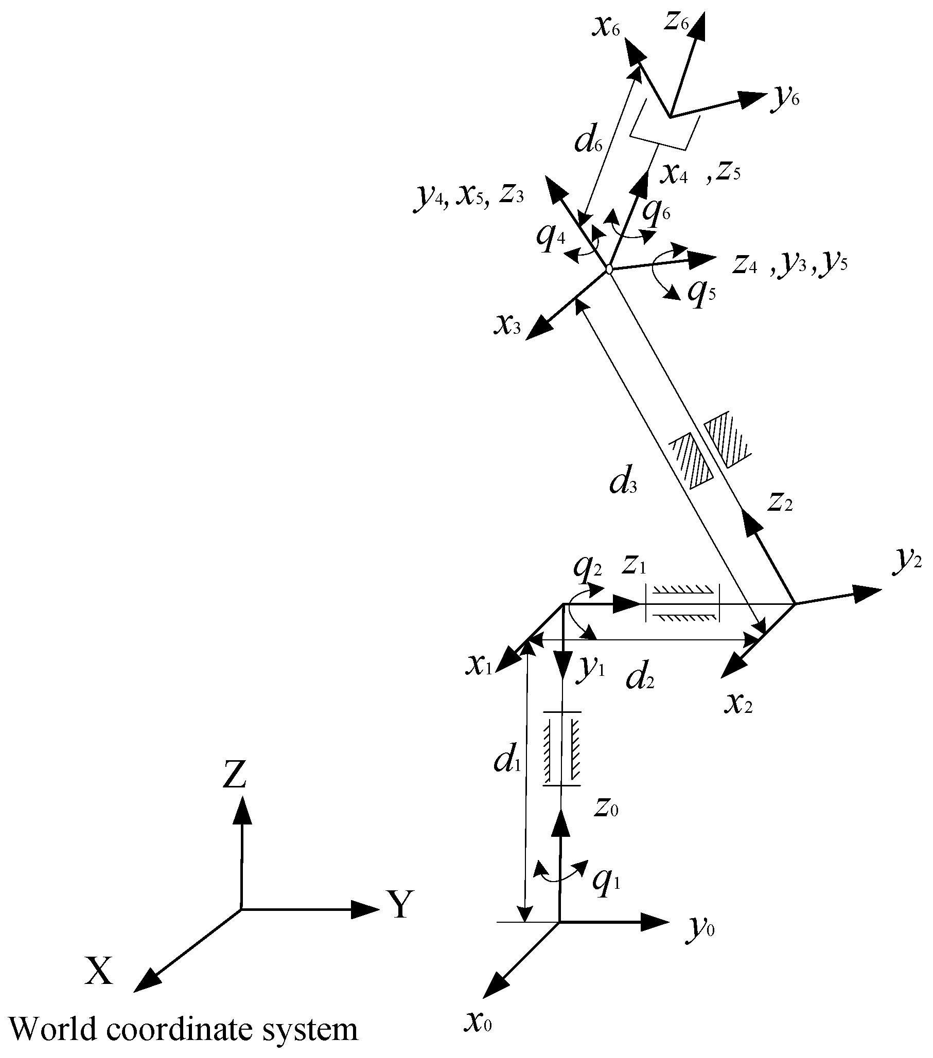
3.1. Determining Singular Configurations of a Stanford Manipulator through an Analytical Method

The Stanford manipulator [27] is a classic industrial manipulator that meets the Pieper criterion. Singular configurations of this manipulator can be obtained through an analytical method. The coordinate system and standard DH parameters are shown in Figure 1 and

Table 1. Standard DH parameters of the Stanford manipulator.

i	${\mathit{\alpha }}_{\mathbf{i}} \left(\mathbf{rad}\right)$	${\mathit{a}}_{\mathbf{i}} \left(\mathbf{m}\right)$	${\mathit{d}}_{\mathbf{i}} \left(\mathbf{m}\right)$	${\mathit{q}}_{\mathbf{i}} \left(\mathbf{rad}\right)$	$[{\mathit{q}}_{\mathbf{imin}},{\mathit{q}}_{\mathbf{imax}}]$
1	$-\mathsf{\pi }/2$	0	0.08	$q_1$	$[-\mathsf{\pi },\mathsf{\pi }]\left(\mathrm{rad}\right)$
2	$\mathsf{\pi }/2$	0	0.06	$q_2$	$[-\mathsf{\pi },\mathsf{\pi }]\left(\mathrm{rad}\right)$
3	0	0	${\mathit{d}}_3$	0	$[-0.5,0.5]\left(\mathrm{m}\right)$
4	$-\mathsf{\pi }/2$	0	0	$q_4$	$[-\mathsf{\pi },\mathsf{\pi }]\left(\mathrm{rad}\right)$
5	$\mathsf{\pi }/2$	0	0	$q_5$	$[-\mathsf{\pi },\mathsf{\pi }]\left(\mathrm{rad}\right)$
6	0	0	0.08	$q_6$	$[-\mathsf{\pi },\mathsf{\pi }]\left(\mathrm{rad}\right)$

.

The $\mathit{J}$ obtained by the differential transformation method is

$$\mathit{J}=\left[\begin{array}{cc}{\mathit{J}}_{11}& 0\\ {\mathit{J}}_{21}& {\mathit{J}}_{22}\end{array}\right]$$

(11)

where ${\mathit{J}}_{11}$, ${\mathit{J}}_{21}$, and ${\mathit{J}}_{22}$ are reflected in Appendix A. It is easy to calculate $\left|{\mathit{J}}_{11}\right|=- {\mathit{d}}_3^2\sin q_2$, $\left|{\mathit{J}}_{22}\right|=- \sin q_5$. Using Equation (4), it is not difficult to see that singular configurations occur in $q_2= 0$, $\pm \mathsf{\pi }$; ${\mathit{d}}_3=0$; and $q_5=0$, $\pm \mathsf{\pi }$.

3.2. A Singular Configuration Identification Method Based on Joint Angle Parameterization

This section and Section 4 were developed using the MATLAB R2015a tool, and an Intel Core™ i5-2450M CPU @ 2.50 GHz and 2 GB RAM control platform was used to run it.

In view of the fact that singular configurations of robotic manipulators appear when a joint angle is $0$, $\pm \mathsf{\pi }/2$, $\pm \mathsf{\pi }$, or more, the joint angles are here considered to be $0$, $\pm \mathsf{\pi }/2$, $\pm \mathsf{\pi }$. A joint angle parameterization method to determine singular configurations based on these special angles is proposed. The method steps are as follows:

(1)

A group of joint positions to be applied in the subsequent steps are arbitrarily chosen to satisfy $\det \left(\mathit{J}\right)\ne 0$;

(2)

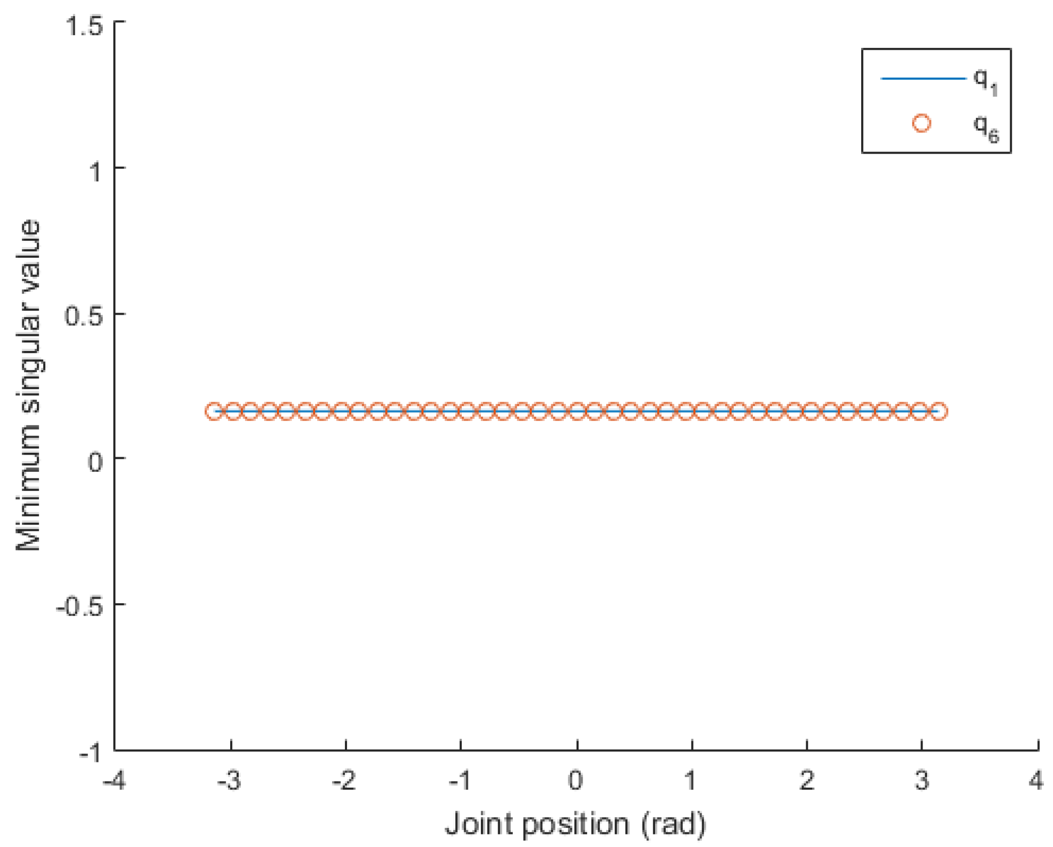
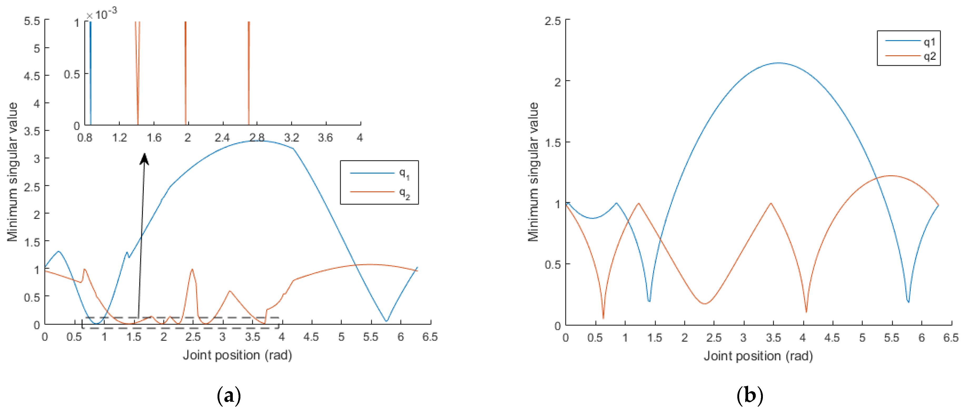
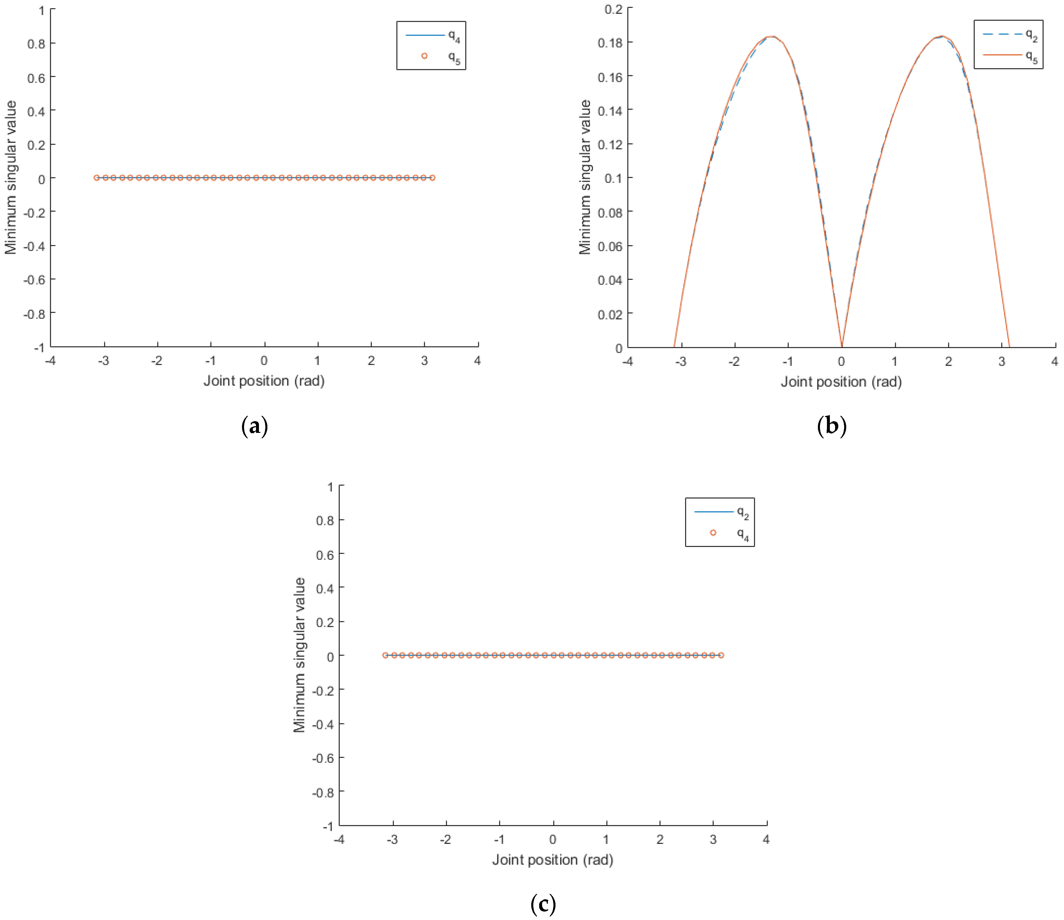
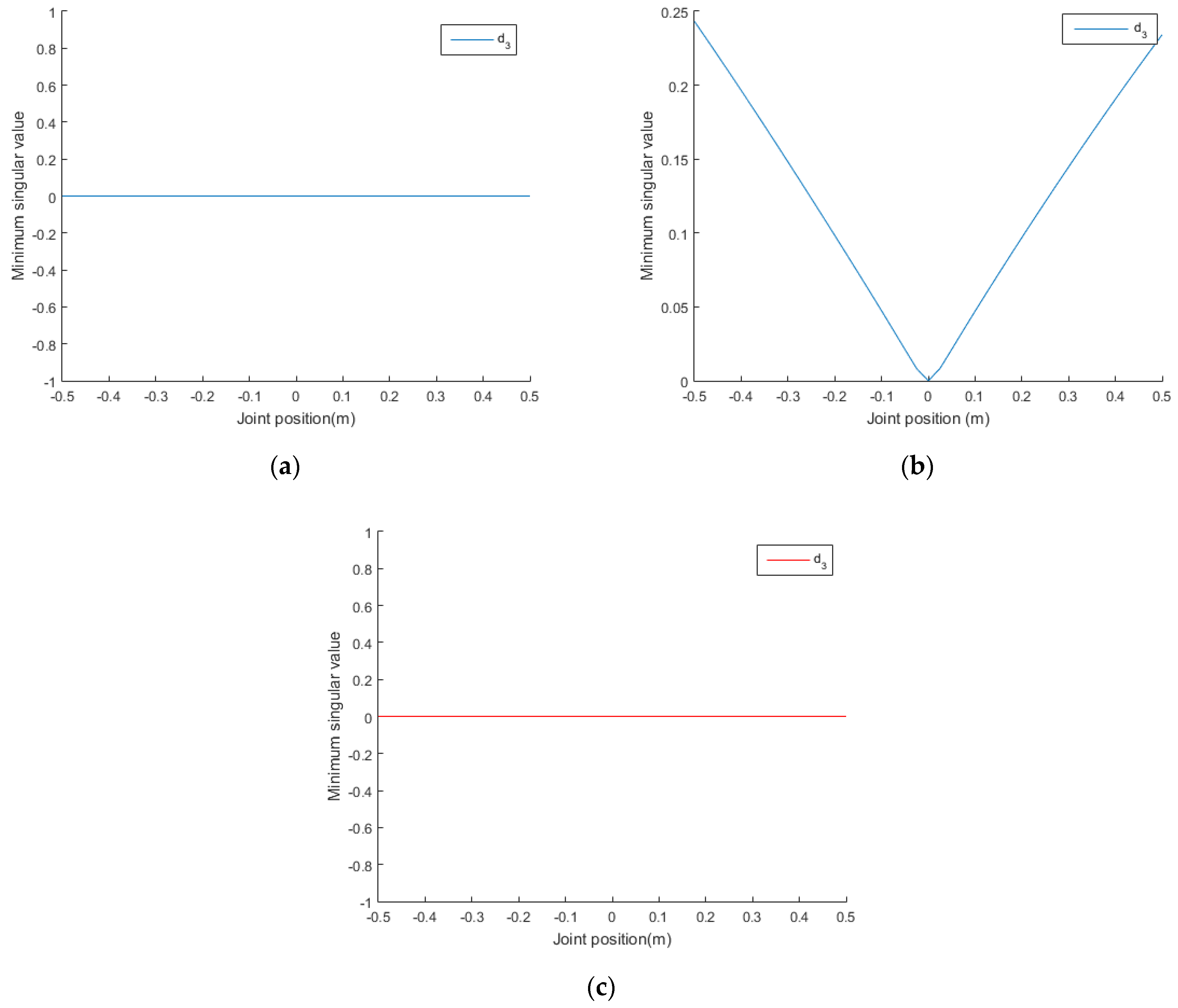
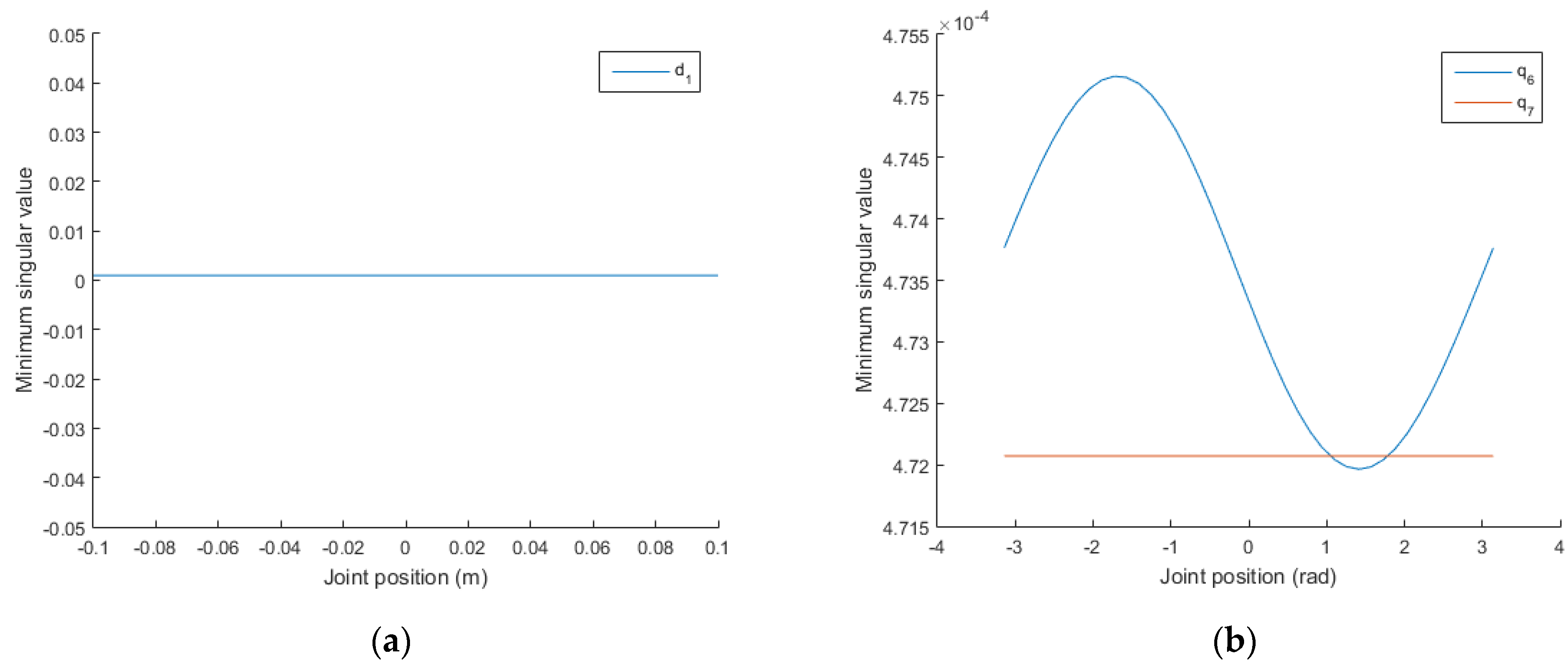
First, all joint positions are set to $0$, $\pm \mathsf{\pi }/2$, $\pm \mathsf{\pi }$, respectively, and substituted into Equation (4) or Equation (5). If the determinant is not zero, it means that this group of joint positions will not produce singularity, and these joint positions can be ignored in the subsequent steps. Then, on the basis of the set of joint positions in step 1, a joint position is selected and set to $0$, $\pm \mathsf{\pi }/2$, $\pm \mathsf{\pi }$. From the remaining joints, a joint is selected and varied within its range, and the other joint positions remain unchanged. Finally, the distribution of the minimum singular value with the change in a joint position is obtained. For example, for a 6-DOF manipulator, $q_1=0$, $q_3=q_4=q_5=q_6=\mathsf{\pi }/3$, and $q_2\in [-\mathsf{\pi },\mathsf{\pi }]$ are set. Finally, the distribution of the minimum singular value with the change in $q_2$ is obtained. In the same way, the distributions of the minimum singular values with the changes of $q_3$, $q_4$, $q_5$, and $q_6$ are also obtained;

(3)

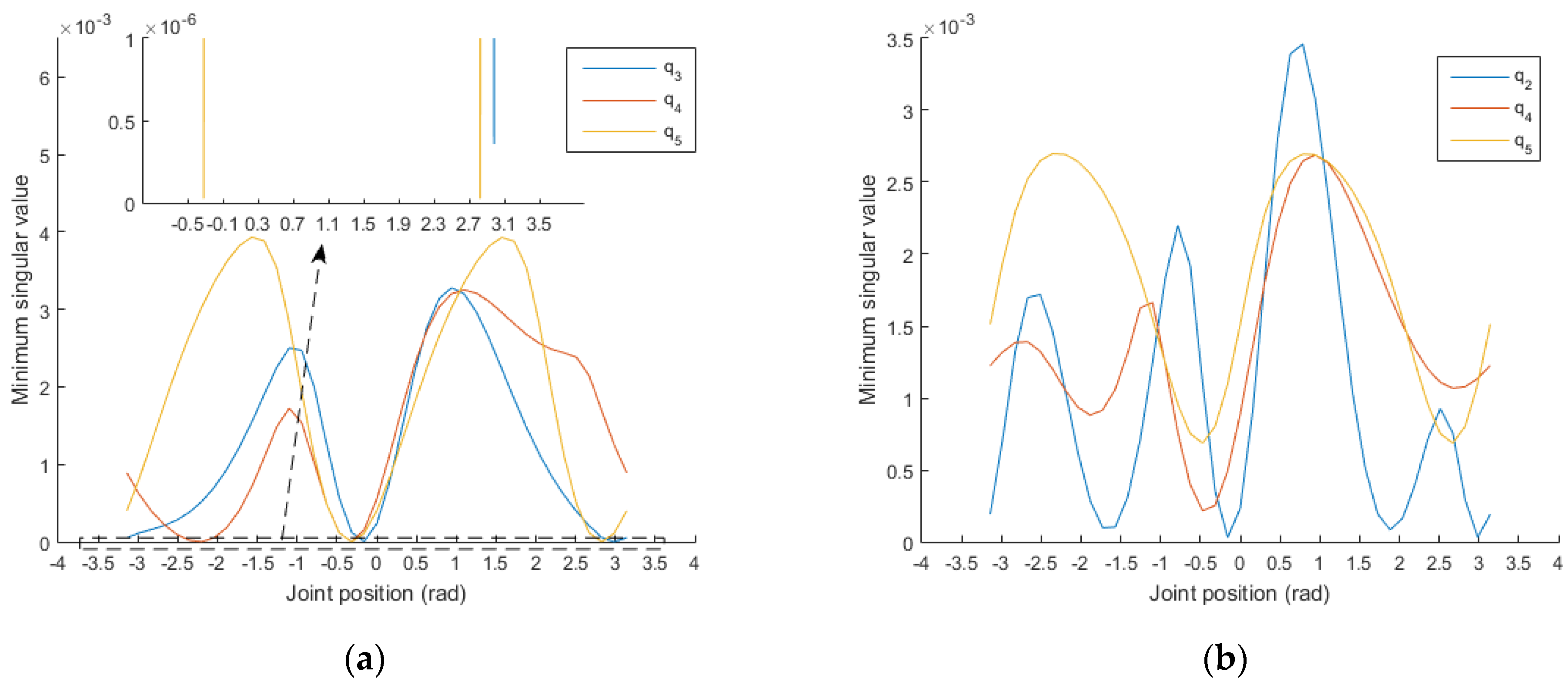
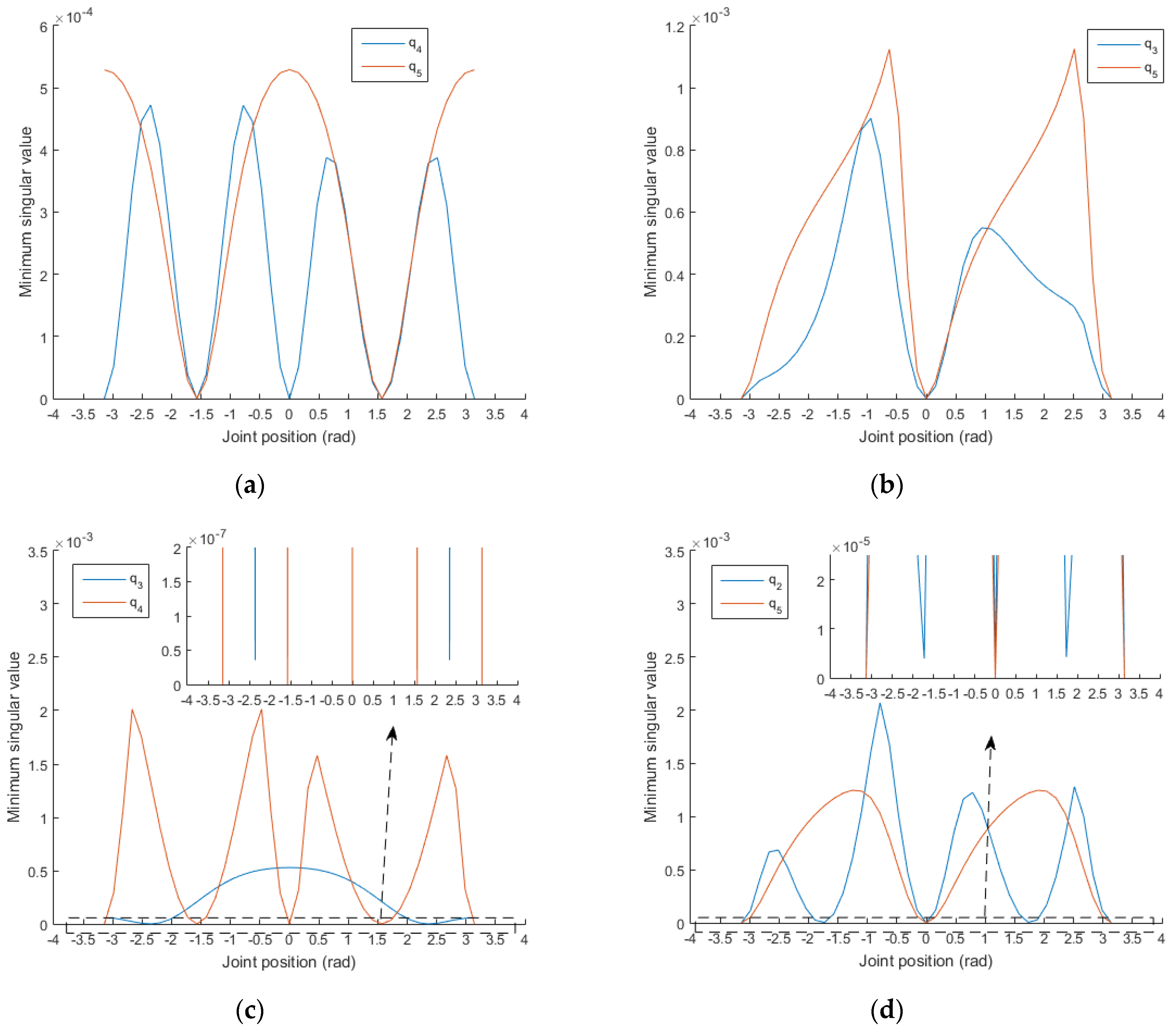
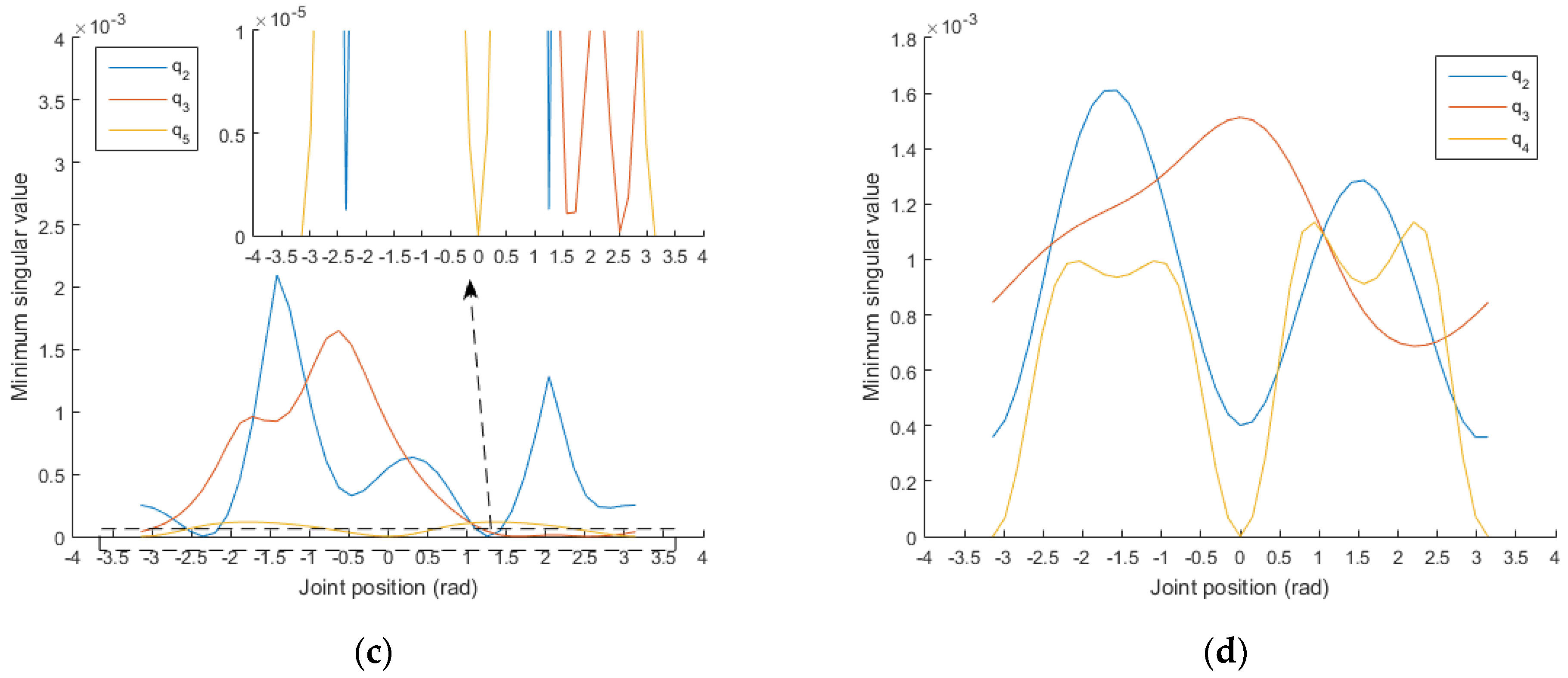
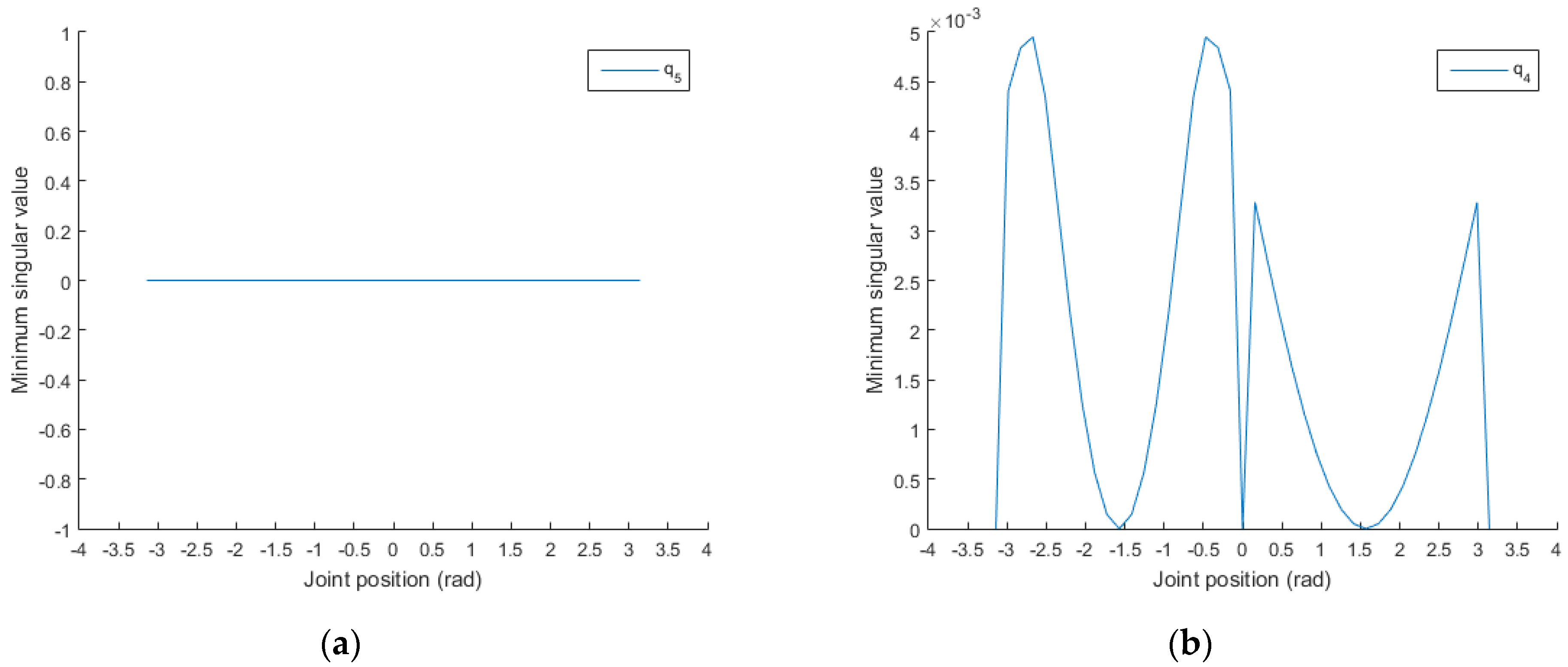
On the basis of the set of joint positions in step 1, two joint positions are selected one by one and set to $0$, $\pm \mathsf{\pi }/2$, $\pm \mathsf{\pi }$. From the remaining joints, a joint is selected and varied within its range, and the other joint positions remain unchanged. Finally, the distribution of the minimum singular value with the change in a joint position is obtained. For example, for a 6-DOF manipulator, $q_1=q_2=0$, $q_4=q_5=q_6=\mathsf{\pi }/3$, and $q_3\in [-\mathsf{\pi },\mathsf{\pi }]$ are set. Finally, the distribution of the minimum singular value with the change in $q_3$ is obtained. In the same way, the distributions of the minimum singular values with the changes in $q_4$, $q_5$, and $q_6$ are also obtained;

(4)

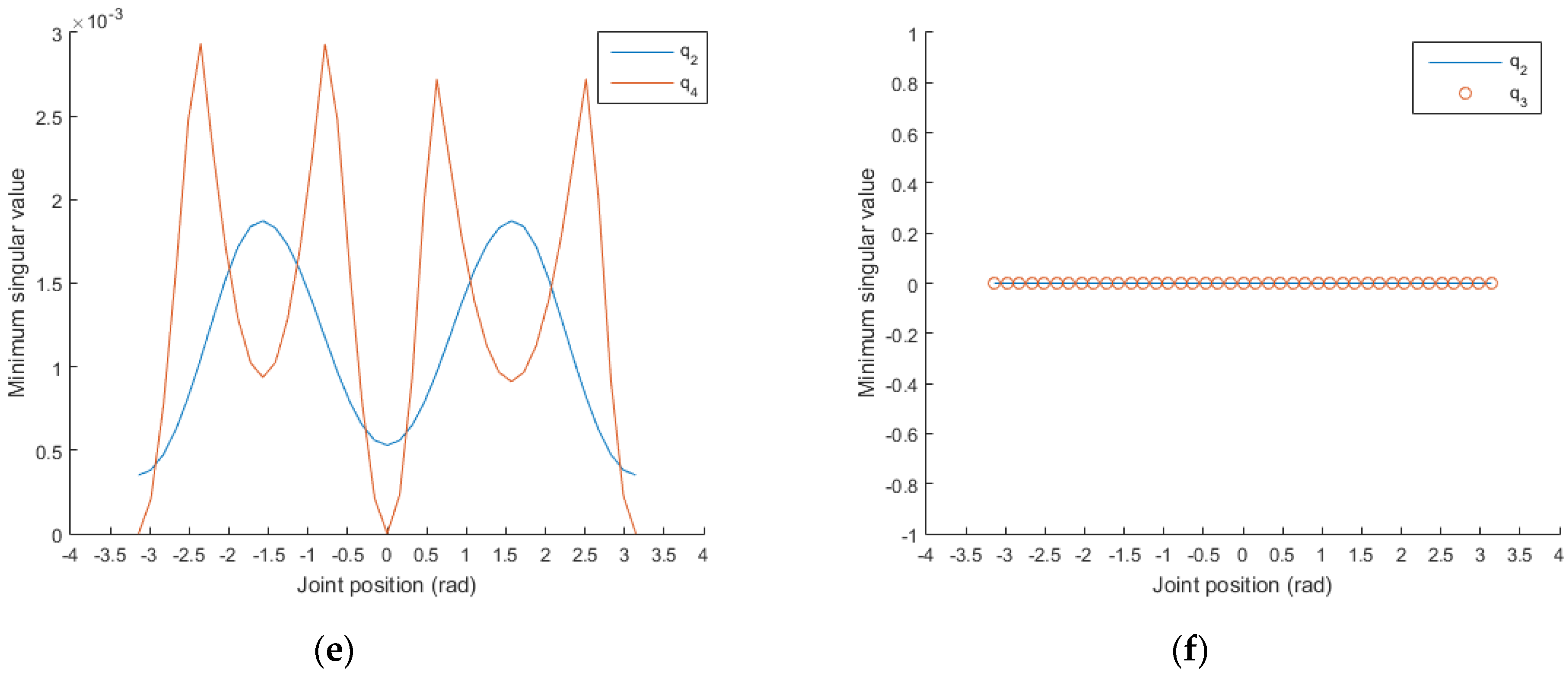
The rest may be deduced by analogy: the distributions of the minimum singular values with the changes in all combined joint positions are obtained. When the minimum singular value is zero, singular configurations occur.

It can be seen that the proposed method does not need to calculate $\det \left(\mathit{J}\right)=0$ to obtain singular configurations. In other words, the proposed method eliminates the more complex mathematical derivation. Especially for redundant manipulators that do not meet the Pieper criterion, it is very difficult to obtain singular configurations through determinant transformation. Fortunately, the minimum singular value distribution curve obtained through the proposed method can clearly show some singular configurations.

3.2.1. Singular Analysis of the Stanford Manipulator Based on the Proposed Method

Analyzing the proposed method steps, in step (1), by setting $q_1=q_2=q_4=q_5=q_6=\mathsf{\pi }/3$ and ${\mathit{d}}_3=0.3$, and by using Equation (7), ${\sigma }_{\min }=0.1447$; this set of joint positions is applied to the subsequent steps in this section.

In step (2), by setting $q_1=q_2=q_4=q_5=q_6=\mathsf{\pi }/2$, ${\mathit{d}}_3=0.3$, and by using Equation (7), ${\sigma }_{\min }=0.209$; this shows that singularity does not occur. Furthermore, by setting $q_1=q_2=q_4=q_5=q_6=0$, $\pm \mathsf{\pi }$, ${\mathit{d}}_3=0.3$, and by using Equation (7), ${\sigma }_{\min }=0$; this shows that singular configurations occur (one or more joints are $0$, $\pm \mathsf{\pi }$). In addition, it can be seen in Figure 2 that the minimum singular value does not change with the change in $q_1$ and $q_6$. Therefore, $q_1$ and $q_6$ can be ignored when using the proposed method to obtain singular configurations.

On the basis of the set of joint positions in step 1, a joint position is selected and set to $0$, $\pm \mathsf{\pi }$ rad. From the remaining joints, a joint is selected and varied within its range, and the other joint positions remain unchanged. The distributions of the minimum singular values with the changes in $q_2$, $q_4$, and $q_5$ can then be obtained, as shown in Figure 3. The distribution of the minimum singular value with the change in ${\mathit{d}}_3$ can also be obtained, as shown in Figure 4.

As only $q_2$, ${\mathit{d}}_3$, $q_4$, and $q_5$ need to be analyzed, there is no need to continue with the subsequent steps of the proposed method. Figure 3 and Figure 4 show that, when $q_2= 0$, $\pm \mathsf{\pi }$; ${\mathit{d}}_3=0$; and $q_5=0$, $\pm \mathsf{\pi }$, singular configurations occur. The results are the same as the singular configurations obtained through the analytical method in Section 3.1. This shows that the proposed method is correct.

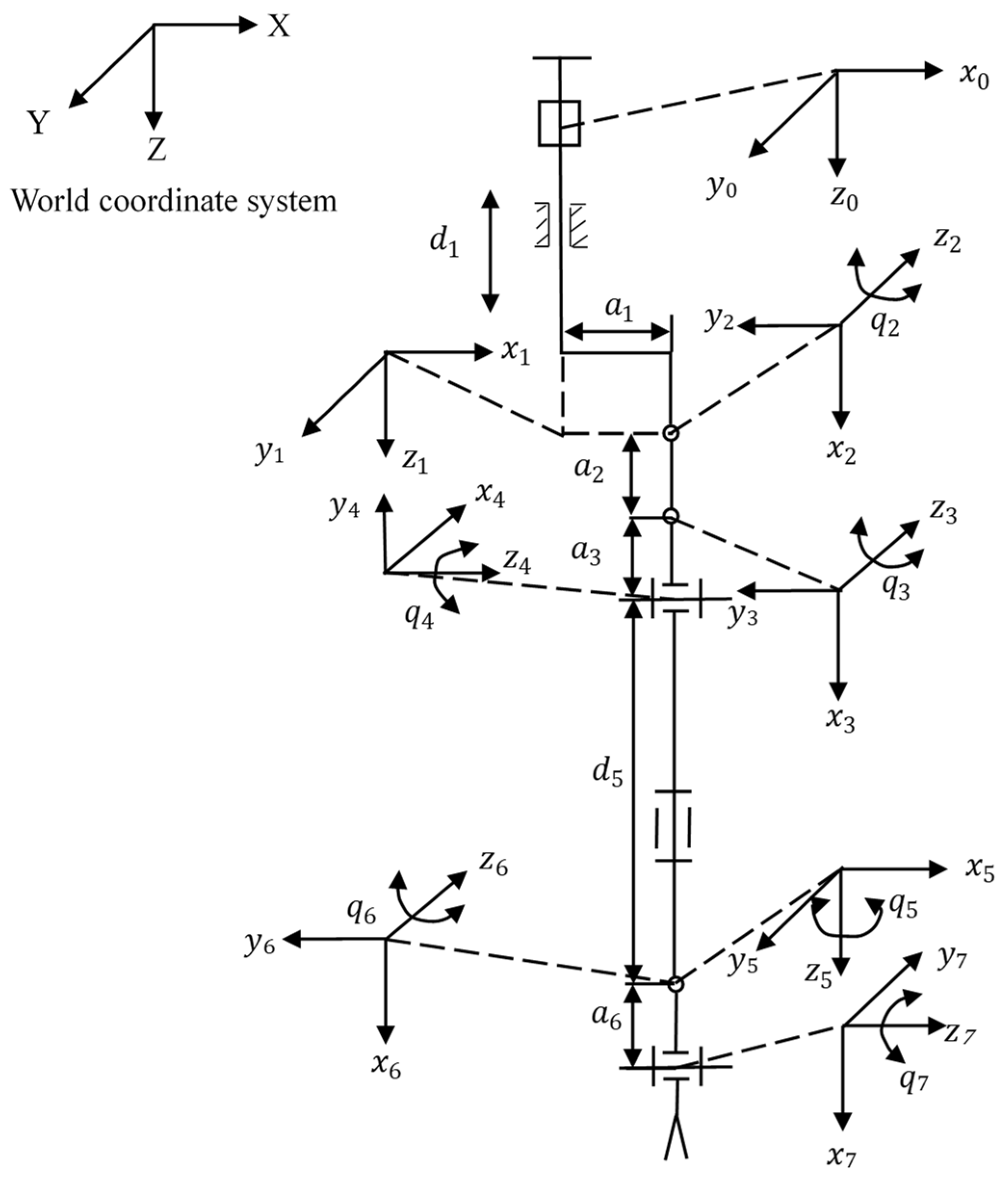
3.2.2. Singular Analysis of a 7-DOF Serial Manipulator Based on the Proposed Method

This section involves a 7-DOF serial manipulator developed by us for laparoscopic surgery that does not meet the Pieper criterion. The coordinate system is established as shown in Figure 5 and the modified DH parameters are shown in

Table 2. Modified DH parameters of the 7-DOF serial manipulator.

i	${\mathit{\alpha }}_{\mathbf{i}} \left(\mathbf{rad}\right)$	${\mathit{a}}_{\mathbf{i}}\left(\mathbf{m}\right)$	${\mathit{d}}_{\mathbf{i}}\left(\mathbf{m}\right)$	${\mathit{q}}_{\mathbf{i}} \left(\mathbf{rad}\right)$	$[{\mathit{q}}_{\mathbf{imin}},{\mathit{q}}_{\mathbf{imax}}]$
1	0	0	${\mathit{d}}_1$	0	$[-0.1,0.1]\left(\mathrm{m}\right)$
2	$\mathsf{\pi }/2$	0.02	0	$q_2$	$[-\mathsf{\pi },\mathsf{\pi }]\left(\mathrm{rad}\right)$
3	0	0.05	0	$q_3$	$[-\mathsf{\pi },\mathsf{\pi }]\left(\mathrm{rad}\right)$
4	$\mathsf{\pi }/2$	0.05	0	$q_4$	$[-\mathsf{\pi },\mathsf{\pi }]\left(\mathrm{rad}\right)$
5	$\mathsf{\pi }/2$	0	0.1	$q_5$	$[-\mathsf{\pi },\mathsf{\pi }]\left(\mathrm{rad}\right)$
6	$\mathsf{\pi }/2$	0	0	$q_6$	$[-\mathsf{\pi },\mathsf{\pi }]\left(\mathrm{rad}\right)$
7	$\mathsf{\pi }/2$	0.02	0	$q_7$	$[-\mathsf{\pi },\mathsf{\pi }]\left(\mathrm{rad}\right)$

.

According to the proposed method steps, in step (1), by setting $q_2=q_3=q_4=q_5=q_6=q_7=\mathsf{\pi }/3$ and ${\mathit{d}}_1=0.3$, and by using Equation (8), ${\sigma }_{\min }=0.000472$; this set of joint positions is applied to the subsequent steps in this section.

In step (2), by setting $q_2=q_3=q_4=q_5=q_6=q_7=\mathsf{\pi }/2$ and ${\mathit{d}}_1=0.3$, and by using Equation (8), ${\sigma }_{\min }=0.000442$; this shows that singularity does not occur when all joint positions are $\mathsf{\pi }/2$. Furthermore, by setting $q_2=q_3=q_4=q_5=q_6=q_7=0$, $\pm \mathsf{\pi }$ and ${\mathit{d}}_1=0.3$, and by using Equation (8), ${\sigma }_{\min }=0$; this shows that singular configurations occur (one or more joints are $0$, $\pm \mathsf{\pi }$). In addition, it is found that the minimum singular value does not change with the change of ${\mathit{d}}_1$ and $q_7$ through Figure 6. Also, the order of magnitude of the minimum singular value varying with $q_6$ is 10⁻⁶. Therefore, ${\mathit{d}}_1$, $q_6$, and $q_7$ can be ignored when using the proposed method to obtain singular configurations.

On the basis of the set of joint positions in step 1, a joint position is selected and set to $0$, $\pm \mathsf{\pi }$ rad. From the remaining joints, a joint is selected and varied within its range, and the other joint positions remain unchanged. The distributions of the minimum singular values with the changes in $q_2$, $q_3$, $q_4$, and $q_5$ can then be obtained, as shown in Figure 7.

In step (3), on the basis of the set of joint positions in step 1, two joint positions are selected one by one and set to $0$, $\pm \mathsf{\pi }$ rad. From the remaining joints, a joint is selected and varied within its range, and the other joint angles remain unchanged. The distributions of the minimum singular values with the changes in $q_2$, $q_3$, $q_4$, and $q_5$ can then be obtained, as shown in Figure 8.

In step (4), on the basis of the set of joint positions in step 1, three joint positions are selected one by one and set to $0$, $\pm \mathsf{\pi }$ rad. From the remaining joints, a joint is selected and varied within its range, and the other joint angles remain unchanged. The distributions of the minimum singular values with the changes in $q_4$ and $q_5$ can then be obtained, as shown in Figure 9.

Figure 7, Figure 8 and Figure 9 show that when $q_2=q_3=q_4=0$, $\pm \mathsf{\pi }$; $q_2=q_3=0$, $\pm \mathsf{\pi }$, and $q_5=\pm \mathsf{\pi }/2$; $q_4=q_5=0$, $\pm \mathsf{\pi }$, singular configurations occur.

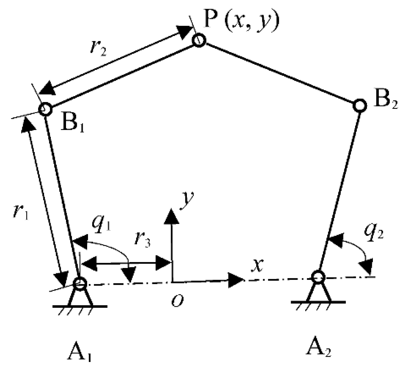
3.2.3. Singular Analysis of a Planar 5R Parallel Robot Based on the Proposed Method

To verify that the proposed method is also suitable for parallel manipulators, a planar 5R parallel manipulator [28] was taken as an example for analysis. The mechanism diagram is shown in Figure 10. ${\mathrm{A}}_1$ and ${\mathrm{A}}_2$ represent the drive pair, and the other end of the drive link is represented by ${\mathrm{B}}_1$ and ${\mathrm{B}}_2$. The common intersection point of the two branch chains is represented by $\mathrm{P}(x,y)$ as the output point. The origin of the coordinate system is at the center of ${\mathrm{A}}_1{\mathrm{A}}_2$, x is along the direction of ${\mathrm{A}}_1{\mathrm{A}}_2$, and the y-axis is perpendicular to ${\mathrm{A}}_1{\mathrm{A}}_2$. $O{\mathrm{A}}_1=O{\mathrm{A}}_2$ and ${\mathrm{PB}}_1={\mathrm{PB}}_2$. Under the premise that the output pose is $\mathit{X}$ and the drive is $\mathit{q}$, the robot’s input–output relationship is:

$$f(\mathit{q},\mathit{X})=0$$

(12)

The relationship on the velocity level is as follows [29]:

$${\mathit{J}}_{\mathit{x}} \dot{\mathit{X}} +{\mathit{J}}_q \dot{\mathit{q}} =0$$

(13)

where ${\mathit{J}}_{\mathit{x}}=\left[\begin{array}{cc}y\cos q_1-(x+r_3)\sin q_1& 0\\ 0& y\cos q_2+(-x+r_3)\sin q_2\end{array}\right]\ast r_1$ is the configuration Jacobian matrix and ${\mathit{J}}_q=\left[\begin{array}{cc}x+r_3-r_1\cos q_1& y-r_1\sin q_1\\ x-r_3-r_1\cos q_2& y-r_1\sin q_2\end{array}\right]$ is the mechanism Jacobian matrix. $e=\frac{r_1(\sin q_1-\sin q_2)}{2r_3+r_1\cos q_2-r_1\cos q_1}$, $f=\frac{r_1{r}_3(\cos q_1+\cos q_2)}{2r_3+r_1\cos q_2-r_1\cos q_1}$, $d=1+e^2$, $g=2(ef-e{r}_1\cos q_1+e{r}_3-r_1\sin q_1)$, $h=f^2-2f(r_1\cos q_1-r_3)-2r_1{r}_3\cos q_1+r_3^2+r_1^2-r_2^2$, $x=ey+f$, $y=\frac{\sqrt{g^2-4dh}-g}{2d}$, ${\mathrm{A}}_1{\mathrm{B}}_1={\mathrm{A}}_2{\mathrm{B}}_2=r_1=1.2 \mathrm{m}$, ${\mathrm{B}}_1\mathrm{P}={\mathrm{B}}_2\mathrm{P}=r_2=1 \mathrm{m}$, $\mathrm{O}{\mathrm{A}}_1=r_3=0.8 \mathrm{m}$.

We can analyze the configuration Jacobian matrix according to the proposed method steps. In step (1), by setting $q_1=\mathsf{\pi }/3$,$q_2=\mathsf{\pi }/3$, and by using Equation (8), ${\sigma }_{\min }=0.4714$; this set of joint positions is applied to the subsequent steps in this section. In step (2), on the basis of the set of joint positions in step 1, a joint position is selected and set to $\mathsf{\pi }/3$ rad. From the remaining joints, a joint is selected and varied within its range, and the other joint positions remain unchanged. The distributions of the minimum singular values with the changes in $q_1$ and $q_2$ can then be obtained, as shown in Figure 11a.

We can also analyze the mechanism Jacobian matrix according to the proposed method steps. In step (1), by setting $q_1=\mathsf{\pi }/3$,$q_2=\mathsf{\pi }/3$, and by using Equation (8), ${\sigma }_{\min }=0.8485$; this set of joint positions is applied to the subsequent steps in this section. In step (2), on the basis of the set of joint positions in step 1, a joint position is selected and set to $\mathsf{\pi }/3$ rad. From the remaining joints, a joint is selected and varied within its range, and the other joint positions remain unchanged. The distributions of the minimum singular values with the changes in $q_1$ and $q_2$ can then be obtained, as shown in Figure 11b. It can be seen that there is no mechanism singularity and when $q_1=\mathsf{\pi }/3 \mathrm{rad}{, q}_2=1.40924 \mathrm{rad}$; $q_1=\mathsf{\pi }/3 \mathrm{rad}{, q}_2=2.70535 \mathrm{rad}$; $q_1=\mathsf{\pi }/3 \mathrm{rad}{, q}_2=1.96856 \mathrm{rad}$; and $q_1=0.86476 \mathrm{rad}{, q}_2=\mathsf{\pi }/3 \mathrm{rad}$, internal singularities appear.

4. Method Verification

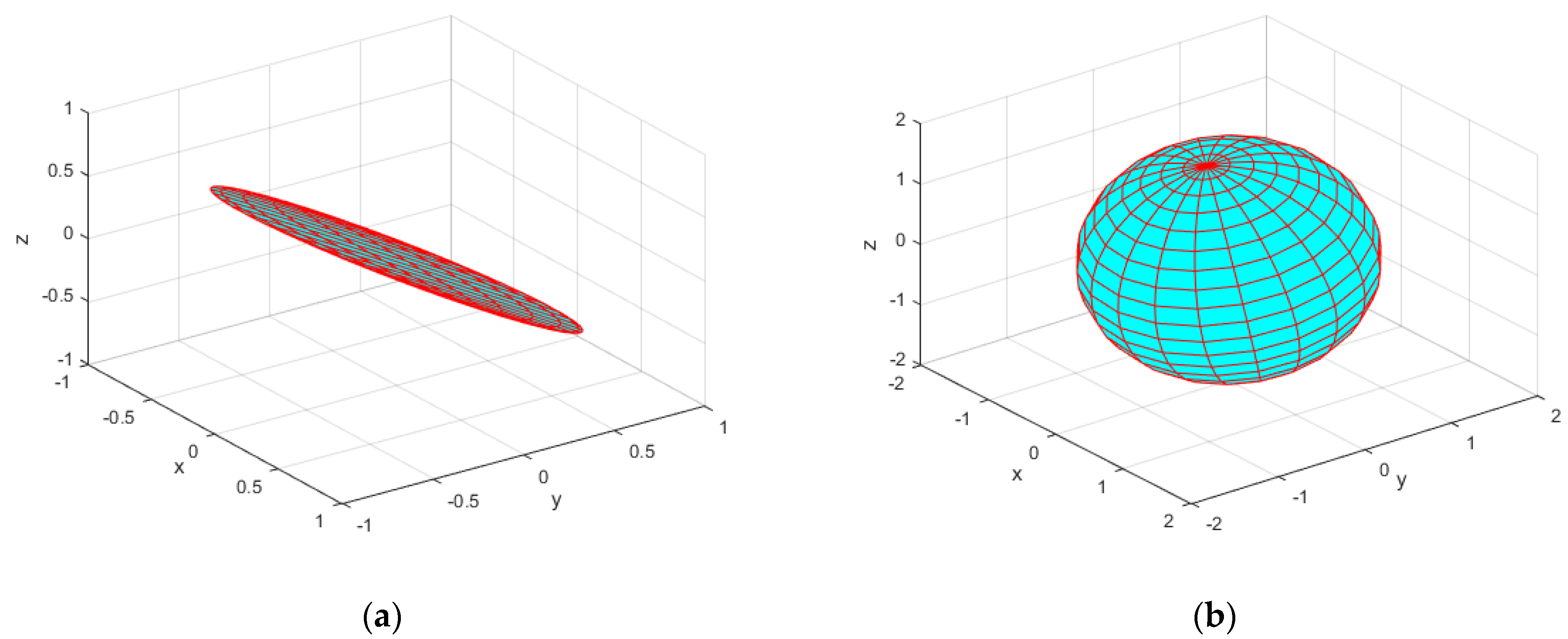
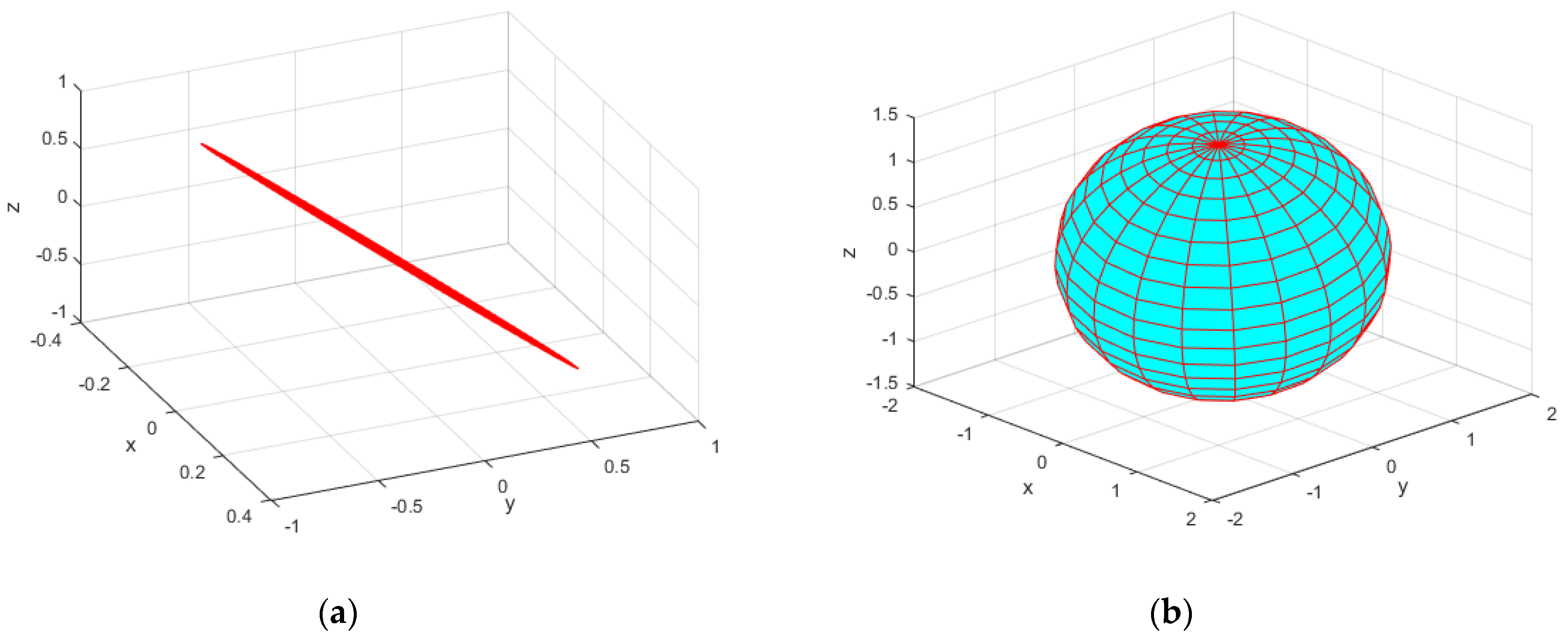
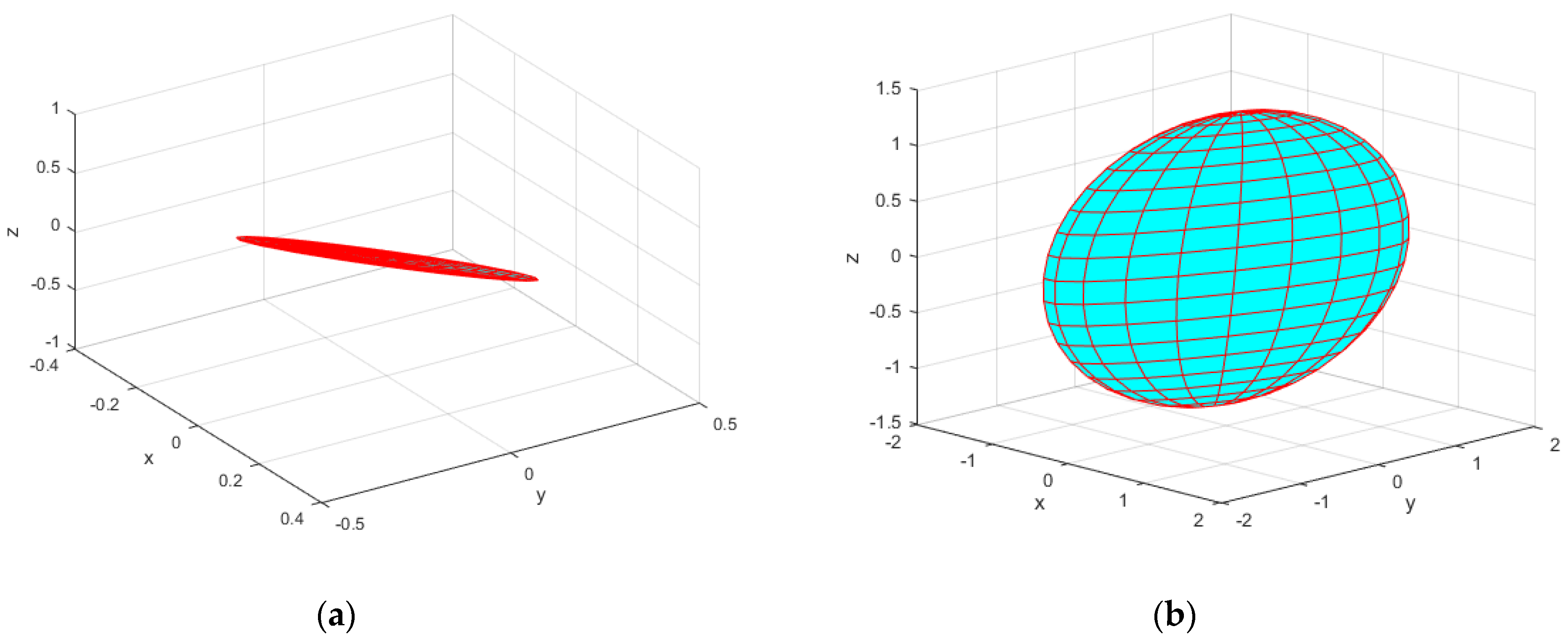
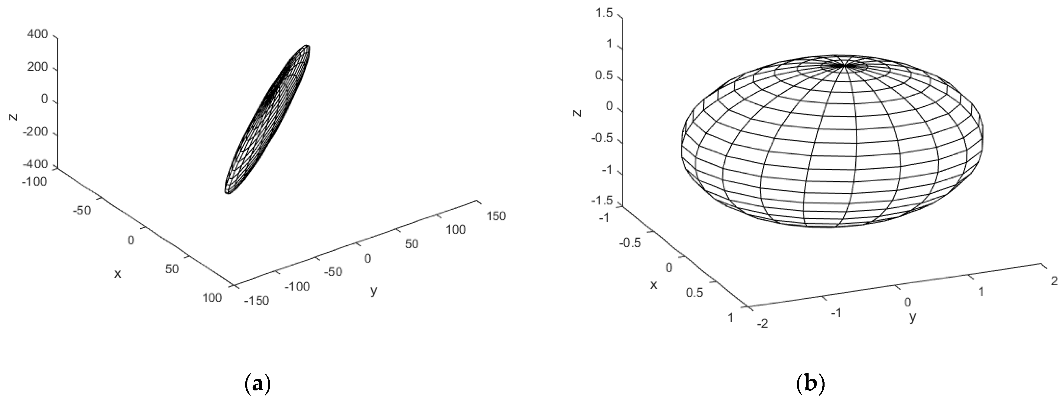
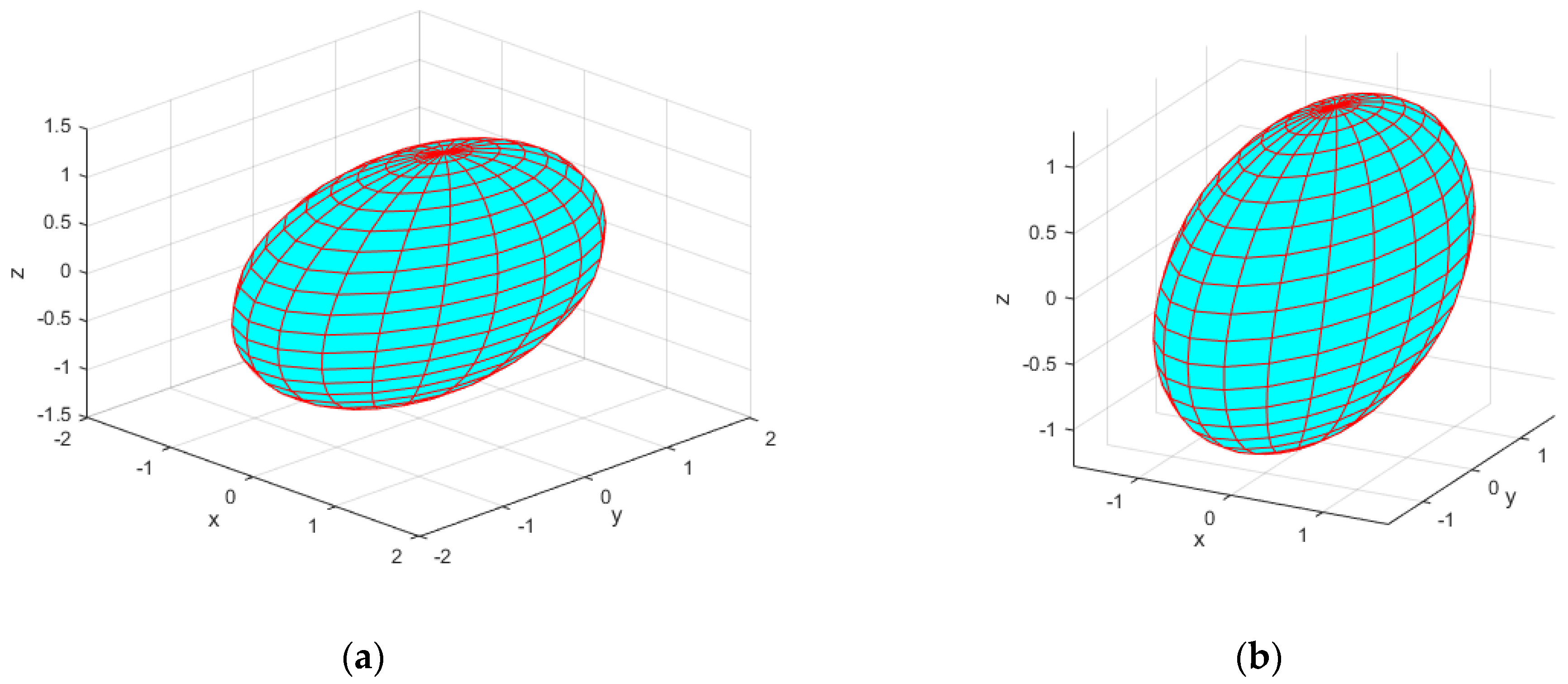
4.1. Singularity Configurations of the 7-DOF Serial Manipulator Verified through the EE Velocity Ellipsoid

The flexibility of robotic manipulators is the key aspect of research in kinematics, and the manipulability measure is an evaluable index. Yoshikawa [30] defined the manipulability measure as follows:

$$\omega (\mathit{q})=\sqrt{\det ({\mathit{JJ}}^{\mathrm{T}})}$$

(14)

Corke [31] further proposed the EE velocity ellipsoid on the basis of the manipulability measure, as shown in Figure 12. This ellipsoid describes the flexibility of robotic manipulators’ motion at the geometric level more vividly, and it defines the joint velocities of robotic manipulators as a unit sphere; i.e.,

$${\Vert \dot{\mathit{q}}\Vert }^2={\dot{q}}_1^2+{\dot{q}}_2^2+\cdot \cdot \cdot +{\dot{q}}_n^2\le 1$$

(15)

where n represents the number of joints. ${\Vert \dot{\mathit{q}}\Vert }^2$ is mapped to the ellipsoid of the task space through the Jacobian matrix $\mathit{J}$; i.e.,

$${ \dot{\mathit{x}} }^{\mathrm{T}}{({\mathit{JJ}}^{\mathrm{T}})}^{-1} \dot{\mathit{x}} \le 1$$

(16)

The direction of each axis of the ellipsoid is consistent with the eigenvector of ${({\mathit{JJ}}^{\mathrm{T}})}^{-1}$. The length of each axis is equal to the reciprocal of the square root of its eigenvalue, and it is also equal to the singular value of $\mathit{J}$. When robotic manipulators approach a singular configuration, $\omega (\mathit{q})=0$ and the elliptical plate has almost zero thickness [31].

The translational velocity ellipsoid and rotational velocity ellipsoid of the EE corresponding to the singular configurations of the 7-DOF serial manipulator obtained in Section 3.2.2 are shown in Figure 13, Figure 14 and Figure 15. To illustrate the singular configurations, the 7-DOF serial manipulator is returned to a nominal configuration and the corresponding translational velocity and rotational velocity ellipsoids are computed, as shown in the Figure 16. Figure 16 clearly indicates that the EE translational velocity and rotational velocity ellipsoids are both standard ellipsoids. However, Figure 13b, Figure 14b and Figure 15b illustrate that the translational velocity ellipse evolves into an elliptical plate with a thickness of zero, indicating that the manipulability measure of the 7-DOF serial manipulator is zero, i.e., the 7-DOF serial manipulator approaches singular configurations. It is thus verified that the singular configurations of the 7-DOF serial manipulator obtained by the proposed method are correct.

4.2. Singularity Configurations of the 7-DOF Serial Manipulator and the Planar 5R Parallel Manipulator Verified through an Analytical Method

In Equation (6), ${\sigma }_1$ and ${\sigma }_{\mathrm{r}}$ are the maximum and minimum singular values, respectively. The condition number is defined as follows [32]:

$$K\left(\mathit{q}\right)=\frac{{\sigma }_1}{{\sigma }_{\mathrm{r}}}$$

(17)

It is used to define whether a Jacobian matrix is “good” or “ill-conditioned”. When $K(\mathit{q})=1$, the flexibility of the manipulator’s movement is optimal. When $K\left(\mathit{q}\right)$ is infinite, the manipulator is in a singular configuration.

For the 7-DOF serial manipulator, the values for $\det (\mathit{J}(\mathit{q}))$, $\omega (\mathit{q})$, and $K\left(\mathit{q}\right)$ corresponding to the singular configurations obtained through the proposed method can be calculated using Equations (5), (14), and (17), as shown in

Table 3. $\det (\mathit{J}(\mathit{q}))$, $\omega (\mathit{q})$, and $K\left(\mathit{q}\right)$ with singularity and approximate singularity.

Joint Position	$\mathbf{det}(\mathit{J}(\mathit{q}))$	$\mathit{\omega }(\mathit{q})$	$\mathit{K}\left(\mathit{q}\right)$
${\mathit{d}}_1=0.3, q_2=q_3=q_4=0 (\pm \mathsf{\pi }),q_5=q_6=q_7=\mathsf{\pi }/3$	0	0	$\infty$
${\mathit{d}}_1=0.3, q_5=q_4=0 (\pm \mathsf{\pi }), q_2=q_3=q_6=q_7=\mathsf{\pi }/3$	0	0	$\infty$
${\mathit{d}}_1=0.3, q_2=q_3=0 (\pm \mathsf{\pi }),q_5=\pm \mathsf{\pi }/2{, q}_4=q_6=q_7=\mathsf{\pi }/3$	0	0	$\infty$
${\mathit{d}}_1=0.3, q_2=0 (\pm \mathsf{\pi }){, q}_3=-0.1571, q_4={ q}_5=q_6=q_7=\mathsf{\pi }/3$	0.00000027	0.000523	613,002
${\mathit{d}}_1=0.3, q_2=0 (\pm \mathsf{\pi }){, q}_3=2.9845, q_4={ q}_5=q_6=q_7=\mathsf{\pi }/3$	0.00000000215	0.0000464	8,500,392
${\mathit{d}}_1=0.3, q_2=0 (\pm \mathsf{\pi }){, q}_4=-0.3142, q_3={ q}_5=q_6=q_7=\mathsf{\pi }/3$	0.0000000248	0.0001575	4,423,851
${\mathit{d}}_1=0.3, q_2=0 (\pm \mathsf{\pi }){, q}_5=-0.3142, q_3={ q}_4=q_6=q_7=\mathsf{\pi }/3$	0.00000000147	0.0000383	113,310,832
${\mathit{d}}_1=0.3, q_4=0 (\pm \mathsf{\pi }){, q}_2=-2.3562, q_3={ q}_5=q_6=q_7=\mathsf{\pi }/3$	0.0000000463	0.000215	2,410,219
${\mathit{d}}_1=0.3, q_4=0 (\pm \mathsf{\pi }){, q}_2=1.2566, q_3={ q}_5=q_6=q_7=\mathsf{\pi }/3$	0.0000000324	0.00018	2,364,066
${\mathit{d}}_1=0.3, q_4=0 (\pm \mathsf{\pi }){, q}_3=1.5708, q_2={ q}_5=q_6=q_7=\mathsf{\pi }/3$	0.0000000155	0.0001246	2,777,778
${\mathit{d}}_1=0.3, q_4=0 (\pm \mathsf{\pi }){, q}_3=2.513, q_2={ q}_5=q_6=q_7=\mathsf{\pi }/3$	0.000000001	0.0000314	20,703,933
${\mathit{d}}_1=0.3{, q}_2=q_5=0 (\pm \mathsf{\pi }),q_3=\pm 2.3562, q_4=q_6=q_7=\mathsf{\pi }/3$	0.000000001	0.0000308	77,294,250
${\mathit{d}}_1=0.3, q_3=q_4=0 (\pm \mathsf{\pi }),q_2=\pm 1.7279 ,q_5=q_6=q_7=\mathsf{\pi }/3$	0.0000002081	0.000456	705,496

. It can be seen that the corresponding values for $\det (\mathit{J}(\mathit{q}))$ and $\omega (\mathit{q})$ for the first to the third rows are zero, and the corresponding values for $K\left(\mathit{q}\right)$ tend to infinity. This further indicates that the singular configurations obtained by the proposed method are correct. In addition, $\det (\mathit{J}(\mathit{q}))$ and $\omega (\mathit{q})$ for the fourth to the thirteenth row are near zero, and the corresponding values for $K\left(\mathit{q}\right)$ are very large. The larger the $K\left(\mathit{q}\right)$, the closer the configuration is to a singular configuration. This indicates that the flexibility of the manipulator is very poor, so configurations with singular values of zero or approximately zero should be avoided in the actual motion of robotic manipulators.

Furthermore, for the planar 5R parallel manipulator, the values for $\det (\mathit{J}(\mathit{q}))$, $\omega (\mathit{q})$, and $K\left(\mathit{q}\right)$ corresponding to the singular configurations obtained through the proposed method can be calculated using Equations (5), (14) and (17), as shown in

Table 4. $\det (\mathit{J}(\mathit{q}))$, $\omega (\mathit{q})$, and $K\left(\mathit{q}\right)$ with singularity.

Joint Position	$\mathbf{det}(\mathit{J}(\mathit{q}))$	$\mathit{\omega }(\mathit{q})$	$\mathit{K}\left(\mathit{q}\right)$
$q_1=\mathsf{\pi }/3 ,q_2=1.40924$	0	0	$\infty$
$q_1=\mathsf{\pi }/3 ,q_2=2.70535$	0	0	$\infty$
$q_1=\mathsf{\pi }/3 ,q_2=1.96856$	0	0	$\infty$
$q_1=0.86476 ,q_2=\mathsf{\pi }/3$	0	0	$\infty$

. It can be seen that the corresponding values for $\det (\mathit{J}(\mathit{q}))$ and $\omega (\mathit{q})$ are zero, and the corresponding values for $K\left(\mathit{q}\right)$ tend to infinity. This further indicates that the singular configurations obtained by the proposed method are correct.

Finally, the proposed method is compared with the analytical method in terms of three aspects: the complexity of the determinant transformation, whether they are able to solve $\det (\mathit{J}(\mathit{q}))=0$, and whether they are able to obtain singular configurations, as shown in

Table 5. Results for the proposed method.

Manipulator Type	The Complexity of Determinant Transformation	$\mathbf{Capable} \mathbf{of} \mathbf{Solving} \mathbf{det}(\mathit{J}(\mathit{q}))=0$	Capable of Obtaining Singular Configurations
Serial manipulators satisfying the Pieper criterion	No determinant transformation	No	Yes
Serial manipulators not satisfying the Pieper criterion	No determinant transformation	No	Yes
Parallel manipulators	No determinant transformation	No	Yes

and

Table 6. Results for the analytical method.

Manipulator Type	The Complexity of Determinant Transformation	$\mathbf{Capable} \mathbf{of} \mathbf{Solving} \mathbf{det}(\mathit{J}(\mathit{q}))=0$	Capable of Obtaining Singular Configurations
Serial manipulators satisfying the Pieper criterion	Average complexity	Yes	Yes
Serial manipulators not satisfying the Pieper criterion	Very complex	Yes	No
Parallel manipulators	Average complexity	Yes	Yes

. The results show that the proposed method can obtain some singular configurations of serial manipulators and parallel manipulators and that it is able to eliminate complex determinant transformation and obtain the solution of $\det (\mathit{J}(\mathit{q}))=0$.

5. Conductions and Future Work

For serial manipulators that do not meet the Pieper criterion, it is difficult to obtain singular configurations through the analytical method. A joint angle parameterization method to be used to obtain singular configurations for robotic manipulators was here proposed. First, an analytical method was used to analyze singular configurations of the Stanford manipulator. Then, the singular configurations of the Stanford manipulator were obtained through the proposed method and compared with the results obtained with the analytical method. The correctness of the proposed method was verified. Next, the proposed method was applied to a 7-DOF serial manipulator and a planar 5R parallel manipulator. Finally, the translational velocity ellipsoid of the EE under singular configurations of the 7-DOF serial manipulator obtained through the proposed method was found to be a plane, and the values for $\det (\mathit{J}(\mathit{q}))=0$, $\omega (\mathit{q})=0$, and $K\left(\mathit{q}\right)\to \infty$ corresponding to singular configurations were calculated. The correctness of the proposed method was verified from these two aspects. For the planar 5R parallel manipulator, by calculating the values for $\det (\mathit{J}(\mathit{q}))=0$, $\omega (\mathit{q})=0$, and $K\left(\mathit{q}\right)\to \infty$ corresponding to singular configurations, the correctness of the proposed method was verified. This showed that the proposed method can be applied to both serial manipulators and parallel manipulators and that it can eliminate complex determinant transformation and obtain the solution of $\det (\mathit{J}(\mathit{q}))=0$.

The proposed method can only obtain singular configurations of robotic manipulators at a specific angle, but cannot obtain singular configurations of multiple angles satisfying a certain equation. For example, one singular configuration of PUMA 560 is ${\mathit{d}}_4\sin (q_2+q_3)+{\mathrm{a}}_2\cos (q_2)+{\mathrm{a}}_3\cos (q_2+q_3)=0$, and one singular configuration of ABB IRB 1400 is ${\mathrm{a}}_3\sin (q_2+q_3)-d_4\cos (q_2+q_3)+{\mathrm{a}}_2\sin (q_2)-{\mathrm{a}}_1=0$. As there are countless combination angles satisfying these two equations, the proposed method fails. Although the proposed method cannot be guaranteed to find all singular configurations, in reality, singular configurations obtained with the proposed method can be set in the initial parameters of manipulators to avoid the corresponding configurations, which is similar to avoiding predetermined fixed obstacles in the working environment. Otherwise, these singular configurations can only be solved by the singularity avoidance algorithm, which reduces the pose accuracy of the EE and makes the calculation more complex. In addition, in the fourth to thirteenth rows of Table 3 (as a few examples; in fact, there are many similar situations), the determinants and the manipulability measures are near zero, and the corresponding condition numbers are very large. In these cases, the velocities of some joints are also very high, which can seriously affect the motion performance. We plan to solve the problem of joint velocities caused by these two situations using a damped least square algorithm in the future. On this basis, we will continue to work on inverse kinematics analysis and trajectory planning.

References

- Peiper, D.L. The Kinematics of Manipulators under Computer Control; Stanford University: Stanford, CA, USA, 1968. [Google Scholar]
- Craig, J.J. Introduction to Robotics: Mechanics and Control; Stanford University: Stanford, CA, USA, 2018; pp. 105–108. [Google Scholar]
- Merlet, J.P. Parallel Robots; Springer: Dordrecht, The Netherlands, 2006; pp. 179–213. [Google Scholar]
- Müller, A. Local Analysis of Singular Configurations of Open and Closed Loop Manipulators. Multibody Syst. Dyn. 2002, 8, 299–328. [Google Scholar] [CrossRef]
- Li, C.Y.; Angeles, J.; Guo, H.W. Mobility and singularity analyses of a symmetric multi-loop mechanism for space applications. Proc. Inst. Mech. Eng. C. J. Mech. Eng. Sci. 2021. [Google Scholar] [CrossRef]
- Han, J.Y.; Shi, S.J. A novel methodology for determining the singularities of planar linkages based on Assur groups. Mech. Mach. Theory 2020, 147, 103751. [Google Scholar] [CrossRef]
- Chen, Z.M.; Li, M.; Kong, X.W.; Zhao, C. Kinematics analysis of a novel 2R1T 3-PUU parallel mechanism with multiple rotation centers. Mech. Mach. Theory 2020, 152, 103938. [Google Scholar] [CrossRef]
- Nayak, A.; Caro, S.; Wenger, P. Kinematic analysis of the 3-RPS-3-SPR series-parallel manipulator. Robotica. 2019, 37, 1240–1266. [Google Scholar] [CrossRef] [Green Version]
- Ma, J.Y.; Chen, Q.H.; Yao, H.J.; Chai, X.X.; Li, Q.C. Singularity analysis of the 3/6 Stewart parallel manipulator using geometric algebra. Math. Method. Appl. Sci. 2018, 41, 2494–2506. [Google Scholar] [CrossRef]
- Wu, X.Y.; Bai, S.P. Analytical determination of shape singularities for three types of parallel manipulators. Mech. Mach. Theory 2020, 149, 103812. [Google Scholar] [CrossRef]
- Ben-Horin, P.; Shoham, M. Application of Grassmann—Cayley Algebra to Geometrical Interpretation of Parallel Robot Singularities. Int. J. Robot. Res. 2009, 28, 127–141. [Google Scholar] [CrossRef]
- Conconi, M.; Carricato, M. A New Assessment of Singularities of Parallel Kinematic Chains. IEEE. T. Robot. 2009, 25, 757–770. [Google Scholar] [CrossRef]
- Pagis, G.; Bouton, N.; Briot, S.; Martinet, P. Enlarging parallel robot workspace through Type-2 singularity crossing. Control Eng Pract. 2015, 39, 1–11. [Google Scholar] [CrossRef] [Green Version]
- Li, X.H.; Sheng, R.; Zhang, L.G.; Song, T.; Zhang, J. Singular Configuration Analysis of 6-DOF Modular Manipulator. Tran. Chin. Soc. Agric. Mach. 2017, 7, 376–382. [Google Scholar]
- Yu, T.; Wang, D.; Gao, L. Singularity avoidance for manipulators with spherical wrists using the approximate damped reciprocal algorithm. Int. J. Adv. Robot. Syst. 2021, 18, 172988142199568. [Google Scholar] [CrossRef]
- Carmichael, M.G.; Liu, D.; Waldron, K.J. A framework for singularity-robust manipulator control during physical human-robot interaction. Int. J. Robot. Res. 2017, 36, 027836491769874. [Google Scholar] [CrossRef] [Green Version]
- Kang, Z.H.; Cheng, C.A.; Huang, H.P. A singularity handling algorithm based on operational space control for six-degree-of-freedom anthropomorphic manipulators. Int. J. Adv. Robot. Syst. 2019, 16, 172988141985891. [Google Scholar] [CrossRef] [Green Version]
- Xu, W.F.; Zhang, J.T.; Liang, B.; Li, B. Singularity Analysis and Avoidance for Robot Manipulators with Non-spherical Wrists. IEEE Trans. Ind. Electron. 2016, 63, 277–290. [Google Scholar] [CrossRef]
- Hijazi, A.; Brethé, J.F.; Lefebvre, D. Singularity analysis of a planar robotic manipulator: Application to an XY-Theta platform. Mech. Mach. Theory 2016, 100, 104–119. [Google Scholar] [CrossRef]
- Müller, A. Higher-Order Analysis of Kinematic Singularities of Lower Pair Linkages and Serial Manipulators. J. Mech. Robot. 2018, 10, 011008. [Google Scholar] [CrossRef]
- Oetomo, D.; Ang, M.H., Jr. Singularity robust algorithm in serial manipulators. Robot Comput. Integr. Manuf. 2009, 25, 122–134. [Google Scholar] [CrossRef]
- Rebouças Filho, P.P.; da Silva, S.P.; Praxedes, V.N.; Hemanth, J.; de Albuquerque, V.H.C. Control of singularity trajectory tracking for robotic manipulator by genetic algorithms. J. Comput. Sci. 2019, 30, 55–64. [Google Scholar] [CrossRef]
- Wang, X.H.; Zhang, D.W.; Zhao, C.; Zhang, H.Y.; Yan, H.L. Singularity analysis and treatment for a 7R 6-DOF painting robot with non-spherical wrist. Mech. Mach. Theory 2018, 126, 92–107. [Google Scholar] [CrossRef]
- Dimeas, F.; Moulianitis, V.C.; Aspragathos, N. Manipulator performance constraints in human-robot cooperation. Robot. Comput. Integr. Manuf. 2017, 50, 222–233. [Google Scholar] [CrossRef]
- Wu, J.; Deer, B.; Feng, X.; Wen, Z.; Yin, Z. GA based adaptive singularity-robust path planning of space robot for on-orbit detection. Complexity 2018, 6, 1–11. [Google Scholar] [CrossRef]
- Li, T.; Pei, L.; Xiang, Y.; Wu, Q.; Yu, W. P3-LOAM: PPP/LiDAR Loosely Coupled SLAM with Accurate Covariance Estimation and Robust RAIM in Urban Canyon Environment. IEEE Sens. J. 2020, 21, 6660–6671. [Google Scholar] [CrossRef]
- Huo, W. Robot Dynamics and Control; Higher Education Press: Beijing, China, 2004. [Google Scholar]
- Liu, X.J.; Wang, J.S.; Pritschow, G. Kinematics, Singularity and Workspace of Planar 5R Symmetrical Parallel Mechanisms. Mech. Mach. Theory. 2006, 41, 145–169. [Google Scholar] [CrossRef]
- Wen, K.F.; Nguyen, T.S.; Harton, D.; Laliberte, T.; Gosselin, C. A Backdrivable Kinematically Redundant (6+3)-Degree-of-Freedom Hybrid Parallel Robot for Intuitive Sensorless Physical Human-Robot Interaction. IEEE. T. Robot. 2021, 37, 1222–1238. [Google Scholar] [CrossRef]
- Yoshikawa, T. Manipulability of robotic mechanisms. Int. J. Robot. Res. 1985, 4, 3–9. [Google Scholar] [CrossRef]
- Corke, P. Robotics, Vision and Control: Fundamental Algorithms in MATLAB; Springer: New York, NY, USA, 2011; pp. 176–179. [Google Scholar]
- Klein, C.A.; Blaho, B.E. Dexterity measures for the design and control of kinematically redundant manipulators. Int. J. Robot. Res. 1987, 6, 72–83. [Google Scholar] [CrossRef]