Multi-Target Tracking Algorithm Based on 2-D Velocity Measurements Using Dual-Frequency Interferometric Radar

Abstract

Multi-target tracking (MTT) generally requires either a network of Doppler radar receivers distributed at different locations or a phased array radar. The targets moving with small/no radial velocity or angular velocity only cannot be detected and localized completely by deploying Doppler radar without antenna arrays or multiple receivers. To resolve this issue, we present a new MTT algorithm based on 2-D velocity measurements, namely, radial and angular velocities, using dual-frequency interferometric radar. The contributions of the proposed research are twofold: First, we introduce the mathematical model and implementation of the proposed algorithm by explicitly establishing the relationship between 2-D velocity measurements and kinematic state of the target in terms of Cartesian coordinates. Based on 2-D velocity measurement function, the proposed MTT algorithm comprises the following steps: (i) data association using global nearest neighbor (GNN) method (ii) target state estimation using interacting multiple model (IMM) estimator combined with square-root cubature Kalman filter (SCKF) (iii) track management using rule-based M/N logic. Second, performance of the proposed algorithm is evaluated in terms of tracking accuracy, computational complexity and IMM mean model probabilities. Simulation results for different scenarios with multiple targets moving in different tracks have been presented to verify the effectiveness of the proposed algorithm.

1. Introduction

The problem of multiple target tracking (MTT) has received increased concern in the fields of aircraft tracking [1], robotics [2], adaptive cruise control (ACC) [3], surveillance [4], image processing [5], and medical services [6] to cite a few. The main purpose of a MTT algorithm is to identify the number of potential targets in the radar’s field of view (FOV) and estimate their kinematic states (position and velocity) from noisy radar measurements. In the literature, various algorithms have been proposed to address the issue of MTT over last three decades [7,8,9,10,11]. The work in [12] presents an algorithm for the detection and localization of multiple human targets based on range-breathing graph by employing FMCW radar sensors operating at 24 GHz and 122 GHz. The range-breathing graph allowing the recognition of multiple breathing targets is motivated by the range-Doppler technique.

MTT typically requires either a network of Doppler radar receivers distributed at different sites or phased array radar. The Doppler radar can measure the target’s bi-static range and Doppler frequency shift, which is directly proportional to its radial velocity [13]. However, the targets moving with small or no radial velocity do not generate significant Doppler frequency shifts. Therefore, Doppler radar sensors cannot localize/track targets moving tangential to the radar broadside [14]. To detect and track the targets completely in 2-D space, the measurements from at least two Doppler radar receivers are required. Multistatic radar system observing the targets at different angles with multiple range and Doppler measurements provides the observability required to localize targets accurately. It collects data at a central station to extract the Cartesian position and velocity of each target in the radar’s FOV [15,16]. Multistatic radars have gained popularity in many real-time applications over the years [17,18]. The work in [19] presents an algorithm for multiple maneuvering targets tracking using multistatic radar with bi-static range and Doppler measurements from four receivers. The authors of [20] also offer a solution to MTT problem using multistatic radar concept, where special attention is given to the deghosting procedures. Algorithms for through-the-wall localization of multiple targets using bi-static radar with multiple receivers have been presented in [21,22]. However, these multistatic radar systems demand large number of iterations, high data throughput and computational power attributed to the multiple receivers in the network. On the contrary, expensive phased array radars are capable of measuring the azimuth and/or elevation angles of the targets for localization. However, modern array processing techniques for direction-of-arrival (DOA) measurement such as MUSIC and ESPRIT algorithms are dependent on complex matrix operations [23]. Consequently, they inevitably increase the computational complexity for the data processing unit [24].

MTT algorithms presented in the literature exploit either the range-azimuth (R,$\phi$) measurements or bi-static range-Doppler (R,$v_r$) measurements for the purpose of tracking [15,16]. An algorithm for MTT using FMCW interferometric radar has been presented in [25]. Although this method relies on 2-D velocity information for tracking in 2-D Cartesian space, it does not measure the angular velocities of the targets directly from interferometric output. By contrast, the range and radial velocity measurements from the two receiving antennas are used to calculate the azimuth angle and angular velocities of the targets. As the DOA measurement is extracted from the range information, it is very sensitive to the error in range measurement and can cause distortion in angular velocity measurement. To resolve the issue, in our previous work [26], we present a MTT algorithm based on 2-D (radial and angular) velocity measurements using dual-frequency frequency modulated continuous wave (DF-FMCW) interferometric radar. The high carrier frequency waveforms are used for radial velocity measurement, while lower carrier frequency waveforms are used for angular velocity measurement, thereby suppressing the intermodulation products generated in the interferometric response. Different from our previous work, in the current paper, we propose the mathematical model of multi-target tracking algorithm by explicitly deriving the relationship between 2-D velocity measurements and kinematic state of the target in terms of Cartesian coordinates. This work seeks to estimate the trajectories of non-maneuvering and maneuvering targets in the presence of clutter and evaluate the performance of the proposed algorithm in terms of track accuracy, computational complexity, and IMM mean model probabilities.

The objective of the proposed work is the development and implementation of multi-target tracking algorithm based on 2-D velocity measurement function. The contributions of this work are listed as follows.

• We propose a multi-target tracking algorithm by establishing the relationship between 2-D velocity measurements and kinematic state of the target in terms of Cartesian coordinates. Based on 2-D velocity measurement function, the proposed MTT algorithm comprises the following steps: (i) data association using global nearest neighbor (GNN) based on auction method, (ii) target state estimation using interacting multiple model (IMM) estimator combined with square-root cubature Kalman filter (SCKF), and (iii) track management using rule-based M/N logic.
• We analyze the performance of the proposed algorithm in terms of tracking accuracy, computational complexity and IMM mean model probabilities for different scenarios with multiple (non-maneuvering and maneuvering) targets.

The key innovation of this paper is to derive and exploit the 2-D velocity measurement function for multiple non-maneuvering and maneuvering targets tracking algorithm using interferometric radar. The layout of this paper is as follows. Section 2 presents the mathematical formulation of the MTT algorithm in terms of 2-D velocity measurement function. Section 3 provides description of the proposed multi-target tracking algorithm. Section 4, Section 5, Section 6 and Section 7 present several steps of the proposed algorithm which include data association, targets’ state estimation and track management. Section 8 provides simulation scenarios and their results in terms of performance evaluation metrics. Last, Section 9 submits concluding remarks.

2. Mathematical Formulation of Problem

The linear velocity of an arbitrary moving point source is a vector. Its magnitude represents the rate of change of its position, while direction is along the tangent to its trajectory. The linear velocity vector is composed of two orthogonal components relative to the surveillance radar: radial velocity and cross-radial velocity. The radial velocity points along the radar line-of-sight (LoS), while the cross-radial velocity is perpendicular to radar LoS. The radial and cross-radial velocities are complementary to each other.

2.1. The 2-D Velocity of a Point Source

Consider an arbitrary moving point source along a curved path with instantaneous linear velocity ($\mathbf{v}$) as shown in Figure 1. Here, R is the distance between the point source and observing radar, $\phi$ represents the DOA of the point source which is the angle between antenna array broadside and radar LoS, and $\alpha$ denotes the angle between linear velocity $\mathbf{v}$ and the radar LoS. The radial and cross-radial velocities are represented as ${\mathbf{v}}_r=\mathbf{v}cos\alpha$ and ${\mathbf{v}}_{cr}=\mathbf{v}sin\alpha$, respectively. The relative radial motion of the object causes a Doppler frequency shift $f_d$ in the radar’s received signal. The relationship between the Doppler frequency shift and radial velocity is expressed as

$$v_r=\frac{f_d\lambda }{2}=\frac{c{f}_d}{2f_c}$$

(1)

where $f_c$ is the carrier frequency, $\lambda$ is the wavelength, and c represents speed of light.

The cross-radial velocity is responsible for angular displacement of moving object relative to the observing radar, whereas the rate of change of $\phi$ with respect to time is represented by angular velocity $\omega$ in rad/s. The relationship between the cross-radial velocity and angular velocity can be represented as

$$\omega =\frac{\partial \phi }{\partial t}=\frac{{\mathbf{v}}_{cr}}{R}$$

(2)

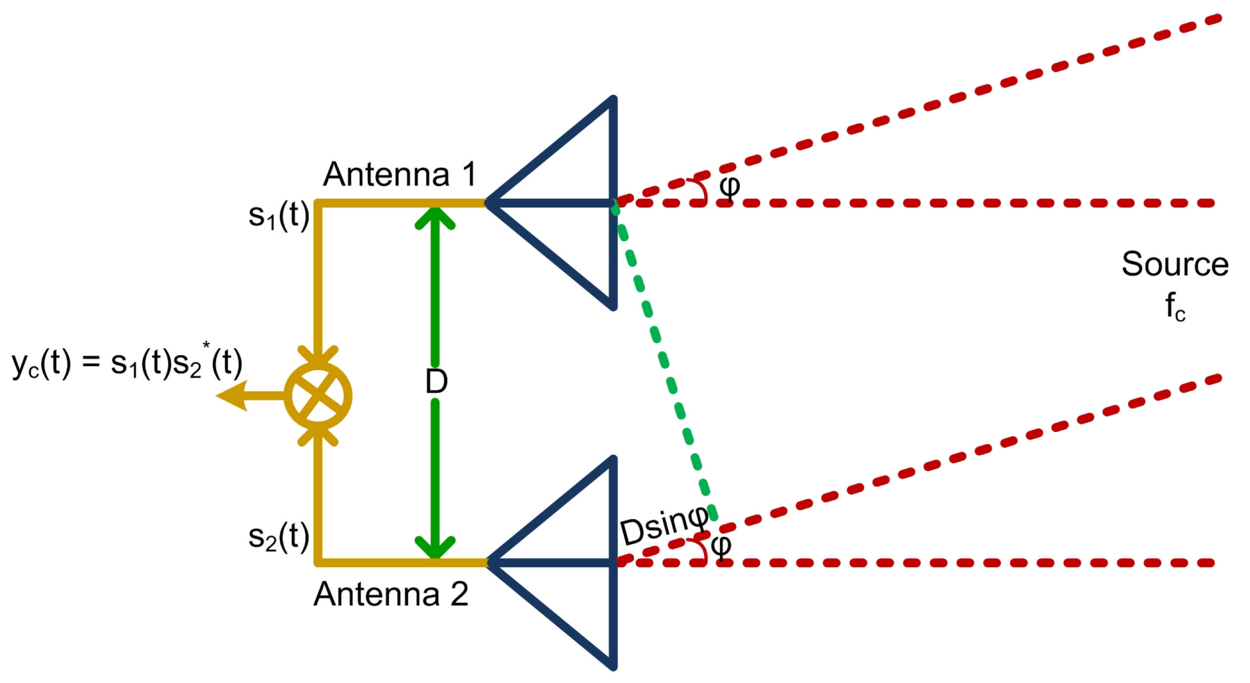
The interferometric radar is capable of measuring the angular velocity of moving object. It consists of two nominally identical receiving antennas separated by geometrical distance D as shown in Figure 2. The angular velocity of a point source moving across the interferometric beam causes fluctuation in the radar’s received signal.

The transmitted signal for FMCW radar with carrier frequency $f_c$, bandwidth B, and sweep duration T can be expressed as

$$S_T\left(t\right)=exp\{-j2\pi [f_c{t}_s+\frac{B}{2T}{t}_s^2]\}$$

(3)

where $t_s=t-nT$ is the time from the start of nth sweep. The signal reflected off of the target is same as the transmitted one, but delayed by a round trip time $\tau$. The signal received by the first antenna can be written as

$$S_{R_1}\left(t\right)=exp\{-j2\pi [f_c(t_s-\tau )+\frac{B}{2T}{(t_s-\tau )}^2]\}$$

(4)

where $\tau =2R/c=2(R_0+v_{r}nT)/c$, $R_0$ is the initial range of the target, and c represents the speed of light. The transmitted and received signals are mixed to generate beat frequency signal which is represented by

$$\begin{array}{cc}\hfill S_{B_1}\left(t\right)& =S_T\left(t\right)S_{R_1}^{*}\left(t\right)\hfill \\ \hfill & =exp\{-j4\pi [\frac{B(R_0+v_{r}nT)t_s}{cT}+\frac{R_0}{\lambda }+\frac{v_r}{\lambda }nT-\frac{B{(R_0+v_{r}nT)}^2}{c^{2}T}]\}\hfill \\ \hfill & \approx exp\{-j4\pi [\frac{B(R_0+v_{r}nT)t_s}{cT}+\frac{R_0}{\lambda }+\frac{v_r}{\lambda }nT]\}\hfill \end{array}$$

(5)

where $\lambda =c/f_0$ is the wavelength. The signal received by the second antenna $S_{R_2}\left(t\right)$, which is delayed by time ${\tau }_0$ due to the geometrical separation D between the two receiving antennas is expressed as

$$S_{R_2}\left(t\right)=exp\{-j2\pi [f_c(t_s-\tau -{\tau }_0)+\frac{B}{2T}{(t_s-\tau -{\tau }_0)}^2]\}$$

(6)

where time delay ${\tau }_0$ is denoted as

$${\tau }_0=\frac{D\sin \phi }{c}$$

(7)

Similarly, the second beat frequency signal is represented by

$$\begin{array}{cc}\hfill S_{B_2}\left(t\right)& =S_T\left(t\right)S_{R_2}^{*}\left(t\right)\hfill \\ \hfill & \approx exp\{-j2\pi [\frac{2B(R_0+V_{r}nT)t_s}{cT}+\frac{2v_{r}nT}{\lambda }+\frac{2R_0}{\lambda }+(f_c+\frac{B}{T}{t}_s)\frac{D\sin \phi }{c}]\}\hfill \end{array}$$

(8)

According to the interferometric radar principle, the two beat frequency signals $S_{B_1}\left(t\right)$ and $S_{B_2}\left(t\right)$ are correlated to generate the interferometric output,

$$\begin{array}{cc}\hfill y_c& =S_{B_1}\left(t\right)S_{B_2}^{*}\left(t\right)\hfill \\ \hfill & =exp\{j2\pi (f_c+\frac{B{t}_s}{T})\frac{D\sin \phi }{c}\}\hfill \end{array}$$

(9)

The time derivative of the phase term in Equation (9) provides the interferometric frequency shift caused by the angular velocity [26].

$$f_a=\frac{D\cos \phi }{{\lambda }_{t_s}}\omega \approx \frac{D}{{\lambda }_{t_s}}\omega$$

(10)

where ${\lambda }_{t_s}=c/(f_c+B{t}_s/T)$. By re-arranging Equation (10), the angular velocity can be expressed as

$$\omega =\frac{f_a{\lambda }_{t_s}}{D}$$

(11)

2.2. Process Model and Measurement Model

As mentioned earlier, MTT problem is to identify the number of potential targets in the radar’s FOV and estimate their kinematic states based on noisy radar measurements in the presence of clutter due to false alarm. Suppose that the target’s dynamic motion model can be represented by one of the r model hypotheses referred as $M_i:=\{1,2,\dots ,r\}$. $M_{k-1}^j$ denotes the event that dynamic model j was effective during the period $[t_{k-1},t_k]$. The jth hypothesis process model is represented as

$${\mathbf{x}}_k={\mathbf{F}}_{k-1}^j{\mathbf{x}}_{k-1}+{\mathbf{v}}_{k-1}^j$$

(12)

where ${\mathbf{F}}_{k-1}^j$ denotes the state transition matrix for model j at time instant $k-1$, ${\mathbf{x}}_k$ is the state of the target at instant k and ${\mathbf{v}}_{k-1}^j$ is independent and identically distributed (i.i.d) zero-mean Gaussian process noise with covariance ${\mathbf{Q}}_{k-1}^j$, i.e., ${\mathbf{v}}_{k-1}^j\sim \mathcal{N}(\mathbf{0},{\mathbf{Q}}_{k-1}^j)$.

Moreover, the state of target in terms of Cartesian coordinates at instant k is represented as

$${\mathbf{x}}_k={[x,v_x,y,v_y]}^T$$

(13)

where ($x,y$) and ($v_x,v_y$) are the Cartesian coordinates and velocities of the target, respectively, which satisfy $v_x=x^{{}^{\prime }}$ and $v_y=y^{{}^{\prime }}.$

The measurement model which establishes the relationship between the target state vector and radar measurements vector ${\mathbf{z}}_k$ is expressed as

$${\mathbf{z}}_k=\mathbf{h}\left({\mathbf{x}}_k\right)+{\mathbf{w}}_k$$

(14)

where $\mathbf{h}\left({\mathbf{x}}_k\right)$ is the nonlinear measurement function and ${\mathbf{w}}_k$ is assumed to be i.i.d. zero-mean Gaussian measurement noise with covariance ${\mathbf{R}}_k$, i.e., ${\mathbf{w}}_k\sim \mathcal{N}(\mathbf{0},{\mathbf{R}}_k)$ and $E\{{\mathbf{v}}_k{\mathbf{w}}_k^T\}=\mathbf{0}$. The measurement function is expressed as

$$\begin{array}{c}\hfill \mathbf{h}\left({\mathbf{x}}_k\right)=\left[\begin{array}{c}{v}_r\\ \omega \end{array}\right]\end{array}$$

(15)

Now, we derive the measurement function in terms of the dynamic state of the target. We know that $v_r=dR/dt$ and $\omega =d\phi /dt$. The relative range R of the target from radar and its DOA $\phi$ can be expressed as

$$R=\sqrt{{(x-x_s)}^2+{(y-y_s)}^2}$$

(16)

and

$$\phi ={tan}^{-1}\frac{(x-x_s)}{(y-y_s)}$$

(17)

where $(x_s,y_s)$ are coordinates of the radar location which is stationary. By taking the time derivative of Equation (16),

$$v_r=\frac{dR}{dt}=\frac{(x-x_s)v_x+(y-y_s)v_y}{\sqrt{{(x-x_s)}^2+{(y-y_s)}^2}}$$

(18)

Now by rearranging Equation (17) and then taking its time derivative,

$$tan\phi =\frac{(x-x_s)}{(y-y_s)}$$

(19)

$$\left({sec}^2\phi \right)\frac{d\phi }{dt}=\frac{(y-y_s)v_x-(x-x_s)v_y}{{(y-y_s)}^2}$$

(20)

$$\omega =\frac{d\phi }{dt}=[\frac{(y-y_s)v_x-(x-x_s)v_y}{{(y-y_s)}^2}]\left({cos}^2\phi \right)$$

(21)

$$\omega =[\frac{(y-y_s)v_x-(x-x_s)v_y}{{(y-y_s)}^2}][\frac{{(y-y_s)}^2}{R^2}]$$

(22)

$$\omega =\frac{(y-y_s)v_x-(x-x_s)v_y}{{(x-x_s)}^2+{(y-y_s)}^2}$$

(23)

According to Equations (18) and (23), the nonlinear measurement function $\mathbf{h}\left({\mathbf{x}}_k\right)$ can be expressed as

$$\begin{array}{c}\hfill \mathbf{h}\left({\mathbf{x}}_k\right)=\left[\begin{array}{c}{v}_r\\ \omega \end{array}\right]=\left[\begin{array}{c}\frac{(x-x_s)v_x+(y-y_s)v_y}{\sqrt{{(x-x_s)}^2+{(y-y_s)}^2}}\\ \\ \frac{(y-y_s)v_x-(x-x_s)v_y}{{(x-x_s)}^2+{(y-y_s)}^2}\end{array}\right]\end{array}$$

(24)

Based on this measurement function, our objective is to estimate the state ${\hat{\mathbf{x}}}_{k|k}=E\{{\mathbf{x}}_k|{\mathbf{z}}_k\}$ and error covariance ${\mathbf{P}}_{k|k}=E\{[{\mathbf{x}}_k-{\hat{\mathbf{x}}}_{k|k}]{[{\mathbf{x}}_k-{\hat{\mathbf{x}}}_{k|k}]}^T|{\mathbf{z}}_k\}$ for each target in the radar’s FOV. Moreover, the average number of clutter points assumes Poisson distribution and they are uniformly distributed in 2-D measurement space.

From Equation (23), it is clear that the angular velocity $\omega$ representing the angular rate of change is a relative measurement depending on the range of the target from the radar. It scales with the square of the relative range R. Therefore, the proposed MTT algorithm based on 2-D velocity measurements is applicable to short range surveillance applications for human targets and UAVs detection and tracking.

3. The Proposed Multi-Target Tracking Algorithm

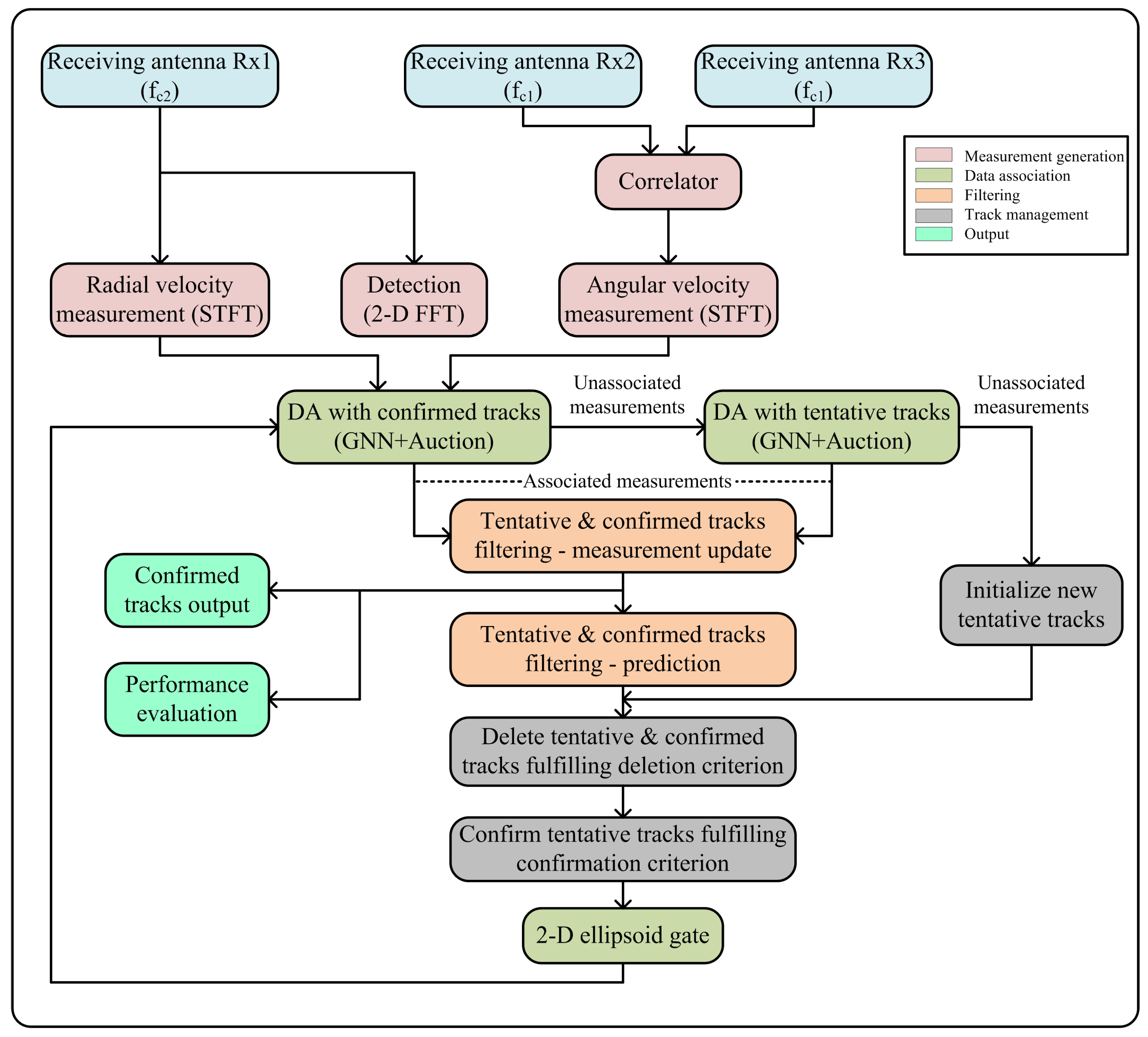
This section describes the design and implementation of the proposed MTT algorithm as delineated in Figure 3. The DF-FMCW radar is capable of operating in two different modes corresponding to $f_{c_1}$ = 6 GHz and $f_{c_2}$ = 24 GHz. It consists of two transmitting antennas (one operating at carrier frequency $f_{c_1}$ and second operating at carrier frequency $f_{c_2}$) [26]. There are three receiving antennas, Rx1 corresponding to $f_{c_2}$ and Rx2 and Rx3 corresponding to $f_{c_1}$ as shown in Figure 3.

• Detection and radial velocity measurement mode:
  For the purpose of detection and radial velocity measurement mode, the transmitting and receiving antennas operating at carrier frequency $f_{c_2}$ are connected to the processing unit. For detection, the radar scans the region of interest and range-radial velocity map is obtained by applying 2D fast Fourier transform (2D-FFT) to the beat frequency signal at the receiving antenna Rx1, providing the number of potential targets and their initial ranges. After detection, time-varying Doppler spectrogram is obtained by performing short-time Fourier transform (STFT) to the same beat frequency signal. According to Equation (1), the radial velocities of the targets are calculated by extracting their instantaneous frequencies from Doppler spectrogram.
• Angular velocity measurement mode:
  For angular velocity measurement, one transmitting and two receiving antennas operating at carrier frequency $f_{c_1}$ are connected to the processing unit. The two beat frequency signals at Rx2 and Rx3 are fed to the interferometric correlator to generate the output. Then, STFT is applied to the interferometric output to obtain the time-varying interferometric spectrogram. According to Equation (11), the angular velocities of targets are calculated by extracting their instantaneous frequencies from interferometric spectrogram.

Data association and state estimation by filtering are two major blocks of a multiple target tracking algorithm. Moreover, the two main data structures that include tentative and the confirmed tracks lists are handled by track management block. The track management block is responsible for new track initiation, tentative track confirmation (satisfying the confirmation criteria) and deletion of tentative and confirmed tracks (satisfying the deletion criteria). The confirmed tracks are less likely to be deleted as compared to the tentative tracks.

During each scan, when a new 2-D velocity measurement set from interferometric radar is received, it is first tested for association with the confirmed tracks. The data association for measurement-to-track pairing includes GNN method, which resolves the measurement conflict situations in terms of assignment problem. The auction method is the most efficient one to solve the assignment problems. The 2-D velocity measurements unassociated with confirmed tracks are then checked for association with the existing tentative tracks. The measurements that are still unassociated with any existing tracks are used for new track initiation.

The 2-D velocity measurements associated with the confirmed and tentative tracks are used for filter measurement update process. From Equation (24), it is clear that there is a nonlinear relationship between the kinematic state of the target and radar measurements. Therefore, a nonlinear filter algorithm is required for the target’s state prediction and measurement update steps. In the proposed tracking algorithm, IMM-SCKF estimator based on 2-D velocity measurement function is used for state estimation of different non-maneuvering and maneuvering target trajectories. The basic blocks of MTT algorithm are explained in detail in the subsequent sections of this paper for better understanding of the algorithm.

4. Data Association Using Global Nearest Neighbor (GNN) Method

Measurement-to-track association is a critical issue in case of multiple targets and cluttered environment. The main function of data association procedure is to determine the source of measurements received where multiple targets compete with each other for measurements or a single target validates multiple measurements. Allocating false measurements to the existing target tracks generally terminates these tracks.

Different techniques exist to solve the problem of data association which include nearest neighbor (NN), global nearest neighbor (GNN) [8,9], joint probabilistic data association (JPDA) [27,28,29,30], multiple hypothesis tracking (MHT) [31], and many more. The GNN algorithm makes hard assignment for measurement-to-track association, while the JPDA algorithm evaluates the probabilities of measurement-to-track association for multiple targets and combines them to obtain the state estimation. MHT is a powerful yet more complex method for MTT that evaluates the likelihood of a target existing given a train of measurements [8,9]. The authors of [32], evaluating the performance of different MTT algorithms for radar applications, assert the fact that GNN algorithm for data association outperforms other data association techniques in terms of tracking and robustness. GNN is the optimal data association technique for MTT which propagates single global hypothesis and resolves the measurement-to-track association in terms of optimal assignment problem [27,33].

Based on 2-D velocity measurement function represented by Equation (24), the data association procedure first forms an ellipsoid gate around the target’s predicted measurement, which is followed by GNN method to find the optimal assignment of measurements to tracks.

4.1. Ellipsoid Gating

Gating is a hard-decision technique to discard the unlikely measurement-to-track associations on the basis of dynamic motion model of the target [34]. All the measurements satisfying the gating relationship are considered to update the target track. The primary function of gating in data association is to reduce the computational complexity in advance [8,9].

For a measurement to fall within the ellipsoid gate of a track at instant k, the norm of the residual vector $d^2$ must satisfy the following criteria [8]:

$$d_k^2={\tilde{\mathbf{v}}}_k^T{\mathbf{S}}_{Z,k}^{-1}{\tilde{\mathbf{v}}}_k\le G$$

(25)

where ${\mathbf{S}}_{Z,k}$ is the measurement residual covariance matrix and G is the gate size. The measurement residual vector ${\tilde{\mathbf{v}}}_k$ based on 2-D velocity measurement function from Equation (24) is expressed as

$${\tilde{\mathbf{v}}}_k={\mathbf{z}}_k-\mathbf{h}\left({\hat{\mathbf{x}}}_{k|k-1}\right)$$

(26)

Generally, $d^2$ has chi-distribution (${\chi }_{n_z}^2$) for correct data association, where $n_z$ represents the dimension of measurement vector. The relationship between gate size G and probability of 2-D measurement vector to fall inside the gate $P_G\left(n_z\right)$ is expressed as [27]

$$P_G\left(2\right)=1-exp\left(\frac{-G}{2}\right)$$

(27)

4.2. Global Nearest Neighbor (GNN) Method

GNN is the most commonly used data association method which propagates a single global hypothesis by allocating the most eligible measurement to each track. It resolves the measurement conflict issue by forming and solving an assignment matrix. Input measurements occupy the rows of assignment matrix. The first columns of the assignment matrix are filled with the existing tracks, while the rest of the columns are occupied by new tracks, equal to the number of input measurements in the worst case scenario. The elements of assignment matrix are represented in terms of a score gain represented by:

$${\alpha }_{ij}=G-d_{ij}^2$$

(28)

Here, ${\alpha }_{ij}$ is the margin with which the normalized statistical distance $d_{ij}^2$ passed the gate for measurement i to track j association. The score gain for new track to a given measurement is set as zero. The forbidden assignments are represented by $-\infty$. The optimal assignment solution is the measurement set that not only maximizes the score gain, but maximizes the number of assignments as well [8,20].

Different methods exist to solve the problem of optimal assignment including Hungarian algorithm [35], Munkres algorithm [36], JVC algorithm [37], and Auction algorithm to list a few. Currently, the most efficient assignment algorithm is the auction algorithm which aims to maximize the score gain [8,9].

In the current work, based on 2-D velocity measurement function, we have implemented ellipsoid gating and GNN combined with auction method for data association. The difference from the existing work lies in the fact that conventional algorithms use either $(R,\phi )$ or $(R,v_r)$ measurements for all the steps of MTT algorithm. However, we have implemented the MTT algorithm based on 2-D velocity measurement for the target state estimation in terms of Cartesian coordinates and proved the effectiveness of the proposed algorithm for tracking.

Note that in conventional systems, the GNN method does not work well for closely spaced targets or crossing track patterns. However, in the proposed work based on 2-D velocity measurement function, it is not necessarily the case as closely spaced targets or crossing tracks may have different $(v_r,\omega )$ measurements even if they have same measurements in $(R,\phi )$ space. This fact has been verified in Section 8.5, simulation scenario 3 for crossing target tracks.

5. Target State Estimation Using IMM-SCKF Estimator

The primary objective of an estimation filter is to estimate the state of the detected target from noisy sensor measurements. The measurements associated to the targets during the data association procedure are used during the filter measurement update step.

According to Equation (24), as there is nonlinear relationship between 2-D velocity measurements and the state of the target, this work requires nonlinear estimation filter [27,33,38]. The Extended Kalman Filter (EKF) is the most common choice for nonlinear filtering problems [19]. However, for highly nonlinear systems, it tends to diverge quickly and has increased computational complexity [39]. The Unscented Kalman Filter (UKF) is capable of resolving these problems by using nonlinear unscented transform (UT). The UKF deterministically computes sigma points to calculate the mean and covariance of the propagated Gaussian distribution for nonlinear systems [40].

For nonlinear systems with additive Gaussian noise, the Cubature Kalman Filter (CKF) provides the closest approximation to Bayesian filtering [41]. The CKF is a cubature point filter which employs third-degree spherical-radial cubature rule for multidimensional integral approximation. It is numerically stable, computationally efficient and outperforms UKF for multidimensional nonlinear systems [42,43,44].

5.1. Square-Root Cubature Kalman Filter (SCKF)

In CKF, the matrix operations of inversion and square-root may cause the loss of symmetry and positive semi-definiteness properties of error covariance matrix leading to inaccurate results. The SCKF is numerically more stable and accurate than CKF as it propagates the square-roots of the error covariance matrix without the need of complex matrix operations [41,45]. One cycle of SCKF algorithm is presented below [46].

• Calculate the cubature points set ${\mathbf{X}}_i$ : (i = 1,2,…,m, where m = 2$n_x$)

  $${\mathbf{X}}_{i,k-1|k-1}={\mathbf{S}}_{k-1|k-1}{\xi }_i+{\hat{\mathbf{x}}}_{k-1|k-1}$$

  (29)

  $$\mathbf{P}=\mathbf{S}{\mathbf{S}}^T$$

  (30)

  $${\xi }_i=\sqrt{\frac{m}{2}}{[1]}_i$$

  (31)

  where $n_x$ is the dimension of state vector, ${\xi }_i$ represents weights of cubature points, and $\mathbf{S}$ represents square-root error covariance matrix.
• Time update: Propagate the cubature points and evaluate the predicted state and square-root error covariance.

  $${\mathbf{X}}_{i,k|k-1}^{*}=\mathbf{f}\left({\mathbf{X}}_{i,k-1|k-1}\right)$$

  (32)

  $${\hat{\mathbf{x}}}_{k|k-1}=\frac{1}{m}\sum _{m=1}^M{\mathbf{X}}_{i,k|k-1}^{*}$$

  (33)

  $${\mathbf{S}}_{k|k-1}=\mathbf{Tria}([{\mathcal{X}}_{k|k-1}^{*}{\mathbf{S}}_{Q,k-1}])$$

  (34)

  where

  $${\mathbf{Q}}_{k-1}={\mathbf{S}}_{Q,k-1}{\mathbf{S}}_{Q,k-1}^T$$

  (35)

  $$\begin{array}{c}\hfill {\mathcal{X}}_{k|k-1}^{*}=\frac{1}{\sqrt{m}}[{\mathbf{X}}_{1,k|k-1}^{*}-{\hat{\mathbf{x}}}_{k|k-1}{\mathbf{X}}_{2,k|k-1}^{*}-{\hat{\mathbf{x}}}_{k|k-1}\dots \\ \hfill {\mathbf{X}}_{m,k|k-1}^{*}-{\hat{\mathbf{x}}}_{k|k-1}]\end{array}$$

  (36)

  where $\mathbf{f}$(.) and ${\mathbf{S}}_Q$ represent nonlinear function of dynamic state equation and square-root process noise covariance matrix, respectively. Tria represents triangularization algorithm for matrix decomposition. Here, QR decomposition algorithm has been used.
• Measurement update: Calculate the propagated cubature points and update the state and square-root error covariance estimates.

  $${\mathbf{X}}_{i,k|k-1}={\mathbf{S}}_{k|k-1}{\xi }_i+{\hat{\mathbf{x}}}_{k|k-1}$$

  (37)

  $${\mathbf{Z}}_{i,k|k-1}^{*}=\mathbf{h}\left({\mathbf{X}}_{i,k|k-1}\right)$$

  (38)

  $${\hat{\mathbf{z}}}_{k|k-1}=\frac{1}{m}\sum _{m=1}^M{\mathbf{Z}}_{i,k|k-1}^{*}$$

  (39)

  $${\hat{\mathbf{x}}}_{k|k}={\hat{\mathbf{x}}}_{k|k-1}+{\mathbf{W}}_k({\mathbf{z}}_k-{\hat{\mathbf{z}}}_{k|k-1})$$

  (40)

  $${\mathbf{S}}_{k|k}=\mathbf{Tria}([{\mathcal{X}}_{k|k-1}-{\mathbf{W}}_k{\mathfrak{J}}_{k|k-1}{\mathbf{W}}_k{\mathbf{S}}_{R,k}])$$

  (41)

  where ${\mathbf{S}}_R$ represents square-root measurement noise covariance matrix. Square-root innovation covariance ${\mathbf{S}}_{zz,k|k-1}$, cros-covariance ${\mathbf{P}}_{xz,k|k-1}$, and square-root cubature Kalman gain ${\mathbf{W}}_k$ are represented by following equations.

  $${\mathbf{S}}_{zz,k|k-1}=\mathbf{Tria}([{\mathfrak{J}}_{k|k-1}{\mathbf{S}}_{R,k}])$$

  (42)

  $${\mathbf{R}}_k={\mathbf{S}}_{R,k}{\mathbf{S}}_{R,k}^T$$

  (43)

  $${\mathbf{P}}_{xz,k|k-1}={\mathcal{X}}_{k|k-1}{\mathfrak{J}}_{k|k-1}^T$$

  (44)

  $$\begin{array}{c}\hfill {\mathcal{X}}_{k|k-1}=\frac{1}{\sqrt{m}}[{\mathbf{X}}_{1,k|k-1}-{\hat{\mathbf{x}}}_{k|k-1}{\mathbf{X}}_{2,k|k-1}-{\hat{\mathbf{x}}}_{k|k-1}\dots \\ \hfill {\mathbf{X}}_{m,k|k-1}-{\hat{\mathbf{x}}}_{k|k-1}]\end{array}$$

  (45)

  $$\begin{array}{c}\hfill {\mathfrak{J}}_{k|k-1}=\frac{1}{\sqrt{m}}[{\mathbf{Z}}_{1,k|k-1}-{\hat{\mathbf{z}}}_{k|k-1}{\mathbf{Z}}_{2,k|k-1}-{\hat{\mathbf{x}}}_{k|k-1}\dots \\ \hfill {\mathbf{Z}}_{m,k|k-1}-{\hat{\mathbf{z}}}_{k|k-1}]\end{array}$$

  (46)

  $${\mathbf{W}}_k=({\mathbf{P}}_{xz,k|k-1}/{\mathbf{S}}_{zz,k|k-1}^T)/{\mathbf{S}}_{zz,k|k-1}$$

  (47)

5.2. Interactive Multiple Model (IMM) Estimator

As the moving target does not necessarily follow a single dynamic model, the modern tracking systems typically use IMM estimator for maneuvering targets tracking. The IMM estimator is capable of running multiple single model filters in parallel, with each filter following a different dynamic model with different process noise parameters [19,20]. The IMM-SCKF estimator has been used for maneuvering target tracking based on range-rate measurements from Doppler radar [45]. A single cycle of the IMM estimator is explained below [27].

• Mixing probabilities calculation:

  $${\overline{c}}^j=\sum _{i=1}^r{p}_{ij}{\mu }_{k-1|k-1}^i$$

  (48)

  $${\mu }_{k-1|k-1}^{(i,j)}=P\{M_{k-1}^i|M_k^j,{\mathbf{Z}}_1^{k-1}\}=\frac{1}{{\overline{c}}^j}{p}_{ij}{\mu }_{k|k-1}^i$$

  (49)

  where $\mu$ represents model probability and $p_{ij}$ are elements of model transition probabilities matrix. ${\mathbf{Z}}_1^{k-1}$ represents the measurement history from start to instant $k-1$.
• Interaction of state mean and covariance:

  $${\hat{\mathbf{x}}}_{k-1|k-1}^{0j}=\sum _{i=1}^r{\hat{\mathbf{x}}}_{k-1|k-1}^i{\mu }_{k-1|k-1}^{(i,j)}$$

  (50)

  $$\begin{array}{c}\hfill {\mathbf{P}}_{k-1|k-1}^{0j}=\sum _{i=1}^r{\mu }_{k-1|k-1}^{(i,j)}\{{\mathbf{S}}_{k-1|k-1}^i{({\mathbf{S}}_{k-1|k-1}^i)}^T+\\ \hfill [{\hat{\mathbf{x}}}_{k-1|k-1}^i-{\hat{\mathbf{x}}}_{k-1|k-1}^{0j}]{[{\hat{\mathbf{x}}}_{k-1|k-1}^i-{\hat{\mathbf{x}}}_{k-1|k-1}^{0j}]}^T\}\end{array}$$

  (51)
• State estimate update: The initial condition state estimate ${\hat{\mathbf{x}}}_{k-1|k-1}^{0j}$ and covariance matrix ${\mathbf{P}}_{k-1|k-1}^{0j}$ are fed to the SCKF algorithm described in previous section to compute the updated estimates ${\hat{\mathbf{x}}}_{k|k}^j$ and ${\mathbf{S}}_{k|k}^j$ for each filter model.
• Computing model likelihood function:

  $${\tilde{\mathbf{v}}}_k^j={\mathbf{z}}_k-\mathbf{h}({\hat{\mathbf{x}}}_{k|k-1}^j)$$

  (52)

  $${\mathbf{S}}_{Z,k}^j={\mathbf{A}}_k^j{({\mathbf{A}}_k^j)}^T$$

  (53)

  $${\wedge }_k^j=\frac{1}{\sqrt{|2\pi {\mathbf{S}}_{Z,k}^j|}}exp\{-0.5{[{\tilde{\mathbf{v}}}_k^j]}^T{[{\mathbf{S}}_{Z,k}^j]}^{-1}[{\tilde{\mathbf{v}}}_k^j]\}$$

  (54)
• Updating the model probability:

  $$c=\sum _{j=1}^r{\wedge }_k^j{\overline{c}}^j$$

  (55)

  $${\mu }_{k|k}^j=P\{M_k^j|{\mathbf{Z}}_1^k\}=\frac{1}{c}{\wedge }_k^j{\overline{c}}^j$$

  (56)
• Combining state mean and covariance estimates for output:

  $${\hat{\mathbf{x}}}_{k|k}=\sum _{j=1}^r{\hat{\mathbf{x}}}_{k|k}^j{\mu }_{k|k}^j$$

  (57)

  $${\mathbf{P}}_{k|k}=\sum _{j=1}^r{\mu }_{k|k}^j\{{\mathbf{S}}_{k|k}^j{({\mathbf{S}}_{k|k}^j)}^T+[{\hat{\mathbf{x}}}_{k|k}-{\hat{\mathbf{x}}}_{k|k}^j]{[{\hat{\mathbf{x}}}_{k|k}-{\hat{\mathbf{x}}}_{k|k}^j]}^T\}$$

  (58)

In the current work, IMM-SCKF based on the 2-D velocity measurement function has been used for filtering the targets present in confirmed track list. If a target in the track list does not receive any measurement, then the predicted state and error covariance matrix become the estimated state and error covariance matrix during the filtering process. Concerning the targets present in tentative track list, simple SCKF with nearly constant velocity (NCV) motion model is used. Depending on the clutter density, the number of tentative tracks is always greater than the number of confirmed tracks. Only a few of them qualify the criteria to be included in the confirmed track list. Therefore, using IMM-SCKF algorithm for the tentative tracks will result in computational load and increased complexity at the processing end.

6. Initial State Estimation

Initial state estimation is very crucial in target tracking applications, particularly in case of nonlinear process model or measurement model [19,20]. In the current work, as there is a nonlinear relation between the target state and measurements received, it is not possible to find analytical solution directly from the measurement model. However, according to the authors of [26], the initial measurements of range and azimuth angle (R,$\phi$) in the interferometric mode can be utilized to extract 2-D Cartesian initial position (x,y) of the target.

$$R_2-R_1=Dsin\phi$$

(59)

The target’s position estimates at two consecutive time steps are then used to estimate the target’s initial velocity from $v_x=(x_2-x_1)⁄T$ and $v_y=(y_2-y_1)⁄T$.

As the DOA $\phi$ is extracted from the range measurements, it is very sensitive to the error in range measurement. Therefore, we cannot rely on (R,$\phi$) measurements for the target tracking and state estimation. This information is used for initialization purpose only. Tracking is accomplished based on the 2-D velocity measurement.

7. Track Management Using Rule-Based M/N Logic

In MTT applications, the number of targets in the scan region does not remain constant. The function of the track management block is to handle the appearance and disappearance of these targets.

The GNN method, standalone, is not capable of handling track management. Therefore, we include rule-based M/N logic in track management step. The track management block represented by Figure 4 includes initiation of new tentative tracks, confirmation of tentative tracks, and deletion of tentative and confirm tracks when the targets no more exist. The output of data association block is fed to the track management unit to manage the tentative and confirmed track lists based on predefined rules. In both the tracks lists, each track consists of the following.

• State estimate ${\hat{\mathbf{x}}}_{k|k}$
• Square-root of error covariance estimate ${\mathbf{S}}_{k|k}$
• Residual covariance ${\mathbf{S}}_{Z,k}$
• Hit counter H
• Miss counter M

When a new set of 2-D velocity measurements arrives, these measurements are first examined for association with confirmed tracks. The measurements unassociated with confirmed tracks are then checked for association with tentative tracks. The unassociated measurements left after this step are used for new tentative track initialization and their ‘Hit’ and ‘Miss’ counters are set to 1 and 0, respectively. As a result of data association, if a tentative track gets associated with a measurement, its ‘Hit’ counter is increased, while ‘Miss’ counter remains unchanged. On the contrary, if a tentative track does not get associated with a measurement, its ‘Miss’ counter is increased, leaving ‘Hit’ counter unchanged.

In order for the tentative tracks to be inserted in the confirmed track list, it must fulfill 2/2 and 2/3 rule. If a tentative track receives measurements during first two consecutive scans, and then receives measurement at least twice during next three consecutive scans, then it fulfills the criteria to enter the confirmed track list. Otherwise, its delete flag is set to 1 and the tentative track will be deleted from the list. Once a tentative track enters the confirmed track list, its ‘Hit’ counter is set to 5 and ‘Miss’ counter is set to 0.

The deletion logic is less stringent when it comes to the confirmed tracks. If a confirmed track does not receive any measurement during data association, its ‘Hit’ counter is decreased and ‘Miss’ counter is increased. If the track does not receive measurements during five consecutive scans, i.e., Hit = 0 and Miss = 5, the delete flag for the confirmed track is set to 1 and the track is deleted from the confirmed track list.

8. Performance Evaluation Simulations

This section presents the performance evaluation of the proposed MTT algorithm on the basis of a set of performance evaluation metrics. Simulation results for different multiple targets scenarios (moving tangential to the radar broadside, crossing tracks and maneuvering targets) have been presented to verify the effectiveness of the proposed MTT algorithm.

8.1. Performance Evaluation Metrics

The performance evaluation metrics presented in this paper for the proposed MTT algorithm include the following.

• Root mean square error (RMSE) in position: Assume $[x_k,y_k]$ and $[{\hat{x}}_k,{\hat{y}}_k]$ represent the true and estimated positions, respectively, of a target at time instant k in $xy$-plane. The RMSE in position in terms of Cartesian coordinates at time instant k can be written as

  $${\mathrm{RMSE}}_k^{XY}=\sqrt{{({\hat{x}}_k-x_k)}^2+{({\hat{y}}_k-y_k)}^2}$$

  (60)
• Root mean square error (RMSE) in velocity: Similarly, if $[v_{x_k},v_{y_k}]$ and $[{\hat{v}}_{x_k},{\hat{v}}_{y_k}]$ represent the true and estimated velocities, respectively, of a target at time instant k, then the RMSE in velocity at time instant k can be written as

  $${\mathrm{RMSE}}_k^{v_x{v}_y}=\sqrt{{({\hat{v}}_{x_k}-v_{x_k})}^2+{({\hat{v}}_{y_k}-v_{y_k})}^2}$$

  (61)
• Posterior Cramer–Rao lower bound (PCRLB): PCRLB states that if both the state and measurement are random, then the state covariance matrix for an unbiased estimator is bounded as;

  $${\mathbf{P}}_{k|k}\ge {\mathbf{J}}_k^{-1}$$

  (62)

  where ${\mathbf{J}}_k$ represents Fisher information matrix (FIM) [47]. The PCRLB for the components of state vector can be calculated as

  $$\mathrm{PCRLB}\{[{\widehat{{\mathbf{x}}_k}]}_j\}={[{\mathbf{J}}_k^{-1}]}_{jj}$$

  (63)
• Mean execution time for one data scan ($T_E$): Mean execution time of algorithm for one cycle is computed by laptop computer. The specifications of computer are $1.9$ GHz processor, 4 GB RAM and Windows10 for Matlab2018. The total execution time is composed of time for data association ($T_{DA}$), target’s state estimation by filtering ($T_F$) and track management ($T_{TM}$) steps.
• IMM mean model probabilities: IMM mean model probabilities for maneuvering targets reflect how efficiently IMM algorithm can recognize different dynamic motion models of the targets and switch accordingly.

8.2. Parameter Selection and Simulated Data Generation

In order to evaluate the performance of the MTT algorithm, the targets are considered as point sources in far filed relative to the observing radar. A DF-FMCW interferometric radar with $f_{c_1}=6$ GHz and $f_{c_2}=24$ GHz is simulated with bandwidth $B=500$ MHz and sweep time $T_c=1$ ms. The sampling frequency is set to be $f_s=128$ kHz. The radar is placed at the origin of $xy$-plane and the two interferometric antennas corresponding to $f_{c_1}$ are located at (0,0) and (0,D), where $D=-3$.

To simulate the trajectories of the targets, two motion models have been considered.

Model 1: nearly constant velocity (NCV) motion model is used to simulate the uniform motion of the target. The NCV model for target state ${\mathbf{x}}_k={[x_x,v_{x_k},y_k,v_{y_k}]}^T$ along with discrete white noise acceleration (DWNA) model for process noise can be expressed as [27]

$${\mathbf{x}}_{k+1}={\mathbf{F}}_k^{\mathrm{NCV}}{\mathbf{x}}_k+{\mathsf{\Gamma }}_1{\mathbf{v}}_{1_k}$$

(64)

where

$$\begin{array}{c}\hfill {\mathbf{F}}_k^{\mathrm{NCV}}=\left[\begin{array}{cccc}1& T& 0& 0\\ 0& 1& 0& 0\\ 0& 0& 1& T\\ 0& 0& 0& 1\end{array}\right]\end{array}$$

(65)

and

$$\begin{array}{c}\hfill {\mathsf{\Gamma }}_1=\left[\begin{array}{cc}\frac{1}{2}{T}^2& 0\\ T& 0\\ 0& \frac{1}{2}{T}^2\\ 0& T\end{array}\right]\end{array}$$

(66)

T is sampling interval and ${\mathbf{v}}_{1_k}$ is zero-mean white Gaussian noise for small acceleration.

Model 2: nearly coordinated turn (NCT) motion model is used to simulate the circular or maneuvering segments of the target motion. The NCT model for target state ${\mathbf{x}}_k={[x_x,v_{x_k},y_k,v_{y_k},{\mathsf{\Omega }}_k]}^T$ along with DWNA model for process noise can be expressed as [27]

$${\mathbf{x}}_{k+1}={\mathbf{F}}_k^{\mathrm{NCT}}{\mathbf{x}}_k+{\mathsf{\Gamma }}_2{\mathbf{v}}_{2_k}$$

(67)

where

$$\begin{array}{c}\hfill {\mathbf{F}}_k^{\mathrm{NCT}}=\left[\begin{array}{ccccc}1& \frac{sin{\mathsf{\Omega }}_{k}T}{{\mathsf{\Omega }}_k}& 0& \frac{-(1-cos{\mathsf{\Omega }}_{k}T)}{{\mathsf{\Omega }}_k}& 0\\ \\ 0& cos{\mathsf{\Omega }}_{k}T& 0& -sin{\mathsf{\Omega }}_{k}T& 0\\ \\ 0& \frac{(1-cos{\mathsf{\Omega }}_{k}T)}{{\mathsf{\Omega }}_k}& 1& \frac{sin{\mathsf{\Omega }}_{k}T}{{\mathsf{\Omega }}_k}& 0\\ \\ 0& sin{\mathsf{\Omega }}_{k}T& 0& cos{\mathsf{\Omega }}_{k}T& 0\\ \\ 0& 0& 0& 0& 1\end{array}\right]\end{array}$$

(68)

and

$$\begin{array}{c}\hfill {\mathsf{\Gamma }}_2=\left[\begin{array}{ccc}\frac{1}{2}{T}^2& 0& 0\\ T& 0& 0\\ 0& \frac{1}{2}{T}^2& 0\\ 0& T& 0\\ 0& 0& T\end{array}\right]\end{array}$$

(69)

$\mathsf{\Omega }$ represents the turn rate and ${\mathbf{v}}_{2_k}$ is zero-mean white Gaussian process noise.

The standard deviations associated with linear and circular segments of target motion are assumed to be ${\sigma }_{v_1}=0.2$ and ${\sigma }_{v_2}=0.1$. Further, the radial velocity and angular velocity measurement error standard deviations are set as ${\sigma }_{v_r}=0.15 \mathrm{m} {\mathrm{s}}^{-1}$ and ${\sigma }_{\omega }=0.15 \mathrm{rad} {\mathrm{s}}^{-1}$, respectively. The probability of gate detection $P_G=0.99999$ which corresponds to gate size $G=23$.

The clutter points assume Poisson distribution and are uniformly distributed in the measurement region. Each clutter point is composed of (i) a radial velocity measurement distributed in the range of [$v_{{\mathrm{r}}_{\min }},v_{{\mathrm{r}}_{\max }}$] and (ii) an angular velocity measurement distributed in [${\omega }_{\min },{\omega }_{\max }$]. The average number of clutter points is set as 5 for each scan.

The model transition probabilities matrix for IMM filter is

$$\begin{array}{c}\hfill \pi =\left[\begin{array}{cc}0.99& 0.01\\ 0.01& 0.99\end{array}\right]\end{array}$$

(70)

The initial model probability for each filter model is chosen to be ${\mu }^j=0.5$, where $j=1,2$. The sampling interval is $T=0.02 \mathrm{s}$.

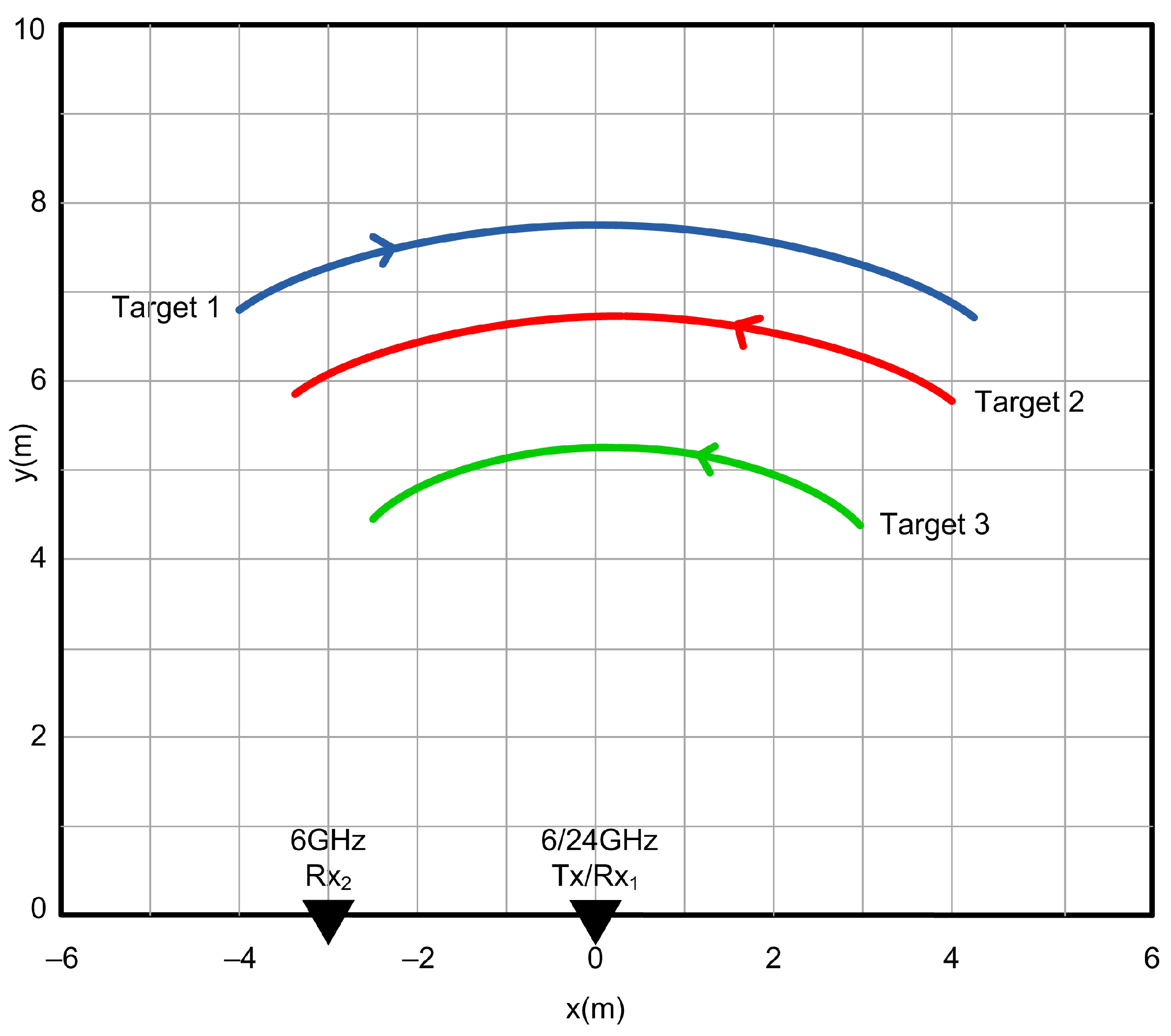
8.3. Scenario 1: Three Non-Maneuvering Targets Moving Tangential to the Radar Broadside

The radar and three non-maneuvering targets geometry for simulation scenario 1 is shown in Figure 5.

Table 1. Scenario 1.

Targets	Initial States of Targets
	x (m)	${\mathit{v}}_{\mathit{x}}$ (m s${}^{-1}$)	y (m)	${\mathit{v}}_{\mathit{y}}$$(\mathbf{m} \mathbf{s}{}^{\mathbf{-}\mathbf{1}})$	$\mathbf{\Omega }$ (rad s${}^{-1}$)
1	−4	7.9	6.6	4.8	−1.2
2	4	−6.6	5.5	4.8	1.2
3	3	−9.5	4.4	6.4	2.1

lists the initial states of the targets moving along the tangential to the radar following NCT motion model.

The range-radial velocity map ($f_{c_2}=24$ GHz) plotted in Figure 6a clearly shows three distinct targets with initial ranges of $R_{01}=7.7 \mathrm{m}$, $R_{02}=6.8 \mathrm{m}$, and $R_{03}=5.3 \mathrm{m}$, respectively. The initial radial velocities of the targets are $v_{r_1}=v_{r_2}=v_{r_3}=0 \mathrm{m} {\mathrm{s}}^{-1}$.

Time-varying Doppler spectrogram ($f_{c_2}=24$ GHz) and interferometric spectrogram ($f_{c_1}=6$ GHz) are presented in Figure 6b and Figure 6c, respectively. As the three targets are moving along the tangential to the radar broadside, the Doppler frequency shifts caused by the radial velocities are zero. Concerning the interferometric spectrogram, target 1 moving clockwise induces instantaneous interferometric frequency due to angular velocity in the positive zone, while target 2 and target 3 moving in counterclockwise direction induce instantaneous interferometric frequencies in the negative zone. Equations (1) and (11) are used to calculate the radial and angular velocities of the targets after extracting their instantaneous frequencies from the Doppler and interferometric spectrograms, respectively. Figure 6d,f represents the ideal and extracted radial and angular velocities of the targets, respectively.

Based on 2-D velocity measurements, the real and estimated target tracks are shown in Figure 6f. The real target tracks are plotted following NCT motion model from Equation (67), while the estimated tracks are the output of the proposed GNN-IMM-SCKF algorithm using 2-D velocity measurement function. To access the performance of the proposed algorithm, Figure 6g,h presents the RMSE in positions and velocities of three targets along with PCRLB. The large RMSE in the beginning is attributed to the state and error covariance matrix initialization. With the increasing number of measurement samples, the IMM-SCKF estimator converges and the RMSE decreases.

For simulation scenario 1, it is evident that the three targets moving tangential to the radar do not produce any Doppler frequency shift. Therefore, based on the Doppler frequency shift only, it is not possible to track these targets unless we have angular velocity information along with radial velocity measurement. The simulation results clearly demonstrate that the proposed MTT algorithm based on 2-D velocity measurements from interferometric radar is capable of tracking multiple targets moving with angular velocity only in 2-D Cartesian space which is not possible without Doppler radar network or phased array radar antennas.

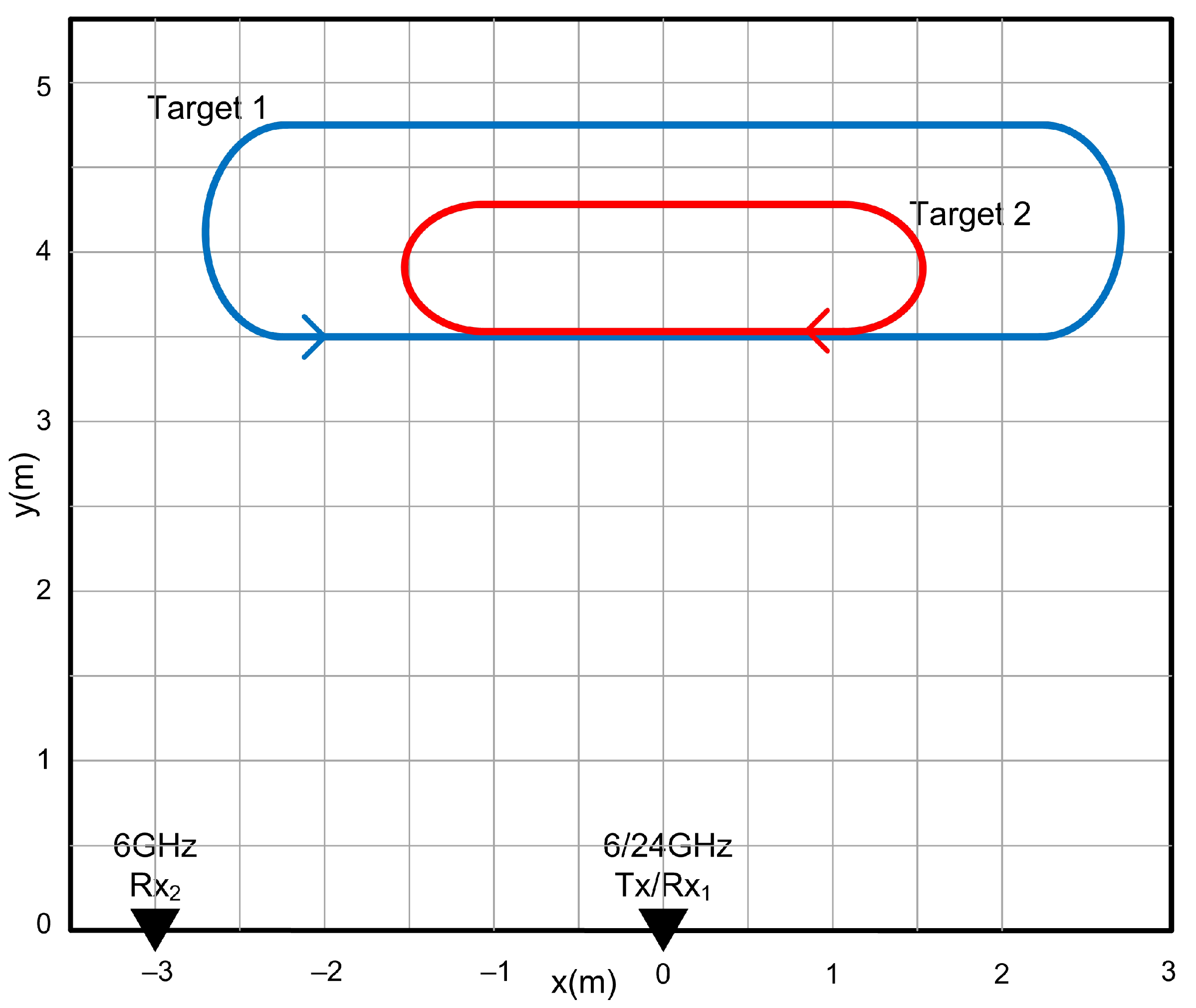
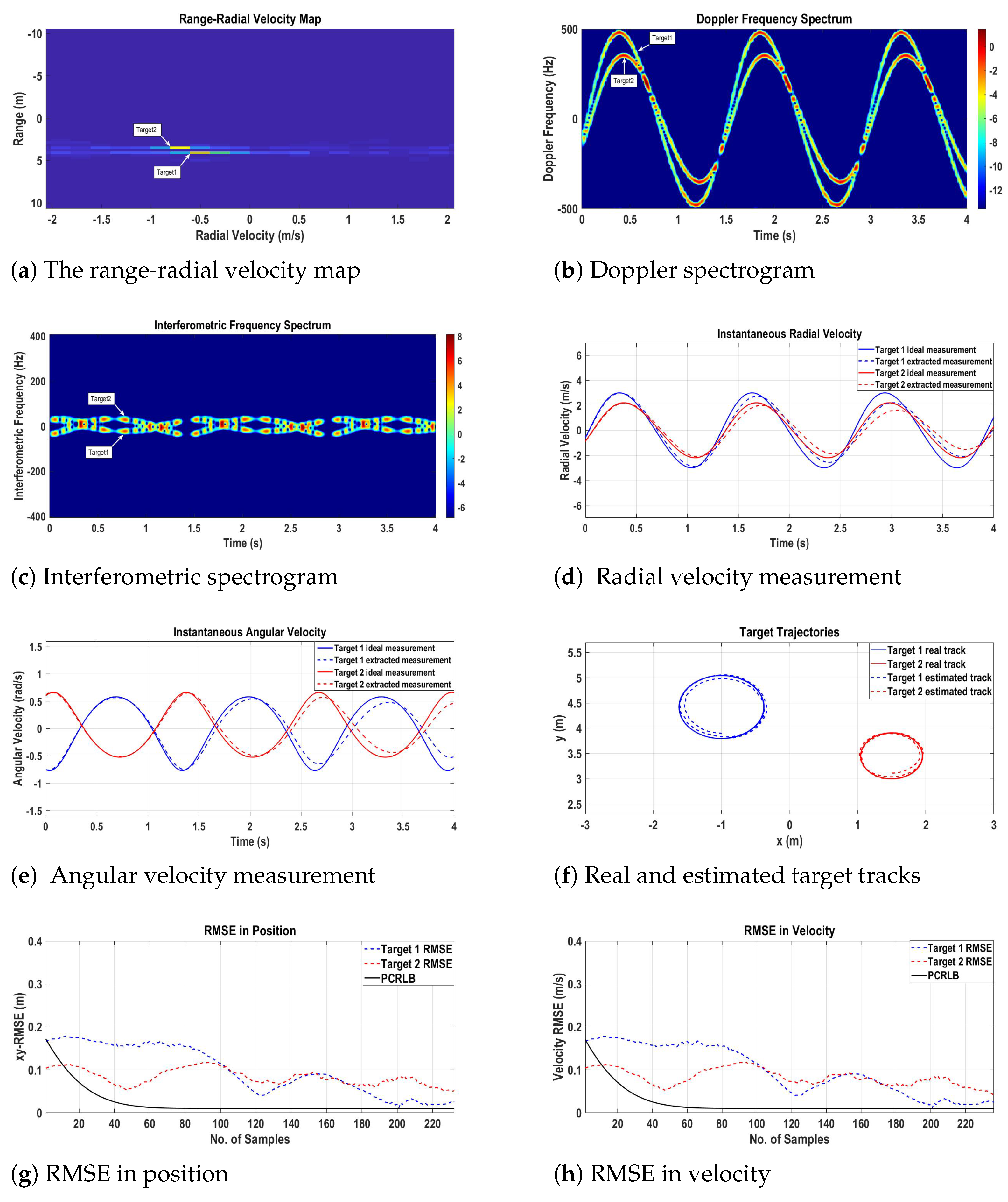
8.4. Scenario 2: Two Non-Maneuvering Targets with Circular Motion

The initial states of the targets for simulation scenario 2, presented by Figure 7, are summarized in

Table 2. Scenario 2.

Targets	Initial States of Targets
	x (m)	${\mathit{v}}_{\mathit{x}}$ (m s${}^{-1}$)	y (m)	${\mathit{v}}_{\mathit{y}}$$(\mathbf{m} \mathbf{s}{}^{-1})$	$\mathbf{\Omega }$ (rad s${}^{-1}$)
1	−1	3	3.8	0	4.8
2	1.5	−2.2	3	0	−4.8

. The two targets following NCT motion model are moving in circular path.

The range-radial velocity map for scenario 2 in Figure 8a depicts the presence of two targets with initial ranges of $R_{01}=4 \mathrm{m}$, $R_{02}=3.48 \mathrm{m}$ and initial radial velocities of $v_{r_1}=-0.5 \mathrm{m} {\mathrm{s}}^{-1}$ and $v_{r_2}=-0.7 \mathrm{m} {\mathrm{s}}^{-1}$.

Time-varying Doppler and interferometric spectrograms are shown in Figure 8b and Figure 8c, respectively. The sinusoidal patterns for both the Doppler and interferometric spectrograms caused by the radial and angular velocities of targets are in complete agreement with the circular motion of the targets in radar’s FOV.

The ideal and extracted radial and angular velocity measurements are plotted in Figure 8d and Figure 8e, respectively. The instantaneous radial and angular velocity extracted from time-varying Doppler and interferometric spectrograms are fed to the proposed MTT algorithm, which performs the data association, target state estimation and track management steps utilizing 2-D velocity measurement function. The real target tracks following Equation (67) and the output of the algorithm in the form of estimated target tracks in 2-D Cartesian space are shown in Figure 8f. The RMSE in positions and velocities of the targets shown in Figure 8g and Figure 8h, respectively, prove the validity of the proposed MTT algorithm for non-maneuvering target trajectories.

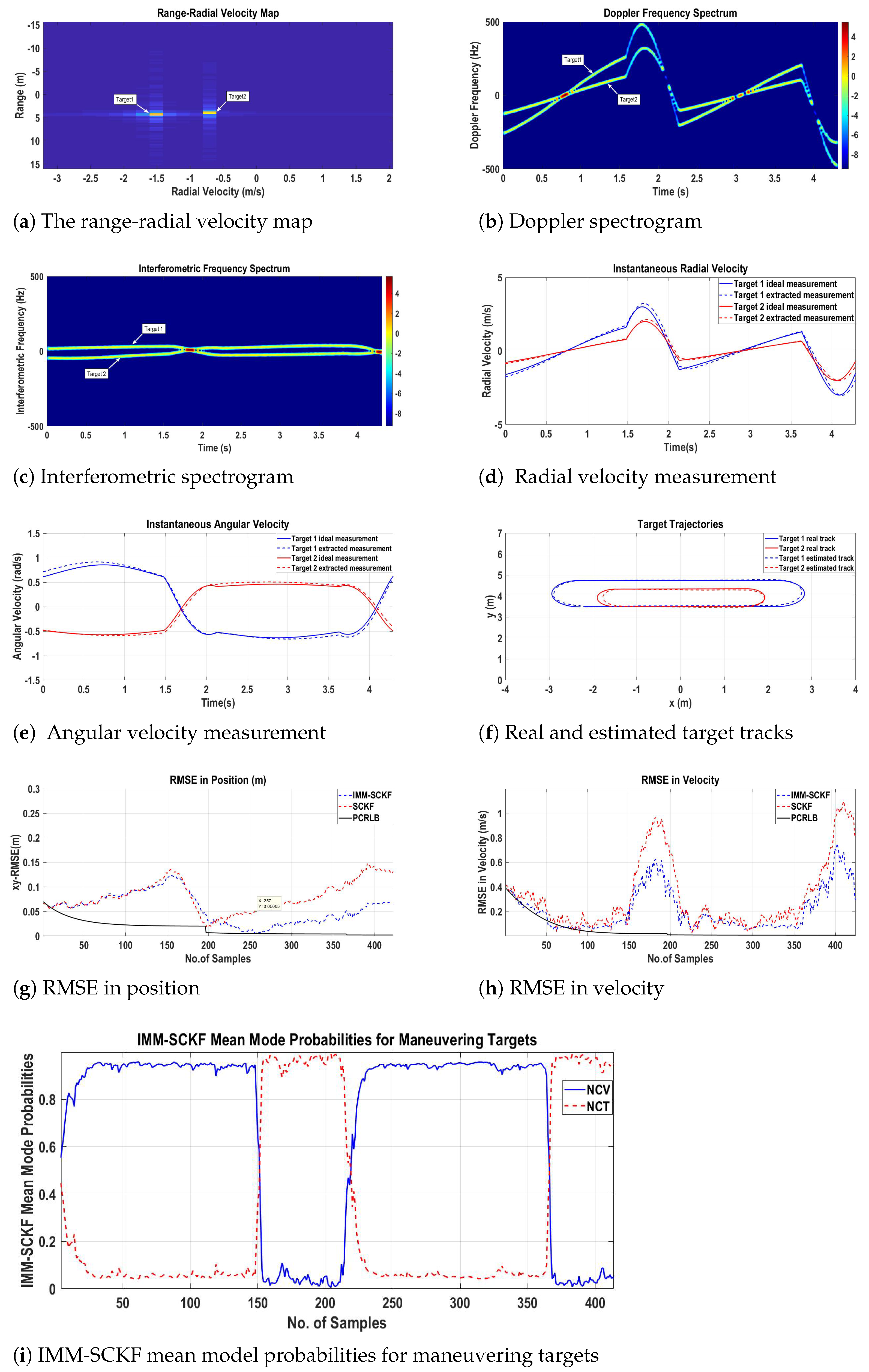
8.5. Scenario 3: Two Maneuvering Targets with Crossing Track Patterns

The geometry of radar and two maneuvering targets following NCV and NCT motion model is shown in Figure 9. The initial states of targets for simulation scenario are summarized in

Table 3. Scenario 3.

Targets	Initial States of Targets
	x (m)	${\mathit{v}}_{\mathit{x}}$ (m s${}^{-1}$)	y (m)	${\mathit{v}}_{\mathit{y}}$$(\mathbf{m} \mathbf{s}{}^{-1})$	$\mathbf{\Omega }$ (rad s${}^{-1}$)
1	−2.25	3	3.5	0	4.8
2	1.5	−2	3.5	0	−4.8

.

The range-radial velocity map for this scenario presented in Figure 10a shows two targets with initial ranges of $R_{01}=4.38 \mathrm{m}$, $R_{02}=4.08 \mathrm{m}$ and initial radial velocities of $v_{r_1}=-1.51 \mathrm{m} {\mathrm{s}}^{-1}$ and $v_{r_2}=-0.71 \mathrm{m} {\mathrm{s}}^{-1}$. Time-varying Doppler and interferometric spectrograms in Figure 10b,c are used to calculate the instantaneous radial and angular velocities of targets following Equations (1) and (11), respectively. Figure 10d,e represents the ideal and extracted radial and angular velocities of the targets, respectively.

The real tracks of two maneuvering targets following Equations (64) and (67) and the output of the proposed MTT algorithm presented in Figure 10f clearly show that the estimated target tracks follow the real target trajectories. Here, note that although the two targets are coming closer and cross each other near origin, GNN based on 2-D velocity measurement function is capable of performing correct data association which can be a problem with $(R,\phi )$ measurements.

To evaluate the performance of the proposed algorithm, RMSE in position and velocity of the targets have been plotted in Figure 10g,h. It can be clearly seen that the RMSE for GNN-IMM-SCKF algorithm is less as compared to the RMSE for the GNN-SCKF algorithm during maneuvering phases of the targets, which establishes the fact that the proposed algorithm with 2-D velocity measurements can be applied to IMM estimators for tracking. Figure 10i presents the IMM mean model probabilities for NCV and NCT models, where it is evident that IMM algorithm can efficiently distinguish and switch between different target motion models.

Finally,

Table 4. Execution times.

Scenario	Execution Time
	${\mathit{T}}_{\mathit{E}}$$(\mathbf{ms})$	${\mathit{T}}_{\mathbf{DA}}$ (ms)	${\mathit{T}}_{\mathit{F}}$ (ms)	${\mathit{T}}_{\mathbf{TM}}$ (ms)
1 (IMM-SCKF)	18.8	9.37 (50%)	6.02 (32%)	3.41 (18%)
2 (IMM-SCKF)	16.3	8.61 (53%)	4.56 (28%)	3.13 (19%)
3 (NCV-SCKF)	14.1	7.61 (54%)	3.52 (25%)	2.96 (21%)
4 (IMM-SCKF)	19.4	9.90 (51%)	6.50 (33%)	2.98 (16%)

reports the execution times for all the three simulation scenarios. It can be clearly seen that the data association time $T_{DA}$ dominates the execution times for filtering $T_F$ and track management $T_{TM}$ steps, which is approximately 50–54%. Furthermore, concerning scenario 3 total execution time for GNN-IMM-SCKF algorithm is increased as compared to GNN-SCKF algorithm. GNN-IMM-SCKF algorithm requires 38% more execution time than the time required for GNN-SCKF algorithm.

9. Conclusions

The paper presented multi-target tracking algorithm based on 2-D velocity measurements using dual-frequency FMCW interferometric radar, which removes the need of Doppler radar networks or expensive phased arrays to localize targets moving with small or no radial velocity in 2-D Cartesian space. First, we presented the mathematical model and implementation of the proposed MTT algorithm based on the derived 2-D velocity measurement function which established the relationship between the 2-D velocity measurements and state of the target in terms of Cartesian coordinates. Data association was performed using GNN method, and the states of the targets were estimated using IMM-SCKF estimator. The track management was accomplished using rule-based M/N logic. Second, the performance evaluation of the proposed algorithm was conducted for different scenarios with multiple targets including targets moving tangential to the radar broadside, crossing track patterns and maneuvering targets. In all scenarios, the performance was analyzed in terms of RMSE in position and velocity, PCRLB, execution time, and IMM mean model probabilities (for maneuvering targets) in the presence of process and measurement noise and cluttered environment. Simulation results established the fact that the proposed MTT algorithm based on the 2-D velocity measurement function using interferometric radar is robust, accurate, and can be implemented for practical real-time applications regardless of the target trajectories.