Classification of Targets Using Statistical Features from Range FFT of mmWave FMCW Radars

Abstract

Radars with mmWave frequency modulated continuous wave (FMCW) technology accurately estimate the range and velocity of targets in their field of view (FoV). The targeted angle of arrival (AoA) estimation can be improved by increasing receiving antennas or by using multiple-input multiple-output (MIMO). However, obtaining target features such as target type remains challenging. In this paper, we present a novel target classification method based on machine learning and features extracted from a range fast Fourier transform (FFT) profile by using mmWave FMCW radars operating in the frequency range of 77–81 GHz. The measurements are carried out in a variety of realistic situations, including pedestrian, automotive, and unmanned aerial vehicle (UAV) (also known as drone). Peak, width, area, variance, and range are collected from range FFT profile peaks and fed into a machine learning model. In order to evaluate the performance, various light weight classification machine learning models such as logistic regression, Naive Bayes, support vector machine (SVM), and lightweight gradient boosting machine (GBM) are used. We demonstrate our findings by using outdoor measurements and achieve a classification accuracy of 95.6% by using LightGBM. The proposed method will be extremely useful in a wide range of applications, including cost-effective and dependable ground station traffic management and control systems for autonomous operations, and advanced driver-assistance systems (ADAS). The presented classification technique extends the potential of mmWave FMCW radar beyond the detection of range, velocity, and AoA to classification. mmWave FMCW radars will be more robust in computer vision, visual perception, and fully autonomous ground control and traffic management cyber-physical systems as a result of the added new feature.

1. Introduction

There exists a wide variety of sensors for sensing and perception of the surrounding environment, such as camera, LiDAR, ultrasound, infrared (IR), thermal cameras, radar, accelerometers, gyroscopes, and global positioning system (GPS) to name a few. Although individual sensors are capable of extracting related features of the surrounding, they fail to obtain rich details necessary for reliable perception and navigation of autonomous systems [1,2,3,4]. When compared to ultrasound sensors that provide 1D information, vision-based sensors such as cameras provide more detailed 2D information, but they fail to perform under limited lighting conditions, such as during the night, and adverse weather such as rain and fog. Furthermore, spatio-temporal parameters of targets in the field of view can only be captured by lengthy computations, which can cause an unacceptable delay. Some of these problems, such as night vision or limited lighting conditions, can be solved to some extent by integrating IR cameras with cameras. Although machine learning techniques for training the model with images for object recognition and classification [5], as well as traffic sign recognition, are well developed, they are insufficient for fully autonomous and cyber-physical systems operating in varying weather conditions [6]. In addition, the camera fails to provide a 3D representation of the environment. In order to overcome these problems, LiDAR based sensing is one of the appealing approaches to acquiring a 3D map of the environment. However, there are still a number of challenges to overcome, such as reducing cost of the setup, reducing form factor, decreasing weight, and increasing number of channels for increased resolution while reducing latency when capturing the dynamics of objects in the FoV [1,2]. On the other hand, the mmWave radar sensors are single-chip radar sensors with extremely high resolution and low power consumption. These sensors work reliably in adverse weather conditions too, but no information on object morphology is obtained. The classification of different types of UAVs has been proposed by utilizing mmWave radars in [7]. Machine learning techniques are used to categorize activities using radar data. Drone type classification has been proposed in [8,9,10]. However, the proposed methods are computationally expensive. Recently, target classification using range-Doppler plots from a high density phase modulated continuous wave (PMCW) MIMO mmWave radar has been proposed in [11]. However, range-Doppler is a 2D FFT processing based approach that is also computationally complex. On the other hand, the target classification by mmWave FMCW radars using machine learning on range-angle images has been proposed in [12]. These range-angle images are created by utilizing range profiles obtained from a rotating radar. This approach is computationally less complex compared to previously mentioned approached but requires rotation. However, the various types of targets in classification under all weather conditions using low-complexity algorithms are still challenging.

In order o exploit the advantages of individual sensors, approaches based on sensor fusion has been implemented. For example authors in [13,14] fused data from camera and LiDAR to represent visual as well as depth information in a compact form and extracted the feature of the objects under interest. The disadvantages of this technique is that they require calibration and will result in enormous errors if not performed well. Similarly, radar-camera fusion for object detection, classification, and dynamics of environment is observed [15]. The drawback of the sensor fusion based technique is that they are flooded by a huge amount of data, e.g., image, video, and point cloud require additional computational cost.

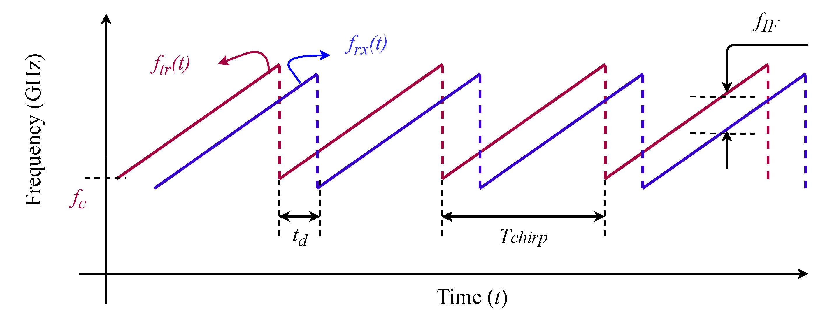
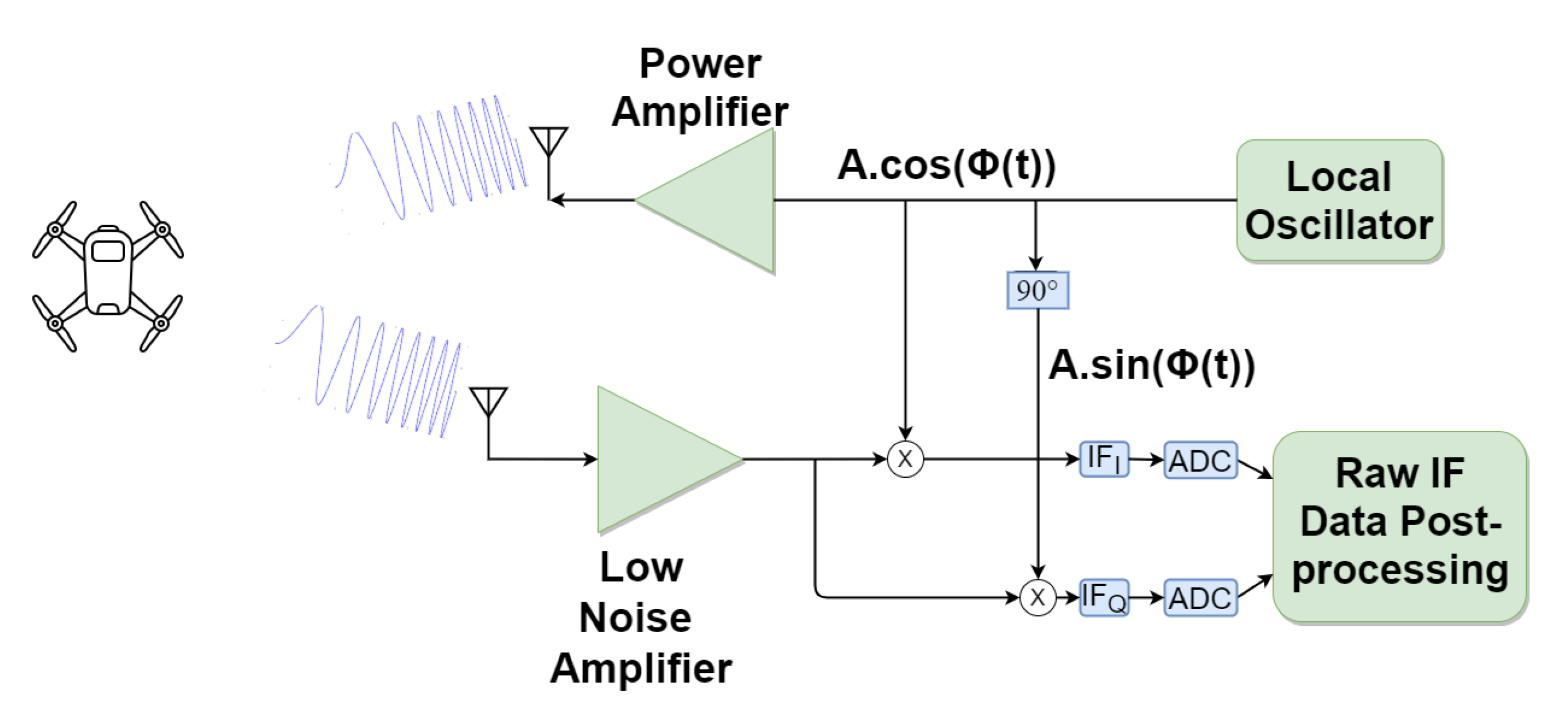
With the objective for detecting and classifying the objects with the limitations imposed by individual sensors, extensive signal processing of both the image and point cloud (2D or 3D data) radar, especially operating at the millimeter wave band, has been used recently for autonomous systems. Radars detect object parameters such as radial range, relative velocity, and the angle of arrival (AoA). While pulsed radar operate by finding the delay of the returned pulse from the remote object relative to the transmitted pulse, FMCW operates by transmitting frequency chirp and by beating the returned version with the transmitted ones, resulting in the intermediate frequency (IF), which contains information about the range and velocity of the objects. The FoV and/or beamwidth of mmWave FMCW radars are adjustable parameters up to 120° and maximum range of 300 m [16]. Furthermore, multiple radars can be cascaded together to achieve a wider FoV.

The fast Fourier transformation (FFT) on the IF signal provides range profile. The peaks in the range profile determines the radial range of the objects. In addition, time-frequency analysis techniques such as the Micro-Doppler have been investigated in some cases where targets have specific repeating patterns. This, however, increases the signal processing complexity, resulting in unacceptable latency in some application scenarios [17,18,19,20,21,22]. Furthermore, such techniques are limited to static targets [23,24]. Machine learning techniques have recently been investigated by using mmWave radars data. Surface classification with millimeter-Wave radar has been accomplished through the use of temporal features [25]. In [26], it was proposed to classify small UAVs and birds by using micro-Doppler signatures derived from radar measurements. The use of micro-Doppler spectrograms in cognitive radar for deep learning-based classification of mini-UAVs has been proposed in [27]. The cadence velocity diagram analysis has been proposed for detecting multiple micro-drones in [28]. Convolutional neural networks with merged Doppler images have been proposed in [8] for UAVs classification. The use of micro-Doppler analysis to classify UAVs in the Ka band has been proposed in [29]. The detection of small UAVs has been proposed using a radar-based EMD Algorithm and the extraction of micro-Doppler signals in [30]. The detection of small UAVs has been proposed using cyclostationary phase analysis on micro-Doppler parameters based on radar in [31]. UAV detection has been proposed by using regularized 2D complex-log spectral analysis and micro-Doppler signature subspace reliability analysis in [32]. A multilayer perceptron artificial neural network has been proposed for classifying single and multi-propelled miniature drones in [33]. It has been proposed to use FMCW radar to classify stationary and moving objects in road environments in [34]. The detection of road users such as pedestrians, cyclists, and cars using a 3D radar cube has been proposed by using CNN in [35]. CNN is used for classification, followed by clustering. Based on the Euclidean distance softmax layer, a method for classifying human activity by using mmWave FMCW radar has been proposed in [36]. Several deep learning-based methods for detecting human activity using radar are summarized in [37]. All of these works, however, used spectrograms or time-frequency representations derived from spectrograms, such as cepstrogram and CVD, which necessitates additional signal processing. The additional features of an intermediate frequency (IF) signal’s range FFT profile have not been thoroughly investigated. It has been demonstrated in [38] that by utilizing the features from the range FFT profile, additional information about the objects can be extracted.

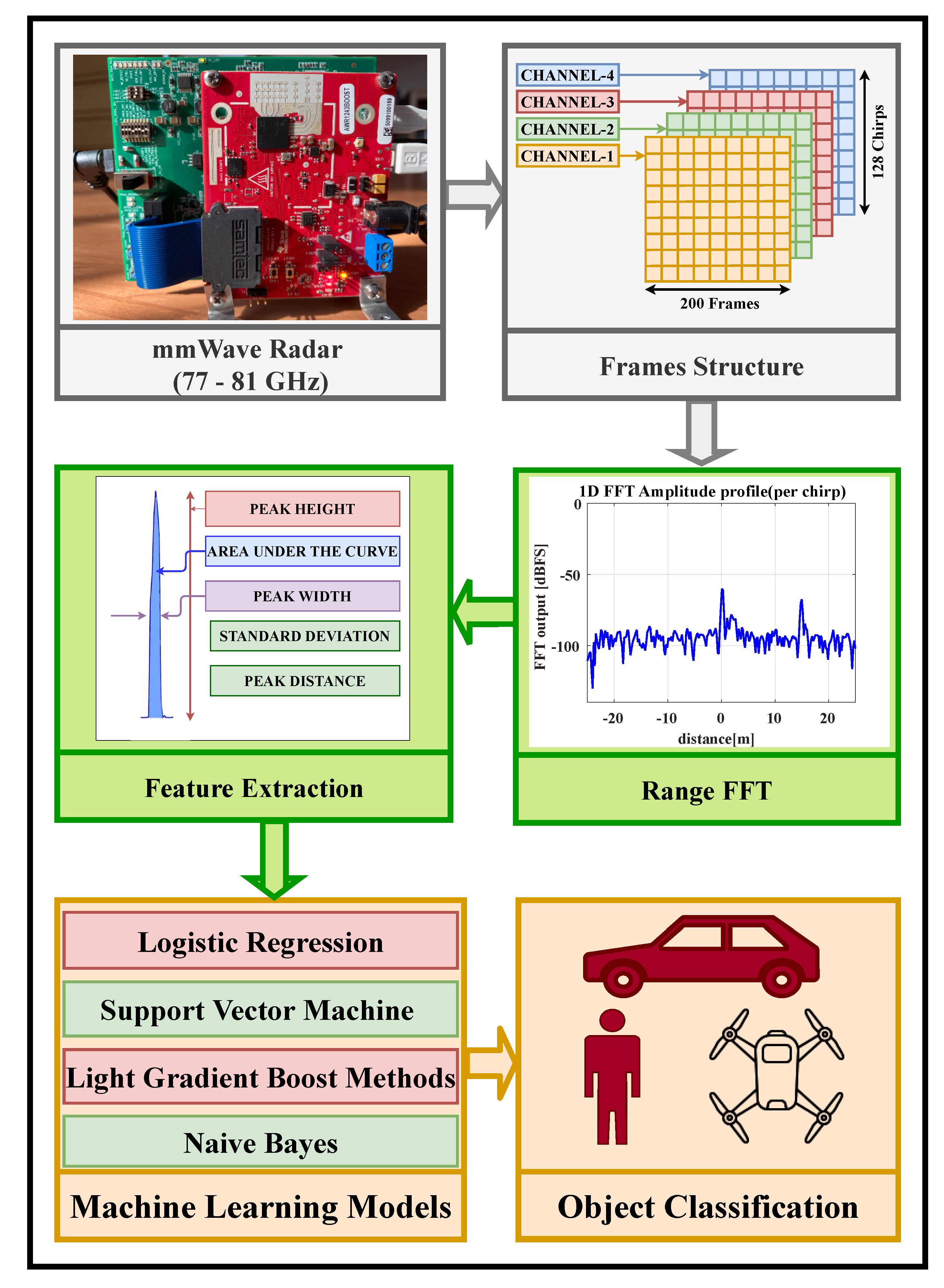
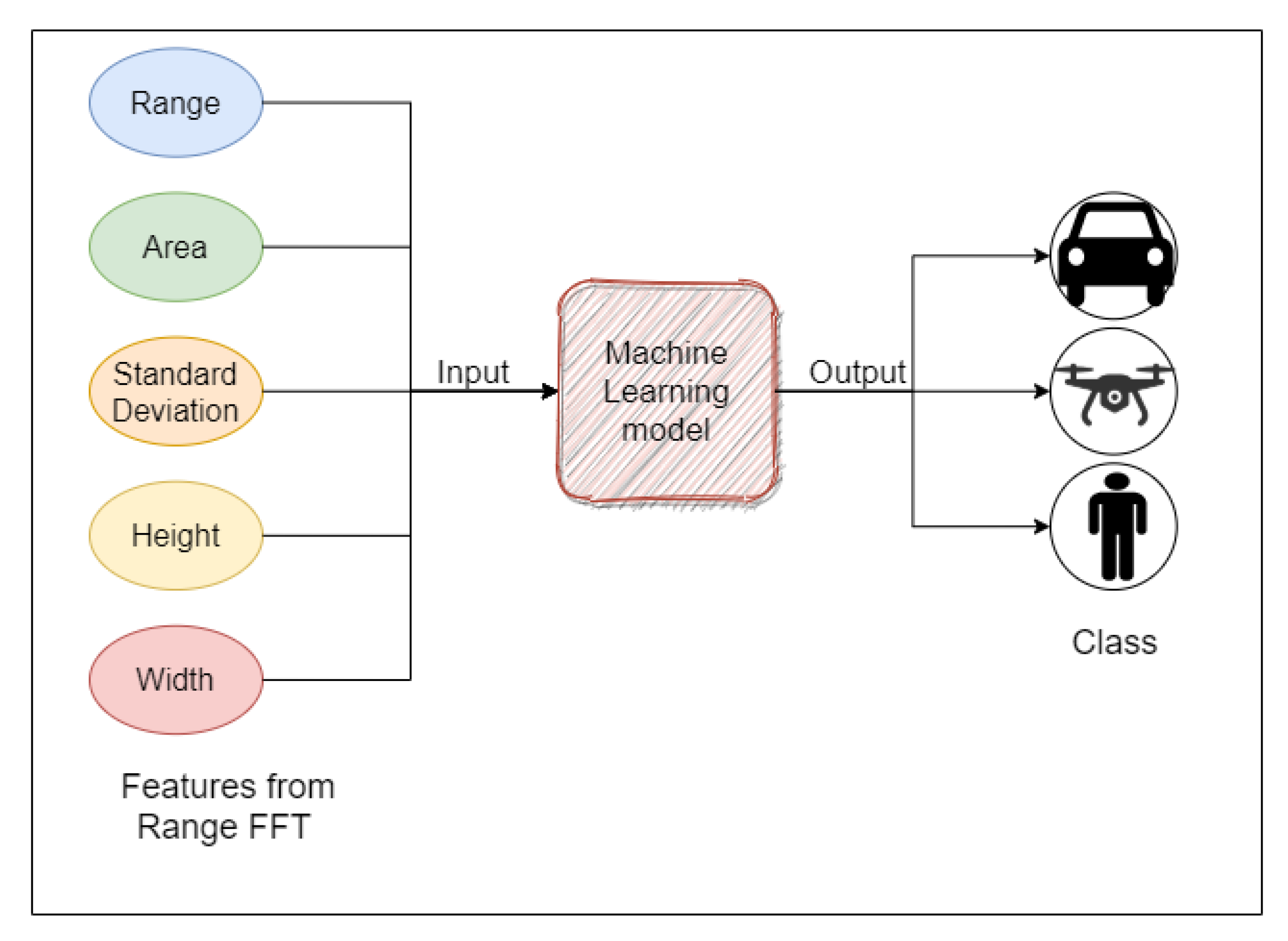
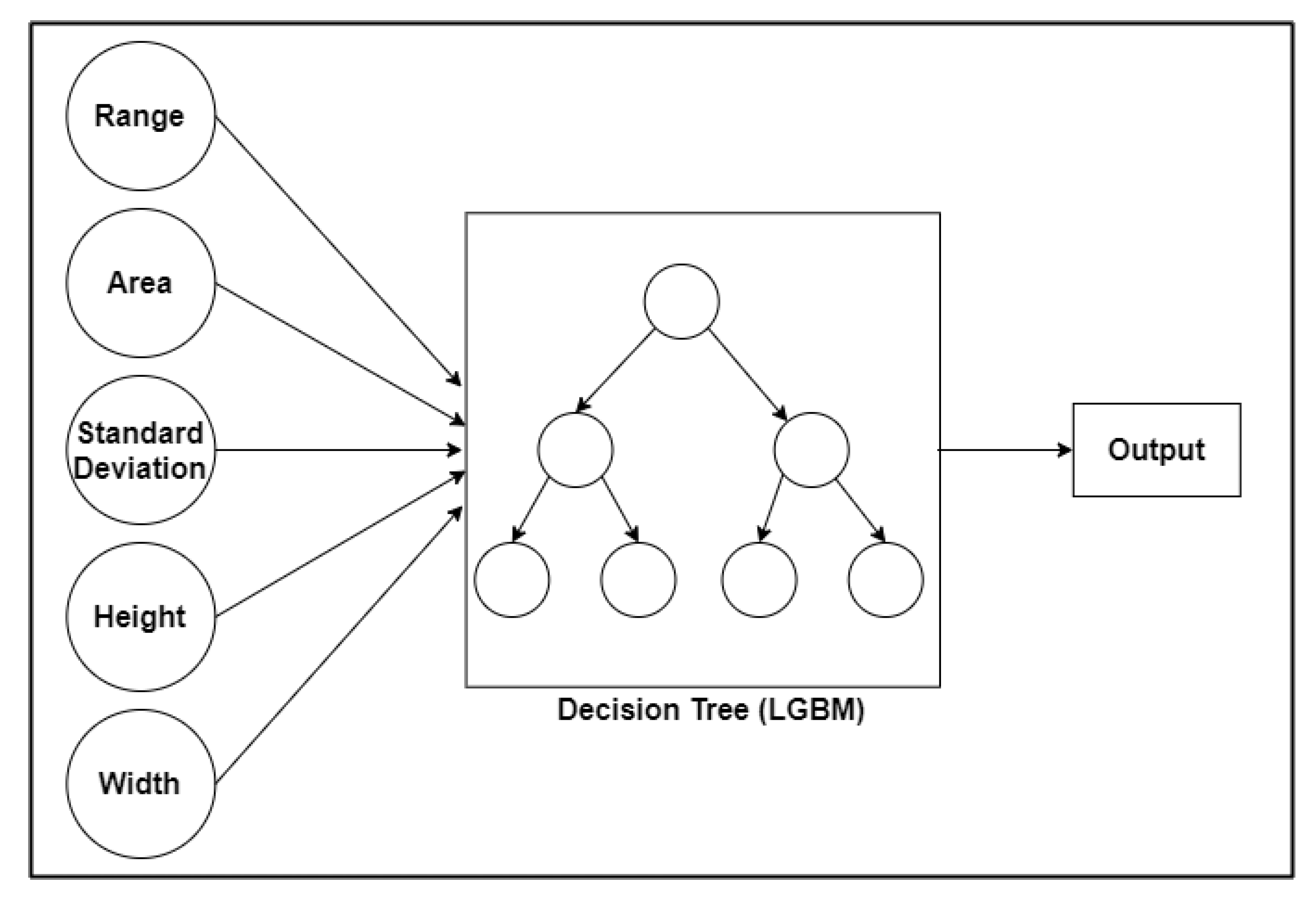
The ability to detect target features such as shape and size, as well as dynamic parameters of these targets, is critical. Such enhancements will improve the reliability and robustness of any system that utilizes radars. On the one hand, while the IF signal explicitly provides the object’s range, the distinguishing characteristics of the different objects are obtained by extracting statistical parameters from the range FFT plot, such as peak height, peak width, standard deviation, and area under peaks. Experiments have been carried out in order to categorize three common objects: an unmanned aerial vehicle (UAV), a car, and a pedestrian. A number of ML algorithms are used to classify the targets in combination with statistic features extracted from the IF signal range FFTs of the radar measures with different objects. Lightweight machine learning algorithms that have been investigated include Logistic Regression, Naive Bayes, support vector machine (SVM), and Light Gradient Boosted Machine (GBM). This is the first paper to use ML for classifying purposes with mmWave radars on the range FFT statistical features. The major contributions of the work are as follows:

• Outdoor experiments have been carried out to categorize three common objects: an unmanned aerial vehicle (UAV), a car, and a pedestrian.
• Extracting statistical parameters such as peak height, peak width, standard deviation, and area under peaks from the range profile of the radar data.
• Classification of the targets by using the statistical features extracted from the IF signal range FFTs of the radar measures with different objects and various ML models.

In complex situations, however, range profiles may not provide higher classification accuracy. The combination of mmWave radars with additional sensors such as RGB cameras, thermal cameras, and infrared cameras improves reliability and classification accuracy.

The rest of this paper is structured as follows. The system is described in Section 2. The experimental setup is described in detail in Section 3. Section 4 presents the data set, signal processing, details of the machine learning models, and the performances. The detailed data set and algorithms are available  at https://github.com/aveen-d/Radar_classification (accessed on 19 June 2021) [39].

Finally, the conclusion remarks together with possible future works are discussed in Section 5.

2. Measurement Setup and System Description

Figure 1 depicts the system-level diagram. There are six modules in total that are covered in detail in the sections below: (1) Data acquisition using mmWave FMCW radar; (2) Radar configuration details; (3) Range FFT/Range profile; (4) Features extraction using the identified peaks on Range FFT; (5) Target classification using Lightweight Machine learning models; and (6) Evaluation of performance of the classification models.

2.1. mmWave FMCW Radar and Data Acquisition

The measurements were taken outside by using a Texas Instruments complex base band FMCW mmWave radar (TI). The radar is equipped with four transmitting and three receiving antennas. The radar’s front-end complex base band architecture is depicted in Figure 2.

In Figure 3, the starting frequency ($f_c$), bandwidth (BW), and chirp slope (S) during one chirp period ($T_{chirp}$) are shown. The transmitted chirp’s instantaneous frequency is given by the following equation.

$$\begin{array}{cc}\hfill f_{tr}\left(t\right)& =f_c+S·t\hfill \\ \hfill & =f_c+\frac{BW}{T_{chirp}}t,0\le t\le T_{chirp}\hfill \end{array}$$

(1)

The transmitted chirp’s phase is given by the following equation.

$$\begin{array}{c}\hfill {\varphi }_{tr}\left(t\right)=2\pi f_{c}t+\pi \frac{BW}{T_{chirp}}{t}^2,\end{array}$$

(2)

Using (1) and (2), the transmitted chirp within a period ($T_{chirp}$) is given by the following equation:

$$\begin{array}{c}\hfill S_{tr}\left(t\right)=Acos(2\pi f_{tr}\left(t\right)t+{\varphi }_{tr}\left(t\right)),\end{array}$$

(3)

where $f_{tr}\left(t\right)$ represents the frequency of the transmitted chirp and ${\varphi }_{tr}\left(t\right)$ represents the phase of the transmitted chirp [40]. Similarly, the received signal following a remote target reflection is simply a delayed version of the transmitted signal and is given by the following:

$$\begin{array}{c}\hfill S_{rx}\left(t\right)=S_{tr}(t-\tau ),\end{array}$$

(4)

where $\tau =2R/c$ represents the time delay between the transmitted and received signal, R represents the radial range of the target from radar, and c represents the velocity of light in a vacuum.

The transmitting and receiving chirps patterns are depicted in Figure 3. The complex IF signal is created by combining the reflected chirp from the targets with the in-phase and quadrature-phase of the transmitted chirp, as illustrated in Figure 2. This complex IF signal is first processed with a low-pass filter before being digitized at a sampling rate of 10 Msps [2,40]. The frequency of IF signal is proportional to the radial range of the target and is given by (5).

$$\begin{array}{c}\hfill f_{IF}=\frac{BW·2R}{T_{chirp}·c},\end{array}$$

(5)

Range is given by (6):

$$R=\frac{f_{IF}c}{2S},$$

(6)

where $BW$, R, $f_{IF}$, c, and S represent the RF bandwidth, range, IF signal frequency, light velocity in vacuum, and chirp slope, respectively.

2.2. Radar Configuration Details

The mmWave radar configuration parameters are shown in

Table 1. Configuration parameters for the radar.

S. No.	Configuration Parameter	Value
1	Starting Frequency of the Chirp, fc	77 GHz
2	Bandwidth, BW	1798.92 MHz
3	Slope of the Chirp, S	29.982 MHz/µs
4	Number of Receiver Antennas	4
5	Number of Transmit Antennas	3
6	Number of ADC samples per chirp	256
7	Number of chirp loops	128
8	Number of frames	200
9	ADC Sampling rate	10 MSPS
10	Periodicity of the frame	40 ms
11	Rx Noise Figure	14 dB (76 to 77 GHz) 15 dB (77 to 81 GHz)
12	Transmission Power	12 dBm

. The raw ADC data of the complex IF signal are obtained from the radar and then post-processed in MATLAB in order to separate the data files for the four channels in the frame structure, as shown in Figure 4. Each measurement consists of 200 frames. Each frame is composed of 128 chirp loops, each of which contains 256 samples.

2.3. Range FFT

The FFT algorithm converts time-domain sampled complex IF signal data to frequency-domain. Each chirp/frame is processed to obtain the range FFT spectrum. After that, the range FFT is converted to an amplitude (dBFS) versus range (m) plot, where (6) can be used to calculate the range in meters from the frequency, and dBFS denotes the decibel full scale value of the signal amplitude. This range FFT plot is further processed by using peak detection algorithm. The peaks in the range FFT spectrum represent targets in the mmWave radar’s field of view.

The clutter is removed during preprocessing. Radar clutter is classified into two types: mainlobe clutter and sidelobe clutter [41]. The mainlobe clutter is caused by unwanted ground returns within the radar beamwidth (mainlobe), whereas the sidelobe clutter is caused by unwanted returns from any other direction outside the mainlobe. When the radar is placed at a lower height from the ground, the main lobe/sidelobe intersects the ground. Since the area of ground in the radar beam is often quite large, the ground return can be much larger than the target return. The clutter associated with ground returns close to the radar is removed by removing the associated components per range bin in range FFT.

2.4. Features Extraction

Feature extraction details are presented in this section. The range FFT plot is used to identify peaks, and then features for each peak are extracted. Among the features derived from the detected peaks in the FFT spectrum are the radial range of the target, the height of the peak, the peak width, the standard deviation, and the area under the peak. In general, only peaks are used to determine whether or not a target is present in the radar’s field of view [42,43,44,45]. Although other target parameters such as velocity and angle of arrival can be extracted from the radar measurements, target features such as size and shape cannot be estimated. However, targets can be classified by combining the aforementioned range FFT features with lightweight machine learning models.

2.5. Machine Learning Models

Once features are extracted, light weight machine learning techniques such as Logistic Regression, Support Vector Machine, Light Gradient Boost methods, and Naive Bayes are used. These machine learning models, as well as their key performance outcomes, are elaborated in detail in Section 4.

2.6. Target Classification

Three common targets such as a car, a pedestrian, and a UAV, are classified by using the extracted range profile features and lightweight machine learning models. By taking measurements with the targets of interest, additional targets can be added to the model.

3. Measurements and Signal Processing

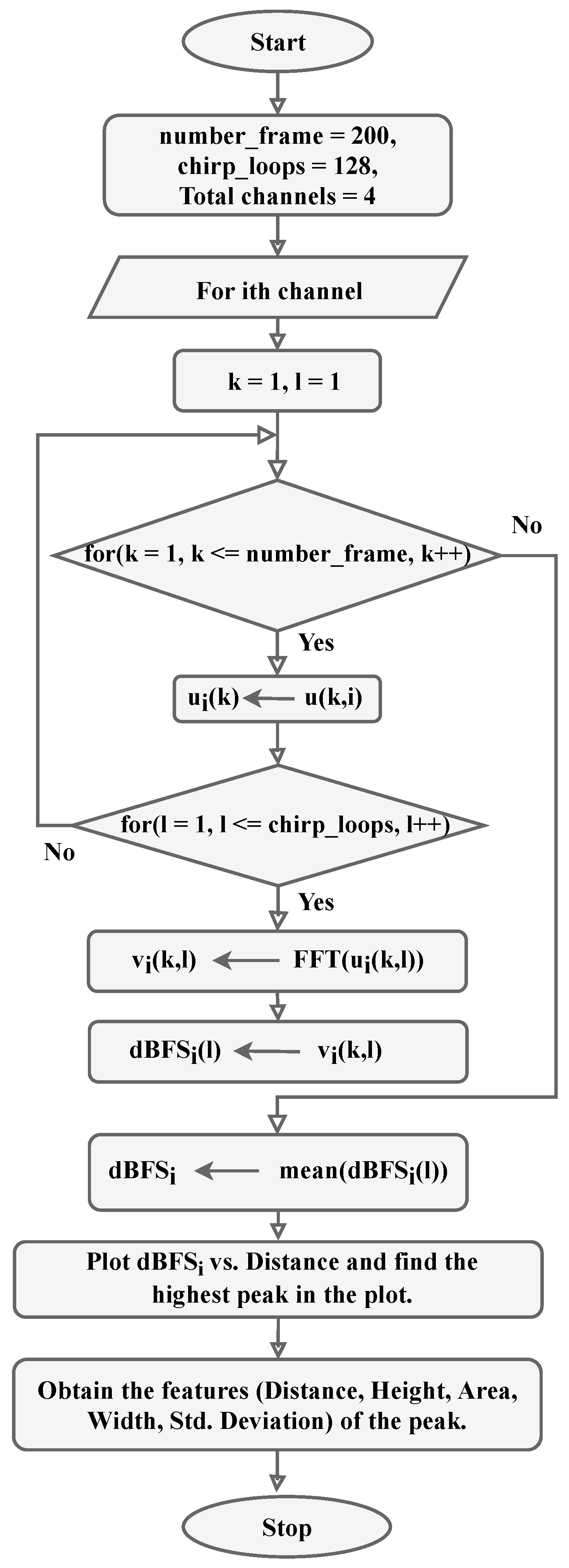
The measurement setup is lightweight and portable. It is made up of a mmWave FMCW radar with three transmitters and four receivers that operate in the frequency range of 77 to 81 GHz. The Texas Instruments’ mmWave Studio application is used to configure and control the radar setup. The configuration parameters of the radar used in these measurements are shown in Table 1. The algorithm used for the feature extraction of the objects is shown in Algorithm 1. 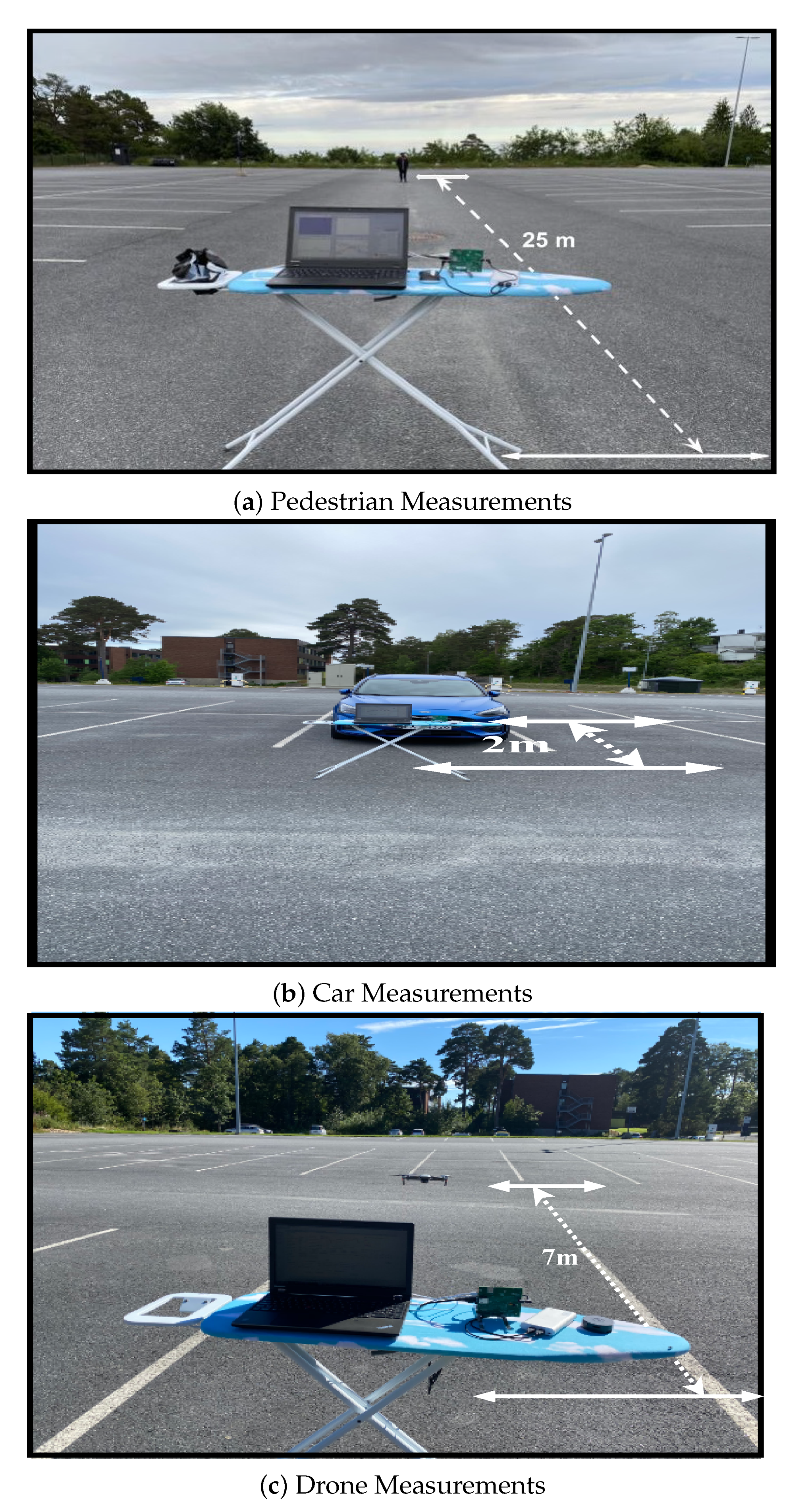A flowchart is shown in Figure 5 to explain the algorithm. 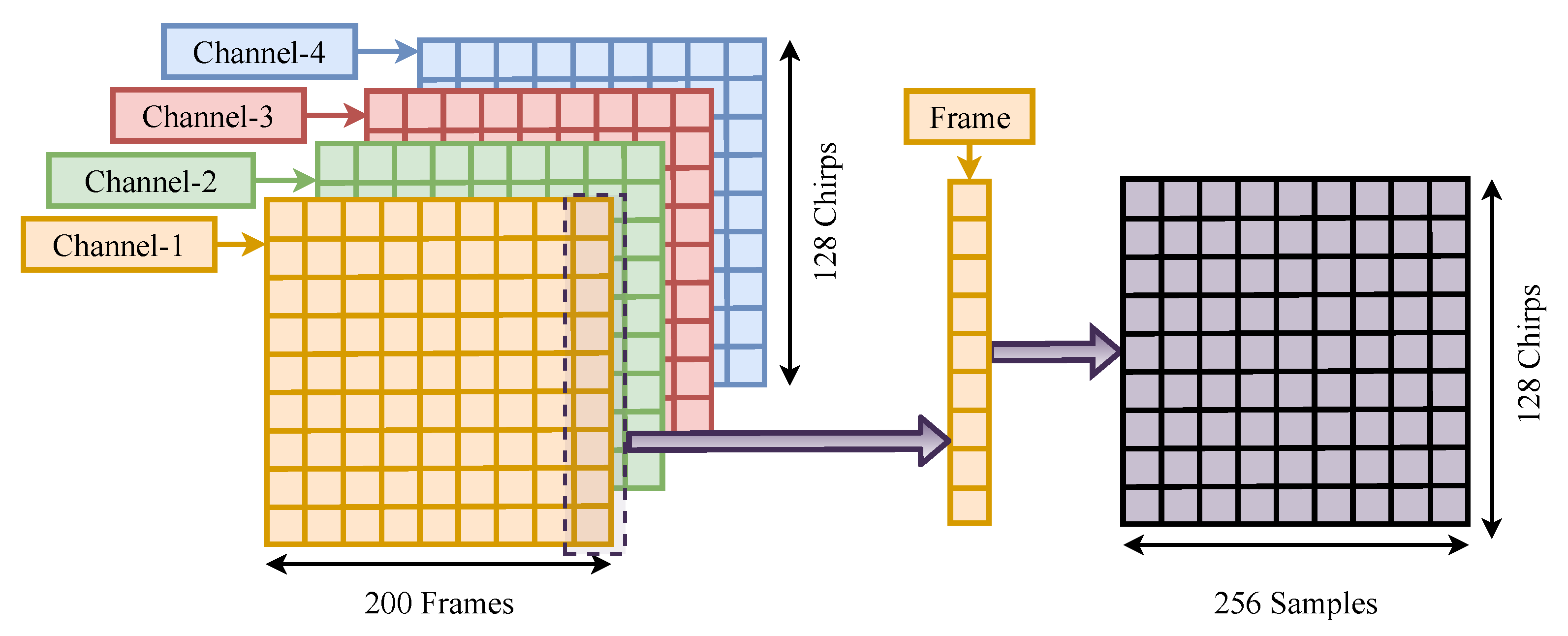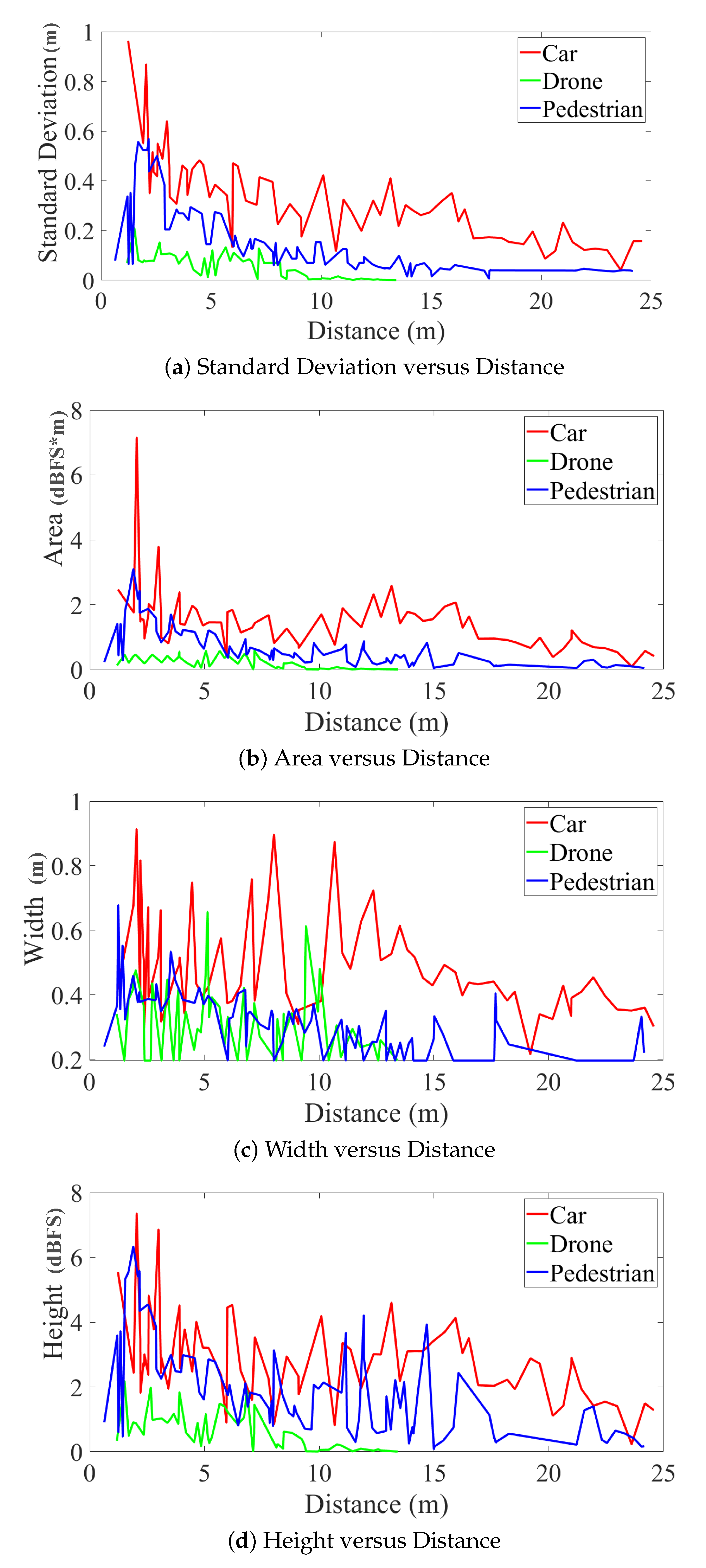Measurements are made with three common objects in an outdoor environment, as shown in Figure 6. Drone used in the measurements is quite small in size, and it possesses a size of 214 × 91 × 84 mm when folded and 322 × 242 × 84 mm when unfolded. The vehicle used was a medium-sized automobile with dimensions of 4315 × 1780 × 1605 mm. Measurements for the pedestrian were taken with a 172 cm tall adult. All three objects are one of a kind, with distinct shapes and sizes. For each object, several measurements were taken in small range steps up to a range of 25 m, which was the measurement scene’s limitation. The radar station is fixed and objects were moved from the radar in small steps while taking the measurements. The data collected using mmWave sensor are arranged for four channels, and post processing is performed on 200*128 chirp loops of a channel. A Fast Fourier Transform is applied on these chirp loops consisting of 256 samples/chirp loop. Further dBFS and a mean of dBFS of all these chirploops is calculated for 256 samples. The mean dBFS vs. distance plot is obtained using MATLAB. The highest peak in the plot will indicate the object location. A sharp peak can be obtained after the removal of a static plane. The features of the highest peak are extracted from this plot. This work has established a relationship between these extracted peak features and the object. This relationship is used to identify the type of object present in the vicinity of the mmWave sensors. All the extracted features from the measurements are shown in Figure 7. It is clear from Figure 7 that features extracted from the range FFT plot, such as standard deviation of the peak, area under the peak, the peak width, and the peak height, provide distinguishable information about the targets. This makes sense because targets with a large cross-section reflect more power and, as a result, larger peaks in the range FFT plot.

Algorithm 1 Object detection and features extraction from range FFT of mmWave FMCW radar.

Require:  $Object\_features$ from raw IF signal data u having $number\_frame$ = 200, $chirp\_loops$ = 128; for$k\leftarrow 1$ to $number\_frame$ do Ensure:    Raw IF signal ADC data u contains complex data of the IF signal i.e., raw IF signal ADC data corresponding to receiver i = 1, 2, 3, 4, for $max\_frame$ = 200, $chirp\_loops$ = 128 of raw data u. $u_i\left(k\right)\leftarrow u(k,i)$ for$l\leftarrow 1$ to $chirp\_loops$ do Ensure:    FFT with Hanning window of raw IF signal data u for receiver i = 1, 2, 3, 4 of $kth$ frame, $lth$ chirp. $v_i(k,l)\leftarrow FFT\left(u_i(k,l)\right)$   dBFS values are calculated for each chirp FFT. $\left[dBF{S}_i\left(l\right)\right]\leftarrow v_i(k,l)$   end for  end for Ensure:  Mean dBFS is calculated for all frames and chirps. $dBF{S}_i\leftarrow mean\left(dBF{S}_i\left(l\right)\right)$ Ensure:  Distance, height, width, and standard deviation of the peaks are calculated for the target detected using findpeaksSb function. $features(dis,ht,wd,ar,std)\leftarrow findpeaksSb\left(dBF{S}_i\right)$

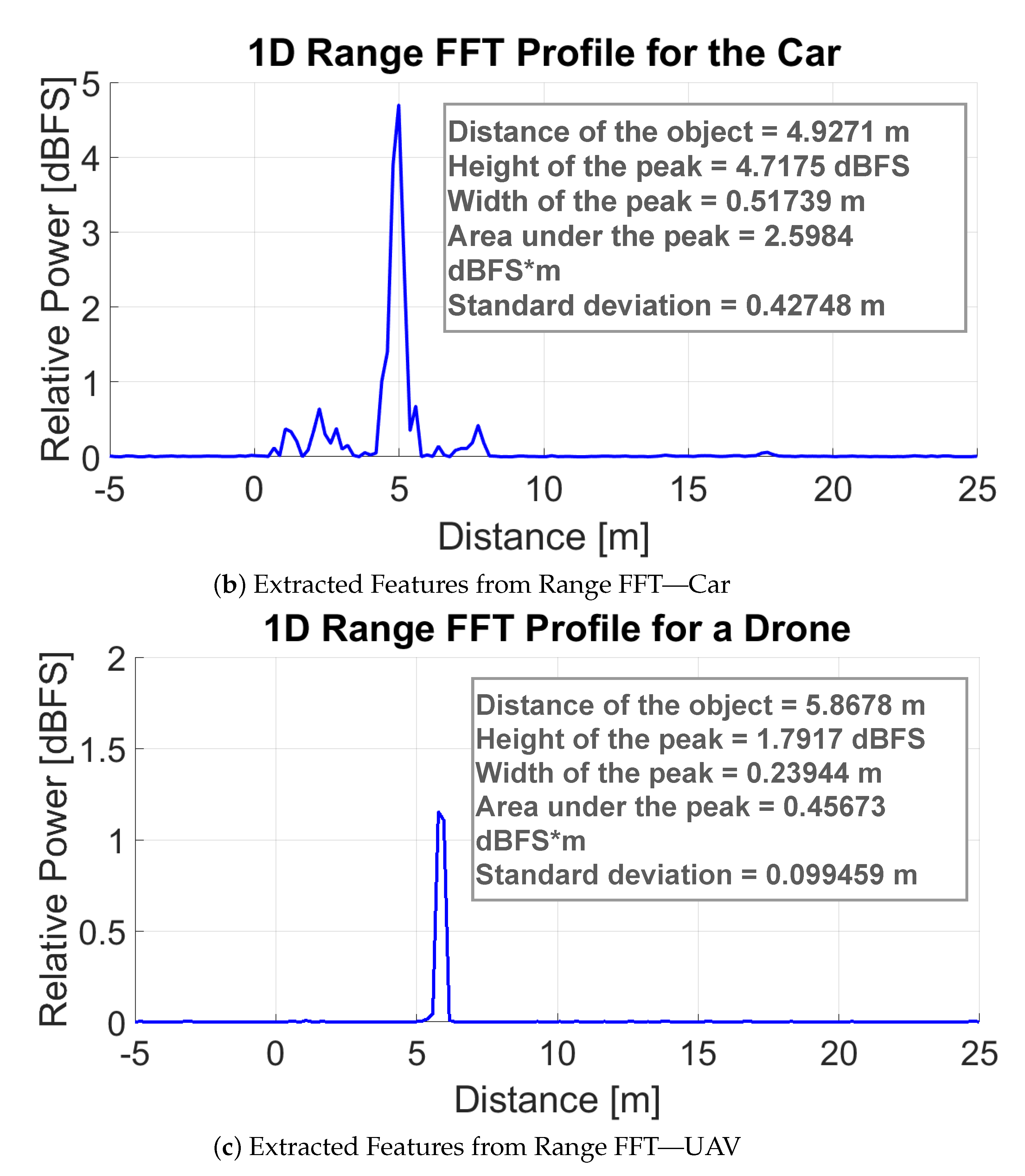
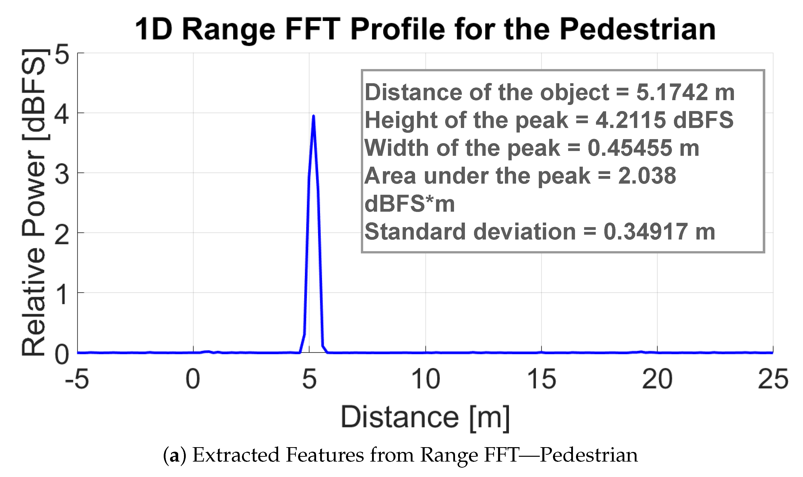
Figure 8 depicts a single outdoor measurement case for three targets: a car, a pedestrian, and an UAV (drone). According to Figure 8, the areas under the peak extracted from range FFT for a car, a pedestrian, and a drone are 2.5984, 2.038, and 0.45673, respectively. It is proportional to the cross-section of the targets. Similarly, peak height, standard deviation, and width are also proportional to the target features such as shape. All of these extracted features are further processed by using machine learning techniques for target classification.

4. Machine Learning Algorithms and Performance Evaluation

4.1. Models

A machine learning model is depicted in Figure 9. Each of the three classes has 226 samples in our data set. Each sample has five properties: the target’s radial range (m), the area under the peak (dBFS × m), the peak’s height (dBFS), the peak’s width(m), and the standard deviation (m) of the peak in the IF signal’s range FFT. The Human, Drone, and Car are the class labels.

Table 2. Per class total samples, train samples, and test samples count.

S. No.	Class	Total Number of Samples	Training Samples	Testing Samples
1	Human	95	86	10
2	Drone	59	53	6
3	Car	72	65	7
	Total	226	203	23

displays the sample count for each class.

The dataset is divided into two sections: training and testing. The training set consists of 90% of the samples of the total dataset. The testing set contains 10% of samples of the total dataset. Then, by using our dataset, we compare the performance, size, and other parameters of various machine learning models.

4.1.1. Logistic Regression

The probabilities for classification problems with two possible outcomes are modeled by using logistic regression. It is a classification-problem extension of the linear regression model. Logistic regression is a supervised ML model based on logistic function. This ML technique is useful to predict the binary decision variables {0,1}. There is only one node and two operations: (i) a linear combination of model parameters such as weights and bias and input (7); (ii) non-linear activation, which in this case is a sigmoid function (8). The model then computes the probability ‘p’ that it belongs to the specified class following the second operation [46]. The logistic regression model calculates the probability ‘p’ as shown in Equation (9). In (7), ‘w’ is the weight vector, and ‘x’ is one sample vector. In (9), ‘Y’ is the class label, and ‘X’ is the given dataset. In its most basic form, logistic regression is used to classify only two classes. A multi-class classification model is used as our dataset has three classes. For classification, we employ the one versus all method, also known as the one vs. rest method. By this approach, we generate ‘n’ classifiers associated with ‘n’ classes. We choose one class as class ‘0’ and all other classes as class ‘1’ from the dataset for each classifier. The logistic regression model is then used to distinguish between classes ‘0’ and ‘1’. The same procedure is used to process the remaining ‘n’ classifiers in the dataset [47]. The logistic regression model and its confusion matrix for our dataset ‘n’ = 3 is shown in Figure 10 and Figure 11 [48], respectively.

$$z=w^T\ast x_i$$

(7)

$$sig\left(z\right)=\frac{1}{1+e^{-z}}$$

(8)

$$p(Y/X)=sig\left(z\right)$$

(9)

4.1.2. Naive Bayes

Naive Bayes (NB) is a type of generative machine learning model. The discriminative models are designed to learn the probability distribution $P(y\mid x)$ given the input x and corresponding label y. The generative ML model, on the other hand, estimates the joint probability P(x,y) and applies the Bayes theorem to obtain $P(y\mid x)$. The NB algorithm is a popular supervised ML algorithm for dealing with classification problems. This algorithm is based on the assumption that features are conditionally independent of one another [49]. The NB algorithm has three variants based on the input features: (i) input with binary features; (ii) input with discrete features; and (iii) input with continuous features. For input of binary type features, Bernoulli NB is used, Multinomial NB is used for the input type of discrete features, and Gaussian NB is used for the input type of continuous features. We used the Gaussian NB model because our features were continuous. First, we computed the likelihood ratios from our dataset. Following that, the posterior probability for each class is computed as shown in (10). In (10), ‘Y’ is the class label, ‘X’ is the given dataset, ‘p(Y/X)’ is the conditional probability of ‘Y’ given ‘X’, and ‘p(X)’ is the marginal probability of ‘X’. The sample is a member of the class with the highest posterior probability. Figure 12 shows the Naive Bayes model. Figure 13 depicts the Naive Bayes model’s confusion matrix.

$$p(Y=C_i/X)=\frac{p(X/Y=C_i)\ast p(Y=C_i)}{p\left(X\right)}$$

(10)

4.1.3. Support Vector Machine (SVM)

The Support Vector Machine model was the next model we investigated for our dataset. By locating a hyperplane between the classes, this model generates a classifier. A hyperplane is a plane that separates two classes with the greatest possible margin. The classes are separable with both linear and non-linear methods. Hyper-planes are easily found in linearly separable cases. SVM uses a kernel to convert non-linearly separable classes to linearly separable classes by converting low dimension input space to higher dimension space [50]. The SVM model uses the Lagrangian method and dual problem formulation for the model’s optimization. The Lagrangian function and the dual problem formulation are shown in the (11) and (12). In (11) and (12), ‘w’ is the weight vector, ‘$\alpha$’ is the lagrangian multiplier, ‘$y_i$’ is the class label, ‘$x_i$’ is the given sample, ‘m’ is the total number of samples, and ‘b’ is the bias term. In (12), ‘K($x_i,x_j$)’ is the kernel term, and we used the ‘RBF’ kernel in this work as defined in Equation (13). In (13), ‘$\gamma$’ is called as the kernel coefficient. After calculating the optimal ‘w’ and ‘b’, the model classifies a sample using Equation (14). In its most basic form, SVM is a binary classification model. Thus, in order to make it work with our dataset, we used the one vs. all multi-class classification method described in the previous section. The model’s hyperparameter values are as follows: ‘C’ = 1.0 and ‘kernel’ = ‘rbf’. The SVM models and its confusion matrix are depicted in Figure 14 and Figure 15 respectively.

$$L(w,b,\alpha )=\frac{1}{2}\ast (w\ast w)-\sum _{i=1}^m{\alpha }_i\ast [y_i\ast (w\ast x_i+b)-1]$$

(11)

$$\begin{array}{c}\hfill \underset{\alpha }{max}\sum _{i=1}^m{\alpha }_i-\frac{1}{2}\ast (\sum _{i=1}^m\sum _{j=1}^m({\alpha }_i\ast {\alpha }_j\ast y_i\ast y_j\ast K(x_i,x_j))\\ \hfill \mathrm{subject}\mathrm{to}{\alpha }_i\ge 0,i=1,2\dots m,\sum _{i=1}^m{\alpha }_i\ast y_i=0\end{array}$$

(12)

$$K(x_i,x_j)=e^{(\gamma \ast ||x_i-x_j|{|}^2)}$$

(13)

$$h\left(x_i\right)=\left\{\begin{array}{cc}{C}_1,\hfill & \mathrm{if}w\ast x_i+b\ge 0\hfill \\ not C_1,\hfill & \mathrm{if}w\ast x_i+b<0\hfill \end{array}\right.$$

(14)

4.1.4. Light Gradient Boost Methods

The Light Gradient Boost method is the next machine learning model used (Light GBM). Light GBM is currently one of the most powerful performance enhancing algorithms available. A decision tree algorithm is used in this method. Unlike other boosting algorithms that divide the decision tree level-wise or depth-wise, Light GBM divides the decision tree leaf-wise. This leaf-wise split can reduce loss but can also result in overfitting. Since the model contains a hyper-parameter, it can control the depth of the tree for the leaf-wise split to avoid overfitting [51]. The split is made by calculating the residual value for each leaf as shown in Equation (15). Since we restrict the number of leaves that will be present, we cannot directly sum the residuals of all leaves, instead we uses the gradient boosting transformation technique shown in Equation (16). In Equation (16), ‘$\gamma$’ is the transformation value, ‘r’ is the residual of each leaf, and ‘p’ is the previous predicted probability for each residual. Thus, we transform the tree by this method. When compared to other machine learning algorithms, this model is extremely fast. This model is built with the available ‘lightgmb’ library. The following are the various hyper-parameter values for the model: ‘boosting type’ = ‘gbdt’; ‘objective’ = ‘multiclass’; ‘metric’ = ‘multi logloss’; ‘sub feature’ = 0.5; ‘num leaves’ = 10; ‘min data’ = 50; ‘max depth’ = 10; and ‘num class’ = 3. Figure 16 depicts LGBM model. Figure 17 depicts the confusion matrix for the Light GBM model on test data.

$$Residual=Observed\_Value-Predicted\_Value$$

(15)

$$\gamma =\frac{\sum \left(r\right)}{\sum (p\ast (1-p\left)\right)}$$

(16)

4.2. Performance Evaluation

On the test dataset, the performance of the four deployed models is compared using four evaluation metrics. Each of the evaluation metric consists of the following elements: ‘True Positive (TP)’, ‘True Negative (TN)’, ‘False Positive (FP)’ and ‘False Negative (FN)’ [52]. They are detailed below.

4.2.1. Accuracy

The accuracy [52] of all the four models along with their inference time and model size is shown in

Table 3. Accuracy of the four models, inference time, and model size. ms = Milli seconds; KB = Kilo Bytes.

S. No.	Model	Accuracy	Inference Time (ms)	Model Size (KB)
1	Naive Bayes	73.9%	0.24	1
2	Logistic Regression	86.9%	0.1	1
3	SVM	87%	0.27	10
4	Light GBM	95.6%	0.48	523

. The accuracy is calculated according to Equation (17). It can be observed from Table 3 that the LightGBM method provides the best accuracy of 95.6%. For all models, the inference time is under 0.5 ms.

$$\mathrm{Accuracy}=(TP+TN)/(TP+FP+TN+FN)$$

(17)

4.2.2. Recall

The recall [52] of all four models is shown in

Table 4. Recall.

Class	Naive Bayes	Logistic Regression	SVM	Light GBM
Car	1.00	0.86	1.00	1.00
Drone	1.00	1.00	1.00	1.00
Human	0.40	0.80	0.70	0.90

. The recall is calculated according to Eqaution (18). From the above table (Table 4), it can be observed that Light GBM model performs the best for all the classes.

$$\mathrm{Recall}=\left(TP\right)/(TP+FN)$$

(18)

4.2.3. Precision

The precision [52] metric for all the models is shown in

Table 5. Precision.

Class	Naive Bayes	Logistic Regression	SVM	Light GBM
Car	0.78	0.86	0.78	1.00
Drone	0.60	0.86	0.86	0.86
Human	1.00	0.89	1.00	1.00

. This metric is calculated according to Equation (19). It can be observed from the table that Light GBM model outperforms over all the other models for all the three classes.

$$\mathrm{Precision}=\left(TP\right)/(TP+FP)$$

(19)

4.2.4. F1-Score

The F1-score [52] metric is calculated and shown for all the models in

Table 6. F1-score.

Class	Naive Bayes	Logistic Regression	SVM	Light GBM
Car	0.88	0.86	0.88	1.00
Drone	0.75	0.92	0.92	0.92
Human	0.57	0.84	0.82	0.95

. This metric is calculated according to Equation (20). It can be observed from Table 6 that Light GBM model values are the best as compared to other models for all the classes.

$$\mathrm{F}1\text{-}\mathrm{score}=2\times (Recall\times Precision)/(Recall+Precision)$$

(20)

5. Conclusions

In order to identify targets by using mmWave FMCW radars, a novel classification technique based on statistical features from a range profile has been proposed. The proposed method should be extended to include long-range targets as well as targets of various types with different shapes and sizes. The range profile may lack distinguishable features for long-range targets and targets with small cross sections, necessitating additional signal processing before applying machine learning. In addition to the features presented here, micro-Doppler features and various time-frequency plots can be incorporated into models to effectively classify the targets if any of the targets have vibrating parts or repeating patterns. In order to improve the robustness of the classification technique, the range-Doppler and range-azimuth plot features can be incorporated into the model.

References

1. Kocić, J.; Jovičić, N.; Drndarević, V. Sensors and Sensor Fusion in Autonomous Vehicles. In Proceedings of the 2018 26th Telecommunications Forum (TELFOR), Belgrade, Serbia, 21–20 November 2018; pp. 420–425. [Google Scholar]
2. Cenkeramaddi, L.R.; Bhatia, J.; Jha, A.; Vishkarma, S.K.; Soumya, J. A survey on sensors for autonomous systems. In Proceedings of the 15th IEEE Conference on Industrial Electronics and Applications, Kristiansand, Norway, 9–13 November 2020. [Google Scholar]
3. Alonso, L.; Milanes, V.; Torre-Ferrero, C.; Godoy, J.; Pérez-Oria, J.; Pedro, T. Ultrasonic Sensors in Urban Traffic Driving-Aid Systems. Sensors 2011, 11, 661–673. [Google Scholar] [CrossRef]
4. Thing, V.L.L.; Wu, J. Autonomous Vehicle Security: A Taxonomy of Attacks and Defences. In Proceedings of the 2016 IEEE International Conference on Internet of Things (iThings) and IEEE Green Computing and Communications (GreenCom) and IEEE Cyber, Physical and Social Computing (CPSCom) and IEEE Smart Data (SmartData), Chengdu, China, 15–18 December 2016; pp. 164–170. [Google Scholar]
5. Jha, A.; Subedi, D.; Løvsland, P.-O.; Tyapin, I.; Cenkeramaddi, L.R.; Lozano, B.; Hovland, G. Autonomous Mooring towards Autonomous Maritime Navigation and Offshore Operations. In Proceedings of the IEEE Conference on Industrial Electronics and Applications (ICIEA), Kristiansand, Norway, 9–13 November 2020; pp. 1171–1175. [Google Scholar]
6. Stockton, N. Autonomous Vehicle Industry Remains Cool to Thermal Imaging. Available online: https://spie.org/news/thermal-infrared-for-autonomous-vehicles?SSO=1 (accessed on 19 June 2021).
7. Oh, B.S.; Guo, X.; Lin, Z. A UAV Classification System based on FMCW Radar Micro-Doppler Signature Analysis. Expert Syst. Appl. 2019, 132, 239–255. [Google Scholar] [CrossRef]
8. Kim, B.K.; Kang, H.; Park, S. Drone Classification Using Convolutional Neural Networks With Merged Doppler Images. IEEE Geosci. Remote Sens. Lett. 2017, 14, 38–42. [Google Scholar] [CrossRef]
9. Govoni, M.A. Micro-Doppler signal decomposition of small commercial drones. In Proceedings of the 2017 IEEE Radar Conference (RadarConf), Seattle, WA, USA, 8–12 May 2017; pp. 0425–0429. [Google Scholar]
10. Jian, M.; Lu, Z.; Chen, V.C. Drone detection and tracking based on phase-interferometric Doppler radar. In Proceedings of the 2018 IEEE Radar Conference (RadarConf18), Oklahoma City, OK, USA, 23–27 April 2018; pp. 1146–1149. [Google Scholar]
11. Pan, E. Object Classification Using Range-Doppler Plots from a High Density PMCW MIMO mmWave Radar System. Available online: http://hdl.handle.net/2142/107240 (accessed on 19 June 2021).
12. Gupta, S.; Rai, P.K.; Kumar, A.; Yalavarthy, P.K.; Cenkeramaddi, L.R. Target Classification by mmWave FMCW Radars using Machine Learning on Range-Angle Images. IEEE Sens. J. 2021, 1. [Google Scholar] [CrossRef]
13. Cho, M. A Study on the Obstacle Recognition for Autonomous Driving RC Car Using LiDAR and Thermal Infrared Camera. In Proceedings of the 2019 Eleventh International Conference on Ubiquitous and Future Networks (ICUFN), Zagreb, Croatia, 2–5 July 2019; pp. 544–546. [Google Scholar]
14. Subedi, D.; Jha, A.; Tyapin, I.; Hovland, G. Camera-LiDAR Data Fusion for Autonomous Mooring Operation. In Proceedings of the IEEE Conference on Industrial Electronics and Applications (ICIEA), Chengdu, China, 1–4 August 2020; pp. 1176–1181. [Google Scholar]
15. Kim, J.; Han, D.S.; Senouci, B. Radar and Vision Sensor Fusion for Object Detection in Autonomous Vehicle Surroundings. In Proceedings of the International Conference on Ubiquitous and Future Networks (ICUFN), Prague, Czech Republic, 3–6 July 2018; pp. 76–78. [Google Scholar]
16. Estl, H. Paving the Way to Self-Driving Cars with Advanced Driver Assistance Systems. Available online: https://www.mouser.cn/pdfdocs/sszy019-1.pdf (accessed on 19 June 2021).
17. Björklund, S.; Petersson, H.; Nezirovic, A.; Guldogan, M.B.; Gustafsson, F. Millimeter-wave radar micro-Doppler signatures of human motion. In Proceedings of the 2011 12th International Radar Symposium (IRS), Leipzig, Germany, 7–9 September 2011; pp. 167–174. [Google Scholar]
18. Singh, A.K.; Kim, Y.H. Analysis of Human Kinetics Using Millimeter-Wave Micro-Doppler Radar. Procedia Comput. Sci. 2016, 84, 36–40. [Google Scholar] [CrossRef] [Green Version]
19. Rahman, S.; Robertson, D. Time-Frequency Analysis of Millimeter-Wave Radar Micro-Doppler Data from Small UAVs. In Proceedings of the 2017 Sensor Signal Processing for Defence Conference (SSPD), London, UK, 6–7 December 2017; pp. 1–5. [Google Scholar]
20. Rahman, S.; Robertson, D.A. Radar micro-Doppler signatures of drones and birds at K-band and W-band. Sci. Rep. 2018, 8, 17396. [Google Scholar] [CrossRef]
21. Fairchild, D.; Narayanan, R. Classification of human motions using empirical mode decomposition of human micro-doppler signatures. IET Radar Sonar Navig. 2014, 8, 425–434. [Google Scholar] [CrossRef]
22. Vandersmissen, B.; Knudde, N.; Jalalvand, A.; Couckuyt, I.; Bourdoux, A.; De Neve, W.; Dhaene, T. Indoor Person Identification Using a Low-Power FMCW Radar. IEEE Trans. Geosci. Remote Sens. 2018, 56, 3941–3952. [Google Scholar] [CrossRef] [Green Version]
23. Chen, V.C.; Li, F.; Ho, S.; Wechsler, H. Micro-Doppler effect in radar: Phenomenon, model, and simulation study. IEEE Trans. Aerosp. Electron. Syst. 2006, 42, 2–21. [Google Scholar] [CrossRef]
24. Clemente, C.; Balleri, A.; Woodbridge, K.; Soraghan, J.J. Developments in target micro-Doppler signatures analysis: Radar imaging, ultrasound and through-the-wall radar. Eurasip J. Adv. Signal Process. 2013, 2013, 47. [Google Scholar] [CrossRef] [Green Version]
25. Montgomery, D.; Holmén, G.; Almers, P.; Jakobsson, A. Surface Classification with Millimeter-Wave Radar Using Temporal Features and Machine Learning. In Proceedings of the 2019 16th European Radar Conference (EuRAD), Paris, France, 2–4 October 2019; pp. 1–4. [Google Scholar]
26. Molchanov, P.; Egiazarian, K.; Astola, J.; Harmanny, R.I.A.; de Wit, J.J.M. Classification of small UAVs and birds by micro-Doppler signatures. In Proceedings of the 2013 European Radar Conference, Nuremberg, Germany, 9–11 October 2013; pp. 172–175. [Google Scholar]
27. Huizing, A.; Heiligers, M.; Dekker, B.; de Wit, J.; Cifola, L.; Harmanny, R. Deep Learning for Classification of Mini-UAVs Using Micro-Doppler Spectrograms in Cognitive Radar. IEEE Aerosp. Electron. Syst. Mag. 2019, 34, 46–56. [Google Scholar] [CrossRef]
28. Zhang, W.; Li, G. Detection of multiple micro-drones via cadence velocity diagram analysis. Electron. Lett. 2018, 54, 441–443. [Google Scholar] [CrossRef]
29. Fuhrmann, L.; Biallawons, O.; Klare, J.; Panhuber, R.; Klenke, R.; Ender, J. Micro-Doppler analysis and classification of UAVs at Ka band. In Proceedings of the 2017 18th International Radar Symposium (IRS), Prague, Czech Republic, 28–30 June 2017; pp. 1–9. [Google Scholar] [CrossRef]
30. Zhao, Y.; Su, Y. The Extraction of Micro-Doppler Signal With EMD Algorithm for Radar-Based Small UAVs’ Detection. IEEE Trans. Instrum. Meas. 2020, 69, 929–940. [Google Scholar] [CrossRef]
31. Zhao, Y.; Su, Y. Cyclostationary Phase Analysis on Micro-Doppler Parameters for Radar-Based Small UAVs Detection. IEEE Trans. Instrum. Meas. 2018, 67, 2048–2057. [Google Scholar] [CrossRef]
32. Ren, J.; Jiang, X. Regularized 2-D complex-log spectral analysis and subspace reliability analysis of micro-Doppler signature for UAV detection. Pattern Recognit. 2017, 69, 225–237. [Google Scholar] [CrossRef]
33. Regev, N.; Yoffe, I.; Wulich, D. Classification of single and multi propelled miniature drones using multilayer perceptron artificial neural network. In Proceedings of the International Conference on Radar Systems (Radar 2017), Belfast, UK, 23–26 October 2017; pp. 1–5. [Google Scholar] [CrossRef]
34. Song, H.; Shin, H. Classification and Spectral Mapping of Stationary and Moving Objects in Road Environments Using FMCW Radar. IEEE Access 2020, 8, 22955–22963. [Google Scholar] [CrossRef]
35. Palffy, A.; Kooij, J.; Gavrila, D. CNN based Road User Detection using the 3D Radar Cube. IEEE Robot. Autom. Lett. 2020, 5, 1263–1270. [Google Scholar] [CrossRef] [Green Version]
36. Stadelmayer, T.; Stadelmayer, M.; Santra, A.; Weigel, R.; Lurz, F. Human Activity Classification Using Mm-Wave FMCW Radar by Improved Representation Learning. In Proceedings of the 4th ACM Workshop on Millimeter-Wave Networks and Sensing Systems, mmNets’20, London, UK, 25 September 2020; Association for Computing Machinery: New York, NY, USA, 2020. [Google Scholar] [CrossRef]
37. Li, X.; He, Y.; Jing, X. A Survey of Deep Learning-Based Human Activity Recognition in Radar. Remote Sens. 2019, 11, 1068. [Google Scholar] [CrossRef] [Green Version]
38. Bhatia, J. Object Classification Technique for mmWave FMCW Radars using Range-FFT Features. In Proceedings of the International Conference on Communication Systems and Networks (COMSNETS 2021), Bangalore, India, 5–9 January 2020. [Google Scholar]
39. Dayal, A. Radar_classification. Available online: https://github.com/aveen-d/Radar_classification (accessed on 19 June 2021).
40. The Fundamentals of Millimeter Wave Sensors. Available online: https://www.mouser.ee/pdfdocs/mmwavewhitepaper.pdf (accessed on 19 June 2021).
41. Sanoal, M.; Santiago, M. Automotive FMCW Radar Development and Verification Methods. Master’s Thesis, Department of Computer Science and Engineering, Chalmers University of Technology, Gothenburg, Sweden, 2018. Available online: https://hdl.handle.net/20.500.12380/255195 (accessed on 19 June 2021).
42. Ding, Y.; Huang, G.; Hu, J.; Li, Z.; Zhang, J.; Liu, X. Indoor Target Tracking Using Dual-Frequency Continuous-Wave Radar Based on the Range-Only Measurements. IEEE Trans. Instrum. Meas. 2020, 69, 5385–5394. [Google Scholar] [CrossRef]
43. Gao, Y.; Qaseer, M.T.A.; Zoughi, R. Complex Permittivity Extraction From Synthetic Aperture Radar Images. IEEE Trans. Instrum. Meas. 2020, 69, 4919–4929. [Google Scholar] [CrossRef]
44. González-Díaz, M.; García-Fernández, M.; Álvarez-López, Y.; Las-Heras, F. Improvement of GPR SAR-Based Techniques for Accurate Detection and Imaging of Buried Objects. IEEE Trans. Instrum. Meas. 2020, 69, 3126–3138. [Google Scholar] [CrossRef] [Green Version]
45. Gallion, J.R.; Zoughi, R. Millimeter-Wave Imaging of Surface-Breaking Cracks in Steel With Severe Surface Corrosion. IEEE Trans. Instrum. Meas. 2017, 66, 2789–2791. [Google Scholar] [CrossRef]
46. Berger, D. Introduction to Binary Logistic Regression and Propensity Score Analysis. Available online: https://www.researchgate.net/publication/320505159_Introduction_to_Binary_Logistic_Regression_and_Propensity_Score_Analysis (accessed on 19 June 2021).
47. Rifkin, R.; Klautau, A. In Defense of One-Vs-All Classification. J. Mach. Learn. Res. 2004, 5, 101–141. [Google Scholar]
48. Ting, K.M. Confusion Matrix. In Encyclopedia of Machine Learning and Data Mining; Sammut, C., Webb, G.I., Eds.; Springer: Boston, MA, USA, 2017; p. 260. [Google Scholar] [CrossRef]
49. Berrar, D. Bayes’ Theorem and Naive Bayes Classifier. In Encyclopedia of Bioinformatics and Computational Biology; Elsevier Science Publisher: Amsterdam, The Netherlands, 2019; pp. 403–412. [Google Scholar] [CrossRef]
50. Awad, M.; Khanna, R. Support Vector Machines for Classification; Apress: Berkeley, CA, USA, 2015; pp. 39–66. [Google Scholar] [CrossRef] [Green Version]
51. Ke, G.; Meng, Q.; Finley, T.; Wang, T.; Chen, W.; Ma, W.; Ye, Q.; Liu, T.Y. LightGBM: A Highly Efficient Gradient Boosting Decision Tree. In Proceedings of the 31st International Conference on Neural Information Processing Systems, NIPS’17, Long Beach, CA, USA, 4–9 December 2017; Curran Associates Inc.: Red Hook, NY, USA, 2017; pp. 3149–3157. [Google Scholar]
52. Ghori, K.M.; Abbasi, R.A.; Awais, M.; Imran, M.; Ullah, A.; Szathmary, L. Performance Analysis of Different Types of Machine Learning Classifiers for Non-Technical Loss Detection. IEEE Access 2020, 8, 16033–16048. [Google Scholar] [CrossRef]
Figure 1. System level diagram.
Electronics 10 01965 g001
Figure 2. Radar front-end architecture with complex IF signal.
Electronics 10 01965 g002
Figure 3. FMCW signal pattern.
Electronics 10 01965 g003
Figure 4. Details of frame structure.
Electronics 10 01965 g004
Figure 5. Features extraction flow chart.
Electronics 10 01965 g005
Figure 6. Measurement Setup.
Electronics 10 01965 g006
Figure 7. Extracted Features Plot.
Electronics 10 01965 g007
Figure 8. Features extracted in the range FFT profile.
Electronics 10 01965 g008aElectronics 10 01965 g008b
Figure 9. Overview of machine learning model.
Electronics 10 01965 g009
Figure 10. Logistic regression model.
Electronics 10 01965 g010
Figure 11. Logistic regression model’s confusion matrix on test data.
Electronics 10 01965 g011
Figure 12. Naive Bayes Model.
Electronics 10 01965 g012
Figure 13. Confusion matrix of Naive Bayes model on test data.
Electronics 10 01965 g013
Figure 14. Support Vector Machine Model.
Electronics 10 01965 g014
Figure 15. Confusion matrix of SVM model on test data.
Electronics 10 01965 g015
Figure 16. Light Gradient Boost Methods Model.
Electronics 10 01965 g016
Figure 17. Confusion matrix of LightGBM model on test data.
Electronics 10 01965 g017