Dynamic Target Tracking and Ingressing of a Small UAV Using Monocular Sensor Based on the Geometric Constraints

Abstract

In many applications of airborne visual techniques for unmanned aerial vehicles (UAVs), lightweight sensors and efficient visual positioning and tracking algorithms are essential in a GNSS-denied environment. Meanwhile, many tasks require the ability of recognition, localization, avoiding, or flying pass through these dynamic obstacles. In this paper, for a small UAV equipped with a lightweight monocular sensor, a single-frame parallel-features positioning method (SPPM) is proposed and verified for a real-time dynamic target tracking and ingressing problem. The solution is featured with systematic modeling of the geometric characteristics of moving targets, and the introduction of numeric iteration algorithms to estimate the geometric center of moving targets. The geometric constraint relationships of the target feature points are modeled as non-linear equations for scale estimation. Experiments show that the root mean square error percentage of static target tracking is less than 1.03% and the root mean square error of dynamic target tracking is less than 7.92 cm. Comprehensive indoor flight experiments are conducted to show the real-time convergence of the algorithm, the effectiveness of the solution in locating and tracking a moving target, and the excellent robustness to measurement noises.

1. Introduction

With the rapid development of UAV system technologies and the increasing demands for UAVs to perform various aerial tasks [1,2,3,4], UAVs employ airborne vision sensors to achieve the goal of autonomous target tracking and positioning [5,6,7,8]. Over the past ten years, the related technologies for UAVs have received more and more attention from both academic and industrial researchers in the fields of computer vision and artificial intelligence [9,10,11,12]. There are still many challenges towards autonomous quadrotor flight in complex environments, which are flying through windows, narrow gaps, and dynamic opening entries [13,14,15]. Many high-level competitions of UAVs also pay great attention to scenes, such as dynamic target tracking and multiple coordinated UAVs crossing the door-like targets.

In the past, radio navigation schemes were often used for the positioning and tracking of UAVs [16]. However, with the development of visual equipment and computer vision algorithms, visual navigation and tracking have gradually attracted the attention of experts in this field. The visual sensor-based methods for UAV target tracking can be generally divided into three types. The first type is to combine the measurements from the RGB camera and depth sensors, directly generating the depth information of the target and realizing the direct positioning of the target [17,18]. Although the positioning accuracy of this type may be satisfactory, it depends on the capability of larger sensor load and high-cost computation unit (to ensure the real-time performance) and, thus, is not suitable for the applications to low-cost small UAVs. The second type is to use various visual features of the target image to carry out affine transformation and feature points matching, and then construct motion constraint equations and bundle iterative optimization [19] for multi-frame images [20,21,22] to realize the solution of posture trajectory of the target space. The solutions of this type often rely on binocular vision, possibly leading to higher computing complexity and smaller measuring range. The third category is to use the monocular visual method to solve the depth estimation of targets, to realize the target positioning and tracking. The leading-edge monocular simultaneous localization and mapping (SLAM) using the visual-inertial navigation framework has been proposed and effectively solved the problem of scale ambiguity by using the characteristic of the inertial sensor [23,24,25,26]. Additionally, mainstream methods include using height information to estimate scale values [27], combining the 3D map with edge alignment methods [28], and using deep neural network algorithms to estimate pixels’ depth values [29,30]. However, these solutions highly depend on the accuracy of the inertial navigation device or height sensor, or require the three-dimensional map information, or need offline templates or a high computing budget for online learning, etc.

Motivated by the above observations, we aim to develop a fast and high-accuracy visual tracking solution for a small UAV equipped with a low-cost tiny monocular vision sensor. In practice, when the tracking algorithm is initialized, we use the inertial navigation units and multi-frame images obtained by the monocular camera to obtain the scale of our targets. After that, we use the tracking-by-detection method to realize the tracking of single-frame parallel features. The main technical contributions of this paper are summarized as follows:

• Aiming at the problem of tracking dynamic targets, a single-frame parallel-features positioning method (SPPM) is proposed. Compared with a standard solution to the perspective 3 points problem of moving targets, our method extracts the coplanar parallel constraint relations between target feature points to construct high-order non-linear over-determined equations with unknown depth values. Then, we introduced an improved Newton numerical optimization based on the Runge–Kutta method, which greatly reduces the error caused by 2D detection in UAVs’ actual engineering applications. In our experiments, after randomly increasing the 2D point error within three pixels, SPPM can still guarantee the 3D positioning error within 1.10%. Experimental results show that SPPM is robust to 2D detection errors and in the presence of detection noise;
• Based on the SPPM, a 2D feature recognition algorithm for parallel feature extraction was designed. Then, we introduced a monocular SLAM algorithm based on PTAM for navigation. Finally, an indoor UAV visual positioning and tracking framework that integrates target feature recognition, monocular SLAM positioning, and dynamic target tracking was constructed;
• To verify the effectiveness and robustness of the framework, we have carried out several indoor flight test experiments for a small UAV AR. DRONE2.0 [31] to track, and the UAV is equipped with a lightweight monocular camera as the visual front-end which is shown in Figure 1. Combining our SPPM and our intelligent monocular SLAM navigation platform [32], a complete indoor autonomous navigation and positioning system is proposed. Our method is systematically evaluated by considering the computation amount, the convergence speed of the depth value, and the tracking accuracy. In the actual flight test, the average number of iterations of the depth estimation equations is only 1.94 for visual data with the resolution of $640\times 360$. The UAV can fly through the center of the door frame successfully, and the root mean square errors (RMSE) of the dynamic target is smaller than 7.92 cm.

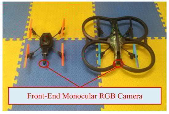Figure 1. Parrot AR. DRONE2.0.

The rest of the paper is organized as follows. Section 2 analyzes the requirements of the core algorithm and describes related mathematical knowledge. Section 3 describes the framework and the mathematical model of the target tracking algorithm in this paper. Section 4 describes the construction of the experimental system and several indoor experiments and analyzes the detailed experimental results. Section 5 summarizes the algorithm framework of this paper and some future research directions are pointed out. The following part mentions the source of funding for our research. The videos of some key elements of the indoor experiments have been uploaded. The link to access the videos of the indoor flight tests is: https://www.youtube.com/channel/UCffskCQrtyqhfiwE0xPGZKA/ (accessed on 15 July 2020).

2. Background and Preliminaries

2.1. Applicable Scene and Key Technologies

In the problem of UAV dynamic target tracking, both the flight platform and the target are dynamic. The motion characteristics of the dynamic target are random and continuous, so the numerical iteration method can make the initial value of iteration close to the numerical solution while estimating the next position, and accelerate the iteration speed. The feature points positioning in traditional SLAM methods are often based on static feature points, which are not suitable for moving targets. It is also worth noting that the SLAM scheme mainly uses static features to realize the positioning of the moving platform itself, and the tracking iteration speed for dynamic feature points is relatively slow. Therefore, the iterative solution of geometric constraint equations is more efficient.

This paper aims at the problem of UAV online real-time target positioning and tracking without GNSS signals, and studies how to realize the efficient, real-time, and stable positioning and tracking technology of UAV. We developed the capability for UAV of successfully ingressing through the dynamic openings or door-like windows of the target structure. The versatility of the algorithm framework is reflected in its application to visually relevant application scenarios, such as positioning, tracking, obstacle avoidance, and traversal of semi-cooperative targets for both indoor and outdoor environments. The key issues to be discussed in the paper are described as follows:

• Autonomous navigation: The fusion information of the visual sensor and the inertial navigation device is used to complete the estimation of the pose of the UAV without GNSS signals, and provide basic navigation information for subsequent flight missions;
• Target recognition: The door-like targets are analyzed, the parallel feature points of the target are extracted, and the target tracking of the two-dimensional plane is realized;
• Target 3D positioning: The key issue we consider in this article is to solve the 3D space position from the 2D point image feature. One mainstream solution is to use inertial navigation or binocular to solve epipolar geometry which is also called triangulation, and the other popular solution is to use depth neural to estimate the depth information of the image. However, these methods often require auxiliary sensors such as inertial navigation devices or several frames of image data for a joint solution.

Considering that this article discusses the spatial positioning and tracking of dynamic targets, we are trying to effectively use the geometric constraints of the target and the camera pose to solve the spatial position of the target within only one frame. The target features are abstracted with the geometric model, then the three-dimensional projection model and depth constraint equations are constructed. Additionally, the position of the geometric center of the target in the world coordinate system in the single-frame image is solved. Finally, the three-dimensional space positioning and tracking of the target are realized.

2.2. Background of 2D Target Tracking

At present, there have been a large number of research methods and theories for 2D tracking, such as morphological tracking [33,34], template-based tracking [35,36], kernelized correlation filters method [37], compressed sensing method [38,39], deep-learning-based tracking [40,41], etc. The targets involved in this article have relatively fixed geometric characteristics. Taking into account the reduction in the on-board computing pressure of the small UAV, a combination of morphological algorithm and tracking-by-detection method was adopted.

2.3. Mathematical Preliminaries

2.3.1. Coordinate System

The main coordinate systems involved in the UAV navigation are shown in Figure 2 and described as follows:

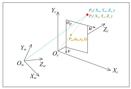
Figure 2. Diagram of coordinate systems.

• The world coordinate system: The absolute coordinate system with the fixed objective world. The world coordinate system is often used as the benchmark coordinate system to describe the spatial position of the target we are tracking, which is expressed by $P_w={[X_w{,Y}_w{,Z}_w]}^T$;
• The pixel coordinate system $\mathit{UV}$: The center of the image plane is taken as the coordinate origin, and the axis $X$ and axis $Y$ are parallel to the two vertical sides of the image plane, respectively, which is expressed by $P_{uv}={[u_x{v}_{y}1]}^T$. It is used to describe the 2D projection position of the target;
• The camera coordinate system $C$: The optical center of the camera is taken as the coordinate origin, the axis $X$ and axis $Y$ are parallel to the axis $X$ and axis $Y$ of the image coordinate system respectively, and the optical axis of the camera is the axis $Z$, which is expressed by $P_c={[X_c{Y}_c{Z}_c]}^T$.

Figure 2 shows the relationship between the three coordinate systems, where blue, green, and orange represent projections under the world coordinate system, camera coordinate system, and pixel coordinate system, respectively.

2.3.2. Camera Projection Model

For the target tracking problem of UAVs, the vision sensor is fixed on the platform of UAVs, and the target is described as 2D coordinates in the pixel coordinate system of the camera. Using the camera model and projection equations, the 2D coordinates can be projected into the target position in the camera coordinate system, see Equation (1).

$$p_{uv}=\frac{1}{Z_c}\cdot K{P}_c$$

(1)

where $K$ represents the internal parameter matrix of the camera model. Then, we can use the rotation and translation of the camera relative to the world coordinate system to obtain the pose of the target in the world coordinate system.

This paper mainly discusses the pinhole-like model with distortion characteristics, also known as the arctangent (ATAN) camera projection model [42]. This model can be widely used in most monocular color cameras on the market. Similarly, the projection equation of the pinhole projection model can be easily derived through this model. The specific mathematical model of ATAN projection will be expounded in combination with the algorithm in Section 3.

2.3.3. Numerical Newton Iteration Method

The Newton method in optimization is to use the iteration method to solve the optimal solution of a function. The traditional Newton iteration method has the characteristics of second-order convergence and accurate solution. The iterative equation is as follows:

$$X^{n+1}=X^n-{\nabla }^{2}F{(X)}^{-1}\cdot \nabla F\left(X\right)$$

(2)

For our algorithm, $X$ is the vector space of the unknown depth value to be solved in our algorithm, $\nabla F\left(X\right)$ is the Jacobian derivative matrix and ${\nabla }^{2}F{(X)}^{-1}$ is the inverse matrix of the Hessian matrix. However, the traditional Newton iterative optimization has a large amount of calculation when calculating the inverse matrix of the Hessian matrix, and the second derivative may fall into the endless loop at the inflection point, i.e., $f^{″}\left(x_n\right)=0$.

In this paper, an improved Newton–Raphson method with higher-order convergence is adopted [43,44,45], which possesses the advantages of fast convergence speed, fewer iteration times, and a high-efficiency evaluation index $R_e$. Another advantage is that it avoids the calculation of the Hessian matrix. Due to its high-order convergence, it can prevent the second derivative from falling into the iterative endless loop when there is an inflection point. The method can also effectively reduce the number of iterations together with the geometric constraint equation constructed by us later.

2.3.4. Generalized Inverse Matrix and Singular Value Decomposition

Considering that the equations solved by this algorithm in this paper may be overdetermined, that is, the number of equations is greater than the number of the unknowns, it is necessary to find the generalized inverse matrix $F^{+}$ of $F$. The purpose of constructing the generalized inverse matrix is to find a matrix similar to the inverse matrix for the non-square matrix. The generalized inverse matrix can be solved by singular value decomposition. For a real nonlinear coefficient matrix $F\in R^{m\times m}$, the generalized inverse matrix $F^{+}$ is:

$$F^{+}=U\cdot \Sigma \cdot V^T$$

(3)

where $U\in R^{m\times m}$ and $V\in R^{n\times n}$ are unit orthogonal matrixes, and $\Sigma \in R^{m\times n}$ only has values on the main diagonal which is called singular value matrix. Similar matrix inversion methods are widely used in engineering [46,47].

3. Framework of Tracking Algorithm

3.1. Overall Framework and Mathematical Models

For a small UAV to track a visual moving target in the GNSS-denied environment, the dynamic target positioning and tracking algorithm framework shown in Figure 3. The part in the dashed box is the core algorithm of the SPPM.

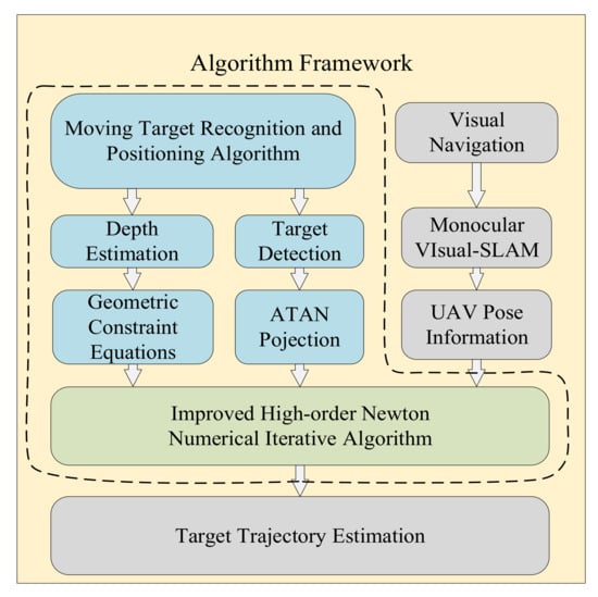
Figure 3. Diagram of the overall framework.

The framework is mainly concerned with the developments of the following three models:

• Monocular visual SLAM model: In this paper, the UAV target tracking is based on the monocular vision, so a monocular vision SLAM method is introduced as the positioning algorithm for the UAV, which can save cost and improve the system design compactness. Additionally, because of the common visual load, it is more convenient for researchers to carry out data processing and synchronization. The camera pose provided by this model will be used to calculate the world coordinates of the target. The pose calculation is used as an input to our core algorithm (SPPM). Therefore, in this article, we will not perform in-depth research in mono-SLAM;
• Two-dimensional target detection and camera projection model: In this paper, the traditional target detection algorithm is used to ensure the real-time performance of the detection module. Considering the generality, two projection models of the pinhole camera and the ATAN camera can both adapt to our subsequent algorithm. This paper focuses on the ATAN projection model, and the pinhole model can be regarded as a simplify case. The camera calibration method in this article refers to the calibration method for the FOV model camera which is also called the arctangent (ATAN) model in the ethzasl_ptam project of the ETH Zurich autonomous systems lab (ASL). This method applies to both global shutter and rolling shutter cameras. For specific methods, please refer to the official GitHub website of autonomous systems lab: https://github.com/ethz-asl/ethzasl_ptam (accessed on 12 July 2021);
• Three-dimensional monocular depth estimation and positioning model: The depth information solution also called the scale calculation problem, is one of the key problems in the target positioning and tracking technology based on the monocular vision. In this paper, the camera projection model and geometric constraint equations are used to construct the depth equations model. The target is abstracted as a rectangle or a parallelogram, and the improved high-order Newton iterative algorithm is used to realize the efficient real-time numerical solution of the depth information of the target feature points. Finally, the Kalman filter and linear regression are used to filter and estimate the target trajectory.

3.2. Extraction of Two-Dimensional Feature Points

The input of the two-dimensional feature extraction module is the UAV image information, and the output is the pixel coordinates of the feature points. The algorithm framework of the model is shown in the Figure 4 below:

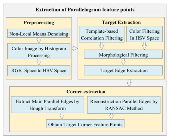
Figure 4. Framework of 2D feature extraction.

In this paper, the target features are abstracted as common geometric images, and the corner or inflection point of the target is abstracted with the color and shape features of the semi-cooperative target. The main part of the algorithm is as follows:

• Pre-processing: The visual information of AR. Drone2.0 is processed for noise removal, color enhancement processing, and then the RGB color space is converted into the HSV color space. Preprocessing work is to improve the image quality of the monocular camera to a certain extent and facilitate the subsequent modules to perform related filtering processing;
• Target extraction: The shape template or color filter of the target can be selected for target recognition and extraction. Then, use the open operation in morphology to denoise the target edge. Finally, use the edge extraction function in OpenCV2.0 to obtain the edge vector information of the target;
• Corner extraction: After obtaining the edge vector, Hough transform was used to obtain the sides of the quadrilateral target or use the random sample consensus (RANSAC) [48] algorithm to re-estimate the sides of the target. The use of the RANSAC algorithm takes into account the partial lack of target edge information caused by illumination or occlusion, and the RANSAC algorithm can be used to reconstruct the target edges. Finally, the 2D coordinates of each vertex of the target can be obtained by calculating the intersection of each side. Figure 5a–d, with the door frame detection as an example, illustrate the specific process of target identification and feature corner extraction. The target detection algorithm used in this paper is characterized by fast and real-time performance, but it may have a slight pixel detection error which is usually within 1 to 2 pixels.

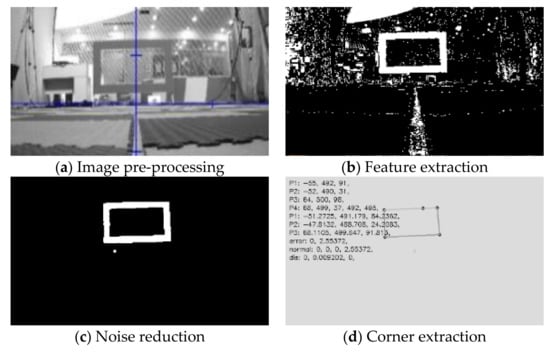Figure 5. Diagram of target corner extraction.

After the two-dimensional information is obtained, a three-dimensional depth estimation for the target was needed to conduct. The depth estimation problem is divided into two levels. Firstly, the basic problem of target depth estimation is to accurately solve the problem without considering the pixel error of two-dimensional detection. Furthermore, the robustness of target depth estimation with noise error in two-dimensional detection in actual engineering applications is considered. In the following experiments, it can be found that our algorithm framework is still robust when there is detection noise in two-dimensional feature points. Our algorithm can still estimate the target depth well in case of manual addition of 2–3 pixels for random detection of noise.

3.3. Depth Estimation and 3D Locating

The input of the depth estimation module is a known camera ATAN projection model and the pixel coordinates of the feature points, and the output is the depth estimation equations with the depth information of feature points as the unknown number. In this paper, the target features are abstracted as corners of concise geometric figures on the plane, as shown in Figure 6. The coordinates of the target in the world coordinate system are defined as $\mathrm{Pi}={[X_{\mathit{wi}}{,Y}_{\mathit{wi}}{,Z}_{\mathit{wi}}]}^T,i=1,2,3,4$. The coordinates in the UAV front-end monocular camera coordinate system are defined as $P_{w}i={[p_{wxi}{p}_{wyi}{p}_{wzi}]}^T,i=1,2,3,4$. The coordinates of the target in the two-dimensional image coordinate system are defined as $P_{uv}i={[u_i{v}_{i}1]}^T,i=1,2,3,4$. The normalized projection points of the normalized plane $Z=1$ are defined as $P_{c}i={[p_{cxi}{p}_{cyi}1]}^T,i=1,2,3,4.$

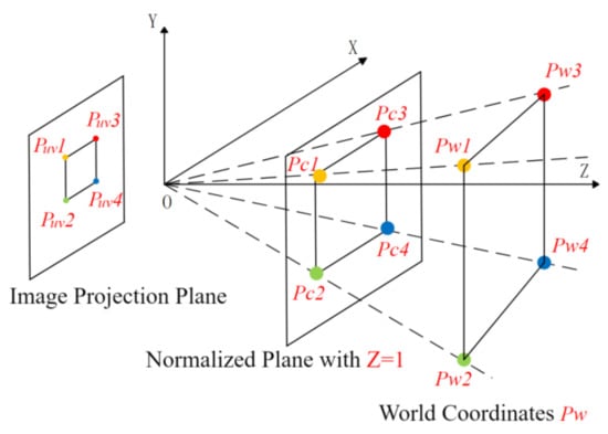
Figure 6. Schematic diagram of projection plane.

The ATAN projection model can be regarded as the superposition of the pinhole projection model and the FOV distortion model. Given the projection coordinates $X_c={[x_c{y}_c{z}_c]}^T$ on the normalized plane of the camera, the distortion radius $r_d$ is:

$$r_d=\frac{1}{\omega }\mathit{arctan}\left(2\cdot r\cdot \mathit{tan}\left(\frac{\omega }{2}\right)\right)$$

(4)

where $\omega$ is the camera distortion parameter. The distortion free projection radius $r$ is as follows:

$$r=\sqrt{\frac{x_c^2+y_c^2}{z_c^2}}=\sqrt{\frac{x_c^2+y_c^2}{1^2}}=\sqrt{x_c^2+y_c^2}$$

(5)

$\left[x_d{y}_d{z}_d\right]$ are the projection coordinates of distortion point:

$$\left\{\begin{array}{c}{x}_d=\frac{r_d}{r}\cdot x_c\\ y_d=\frac{r_d}{r}\cdot y_c\end{array}\right.\Rightarrow \left\{\begin{array}{c}{x}_d{}^2={(\frac{r_d}{r}\cdot x_c)}^2\\ y_d{}^2={(\frac{r_d}{r}\cdot y_c)}^2\end{array}\right.$$

(6)

$$x_d{}^2{+y}_d{}^2=\frac{r_d{}^2}{r^2}{(x_c{+y}_c)}^2$$

(7)

Additionally, from Equation (5) we can obtain:

$$\sqrt{x_d{}^2{\mathit{+}\mathit{y}}_d{}^2}{=r}_d$$

(8)

The relationship between the image coordinate system and the camera coordinate system can be obtained with the internal reference model of the pinhole camera:

$$\left[\begin{array}{l}u\\ v\\ 1\end{array}\right]=CM\cdot \left[\begin{array}{l}{x}_d\\ y_d\\ 1\end{array}\right]=\left[\begin{array}{l}{f}_{x}0c_x\\ 0f_x{c}_y\\ 001\end{array}\right]\left[\begin{array}{l}{x}_d\\ y_d\\ 1\end{array}\right]$$

(9)

where $CM$ is the internal parameter matrix. $CM$ and $\omega$ can be obtained by calibration of the ATAN camera model.

According to Figure 5, the UAV can identify target feature points and obtain a set of 2D image point positions through real-time image processing. We can obtain the coordinates of the projection with distortion $P_{c}i={[p_{cxi}{p}_{cyi}1]}^T$ in case of $Z=1$ plane by using the internal reference ATAN projection relationship.

$$P_{c}i=C{M}^{-1}\cdot P_{uv}i\cdot \frac{r}{r_d}$$

(10)

where $P_{c}i$ is the projection on the normalized plane $Z=1$, we can obtain:

$$P_{uv}i=\left[\begin{array}{l}{u}_{xi}\\ v_{yi}\\ 1\end{array}\right]=CM\cdot {\left[\frac{p_{wxi}}{p_{wzi}}\frac{p_{yxi}}{p_{wzi}}1\right]}^T$$

(11)

$$P_{c}i=\left[\begin{array}{c}{p}_{cxi}\\ p_{cyi}\\ p_{czi}\end{array}\right]={\left[\frac{p_{wxi}}{p_{wzi}}\frac{p_{wyi}}{p_{wzi}}1\right]}^T$$

(12)

Since $P_{c}i$ has been obtained from (10), we obtain the mathematical constraint relationship of $p_{wxi},p_{wyi},p_{wzi}$ in the feature point of $P_{w}i={[p_{wxi}{p}_{wyi}{p}_{wzi}]}^T$:

$$\left\{\begin{array}{c}{p}_{wxi}=p_{cxi}\cdot p_{wzi}\\ p_{wyi}=p_{cyi}\cdot p_{wzi}\end{array}\right.$$

(13)

The solution $p_{wzi}$ is to solve the scale $\lambda$ uncertainty problem in monocular vision positioning. So far, through formula (14), we can express $P_{w}i$ as a three-dimensional vector with only one unknown quantity $p_{wzi}$:

$$P_{w}i=\left[\begin{array}{l}{p}_{cxi}\cdot p_{wzi}\\ p_{cyi}\cdot p_{wzi}\\ p_{wzi}\end{array}\right]$$

(14)

The mathematical significance can be known from Figure 6. Through the ATAN model of the monocular camera, we can constrain the point $P_{w}i$ to the straight line connected by the normalized point $P_{c}i$ and the origin of the optical center, that is, the dotted line shown in Figure 6. Its physical meaning is also very clear, that is, the ATAN projection model of the monocular camera can only give the infinite number of possible proportional positions of the point in the world coordinate system for one frame of the image, which is also the root cause of the scale drift and scale uncertainty in monocular vision. The geometric constraints of the target features and the prior information of the semi-cooperative target are used to solve the constraint equations with an unknown number $p_{wzi}$. The target is abstracted as a parallelogram, and then a reliable method to construct the constraint equations is presented:

As seen in Figure 7, four vertices $P_{w}i,i=1,2,3,4$ are given for the parallelogram feature, and six distance constraints and two groups of parallel constraints can be given, among which the distance constraint is:

$$\begin{array}{ll}{d}_{ij}^2& ={(p_{wxi}-p_{wxj})}^2+{(p_{wyi}-p_{wyj})}^2+{(p_{wzi}-p_{wzj})}^2\\ & ={(p_{cxi}\cdot p_{wzi}-p_{cxj}\cdot p_{wzj})}^2+{(p_{cyi}\cdot p_{wzi}-p_{cyj}\cdot p_{wzj})}^2\\ & +{(p_{wzi}-p_{wzj})}^{2}i,j=1,2,3,4andi\ne j\end{array}$$

(15)

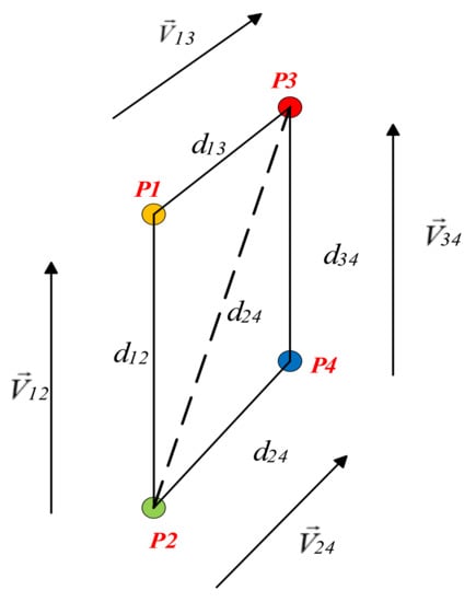
Figure 7. Diagram of feature geometric constraints.

The parallel vector constraint is shown in Figure 7, the expansion of mathematical expression of ${\stackrel{\rightharpoonup }{V}}_{12}||{\stackrel{\rightharpoonup }{V}}_{34}$ and ${\stackrel{\rightharpoonup }{V}}_{13}||{\stackrel{\rightharpoonup }{V}}_{24}$ in Cartesian coordinates is as follows:

$$\frac{p_{wx1}-p_{wx2}}{p_{wx3}-p_{wx4}}=\frac{p_{wy1}-p_{wy2}}{p_{wy3}-p_{wy4}}$$

(16)

$$\frac{p_{wx1}-p_{wx2}}{p_{wx3}-p_{wx4}}=\frac{p_{wz1}-p_{wz2}}{p_{wz3}-p_{wz4}}$$

(17)

$$\frac{p_{wy1}-p_{wy2}}{p_{wy3}-p_{wy4}}=\frac{p_{wz1}-p_{wz2}}{p_{wz3}-p_{wz4}}$$

(18)

$$\frac{p_{wx1}-p_{wx3}}{p_{wx2}-p_{wx4}}=\frac{p_{wy1}-p_{wy3}}{p_{wy2}-p_{wy4}}$$

(19)

$$\frac{p_{wx1}-p_{wx3}}{p_{wx2}-p_{wx4}}=\frac{p_{wz1}-p_{wz3}}{p_{wz2}-p_{wz4}}$$

(20)

$$\frac{p_{wy1}-p_{wy3}}{p_{wy2}-p_{wy4}}=\frac{p_{wz1}-p_{wz3}}{p_{wz2}-p_{wz4}}$$

(21)

The 12 equations contained in Equations (15) to (21) are geometric constraint equations with the unknown number as feature depth information $p_{wzi}$. Considering that there is four unknown depth information of four feature points, we need to reasonably select and use at least four of the 12 geometric constraint equations, so as to construct the multiple quadratic well-posed or overdetermined equation set $F$ about $p_{wzi}$, which can be obtained by solving $F$. Note that $p_{wzi}$ must be positive, and all non-positive solutions in the space of $F$ solution are pseudo-solutions.

It is particularly noteworthy that under our assumption if only the simplest case is considered, a scale constraint equation can be obtained for any two points of $n$ feature points in the space. Therefore, it can be realized as long as $C_n^2\ge n$ and $n\subseteq N$ is satisfied, that is, the minimum value of $n$ is 3. The reason why this algorithm uses the four-point method is to make full use of the parallel geometric constraints of the feature points in the space, which can greatly improve the estimation accuracy and robustness.

The rectangular target used in the experiment is only shown as a typical example. This method mainly discusses parallel features but is not limited to rectangles. For the case where a target is a plane, that is, the set of feature points acquired by vision are in the same plane, we can similarly use the multi-point coplanar constraint in the Cartesian coordinate system to replace the Equations (16) to (21). Additionally, using geometric constraints of feature point sets is more reliable and robust than simply using IMU assistance to obtain a motion baseline.

3.4. Improved Newton Iteration Method

The input of the improved Newton numerical iteration module is a set of depth equations constructed by projection equation and geometric constraints and the pose of UAV obtained by visual SLAM, and the output is the depth value of feature points and the final spatial position coordinates of the target. In this paper, an improved Newton–Raphson method with the fifth-order convergence is adopted, whose iterative equation is as follows:

$$Y^n=X^n-\frac{F\left(X^n\right)}{F^{\prime }\left(X^n\right)}$$

(22)

$$Z^n=X^n-\frac{2F\left(X^n\right)}{F^{\prime }\left(X^n\right)+F^{\prime }\left(Y^n\right)}$$

(23)

$$X^{n+1}=Z^n-\frac{F\left(Z^n\right)}{F^{\prime }\left(Y^n\right)}$$

(24)

where, $X^n$ is the vector to be solved composed of depth value $p_{wzi}$, $Y^n$ and $Z^n$ are the intermediate variables of the iteration. Considering the practical engineering application, the initial value of the unknown quantity in the algorithm vector $X^n$ is set to be 200, that is, the target feature point is assumed to be about 2 m in front of the UAV. In the actual test, it is found that the range of the initial value set from 0 to 800 has little effect on the accuracy and speed of the algorithm.

The termination conditions for our algorithm are as follows:

$$\Vert X^{n+1}-X^n\Vert {}_1<0.01\mathit{or}\eta \ge 20$$

(25)

where $\eta$ is the maximum number of iterations. By substituting the solved $p_{wzi}$ into Equation (14), the coordinates $P_{w}i$ of the spatial feature points of the target in the camera coordinate system can be obtained. R and T of the posture are obtained with the monocular VSLAM method:

$$R\cdot Pi+T=P_{w}i\Rightarrow Pi=R^{-1}\cdot P_{w}i-T$$

(26)

where $R$ is the rotation matrix of the camera relative to the world coordinate system, and T is the displacement vector of the camera relative to the world coordinate system. The coordinates $Pi$ of the target feature point in the world coordinate system can be obtained by solving the Equation (26).

Comparing the SPPM in this article with the traditional perspective-n-point (PnP) [49] method, it can be found that they have certain internal connections while there are also obvious differences between them. PnP method is to know the 3D position and 2D projection of a set of feature points to solve the camera’s pose. However, our problem assumes that the camera pose is known. The key problem of our research is to know the 2D projection of the feature points and the pose of the camera to solve the 3D position of the target. Our method utilizes the spatial scale constraints of projected feature points and the geometric constraints between feature points. Compared with the mainstream triangulation method using epipolar geometry and the currently popular method of using deep learning to obtain scale, SPPM has certain unique advantages. The following Table 1 shows the qualitative comparison between SPPF and the two mainstream depth estimation algorithms:

Table 1. Comparison of target depth positioning algorithms.

Method	Triangulation	Deep Learning	SPPM
Complexity	Medium	High	Low
Number of frames required	2 or more	Great amount	1
Required Information	Baseline	Template	Geometric Constraints
Required Sensor	Binocular or Mono-Inertial	Mono	Mono

In fact, since the scale of our target can be obtained at the same time when mono-SLAM is initialized, the subsequent algorithm of SPPM only needs a monocular sensor and one frame of image in each iteration. It can be seen that in scenes with parallel features or coplanar constraints, SPPM has the advantages of single-frame positioning and low complexity. It has a good spatial positioning ability for dynamic doors and windows with parallel features. Considering its characteristics for the use of parallel characteristics, ground static characteristics such as floor tiles and wooden floors are also suitable for this method.

3.5. Kalman Filter and Linear Regression

After the target position is obtained from the UAV vision, the center point of the door frame target is selected as the target point for tracking. Regarding the target movement as the uniform movement amount of the target point superimposed on the random movement amount, the random movement model of the target can be established. Assume that the state vector $S_k$ of the system includes the three-dimensional spatial position $x,y,z$ and the velocity $v_x,v_y,v_z$ at each moment $S_k={\left[\begin{array}{cccccc}x& v_x& y& v_y& z& v_z\end{array}\right]}^T$.

The Kalman filter equations are:

$$\stackrel{\wedge \_}{x_k}=A\stackrel{\wedge }{x_{k-1}}+D_{k-1}^{\prime }$$

(27)

$$P_k^{-}=A{P}_{k-1}{A}^T+Q$$

(28)

$$K_k=P_k^{-}{H}^T{(H{P}_k^{-}{H}^T+R)}^{-1}$$

(29)

$$\stackrel{\wedge }{x_k}=\stackrel{\wedge \_}{x_k}+K_k\left(z_k-H\stackrel{\wedge \_}{x_k}\right)$$

(30)

$$P_k=P_k^{-}-K_{k}H{P}_k^{-}$$

(31)

The system measurement equation is:

$$z_k=H\stackrel{\wedge }{x_k}+V_k$$

(32)

where $\stackrel{\wedge \_}{x_k}$ is the a priori state estimate value at the current moment k, $\stackrel{\wedge }{x_{k-1}}$ is the estimated value of the posterior state at k–1, $A$ is the state matrix of the system, $B$ is the matrix that converts the input to the state, $u_{k-1}$ is the control gain at k − 1, $P_k^{-}$ is the a priori estimated covariance at time k, $P_{k-1}$ is the posterior estimated covariance at k − 1 time, $Q$ is the process excitation noise covariance, $K_k$ is the Kalman filter gain matrix, $H$ is the conversion matrix from state variables to measurement, $R$ is the measurement noise covariance, and $z_k$ is the measured value. To extract information from the measured value more effectively, the various parameters of the filter are considered as follows:

• Under the condition of filter convergence, our method pays more attention to the convergence speed of the filter due to the rapid flight of the UAV. The original position of the measured value has little effect on the estimation. The initial value is determined as $S_k={\left[\begin{array}{cccccc}x& 0& y& 0& z& 0\end{array}\right]}^T$;
• For the process noise covariance matrix $Q$, since the random mobile interference $D_k$ in the state equation can be reflected by the measured value, $Q$ can take a small value;
• The measurement noise covariance $R$ is based on the actual measurement situation;
• Set the parameters of the filter, the initial covariance matrix $P_0=0.1E_6$, and the process noise covariance Matrix $Q=0.05E_6$, measurement noise covariance $R=0.5E_6$ ($E_n$ is the n-order identity matrix).

For dynamic targets such as the door frame which need to be crossed, we often need to predict the crossing position. Considering the instantaneity of flying through a door frame, linear regression fitting is made to a small segment of tracking data before the target image is lost to realize the estimation and prediction of the crossing point.

3.6. Flight Controller in Target Tracking

From the target space position, we can calculate the navigation coordinates required for UAV according to different tasks. For our platform, we introduce the PID controller for real-time flight control. The PID control method used in our system eliminates the need for a precise model of the system highly adaptive to various small quadrotors. In addition, it is robust to the changing controlled object and suited to industrial activities. The quadrotor adjusts its pose according to the positional deviation of the target and its own estimated position. The control law of the pitch angle and the yaw angle are given for examples as follows:

$$u_{\theta }=K_{p\theta }{e}_x+K_{d\theta }{\dot{e}}_x+K_{i\theta }\int e_{x}dt$$

(33)

$$e_x=X_t-X_e$$

(34)

$$u_{\psi }=K_{p\psi }{e}_{\psi }+K_{d\psi }{\dot{e}}_{\psi }$$

(35)

$$e_{\psi }={\psi }_t-{\psi }_e$$

(36)

where $u_{\theta }$ and $u_{\varphi }$ are control instructions of pitch angle and roll angle, $K_{p\theta }$, $K_{d\theta }$, and $K_{i\theta }$ are PID control gains, $X_t$ and $X_e$ are the target point and current estimated pose of x axis. Additionally, $u_{\psi }$ is yaw angle control instruction; $K_{p\psi }$ and $K_{d\psi }$ are PD control gains, ${\psi }_t$ and ${\psi }_e$ are the target point current estimated pose of yaw angle. By adjusting the control parameters, control signals can be set. PID control loop of AR.Drone2.0 is shown in Figure 8.

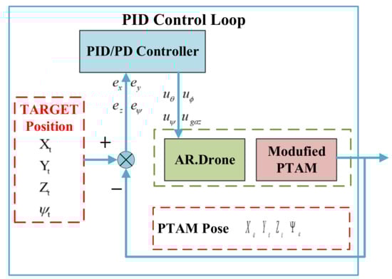
Figure 8. AR. Drone2.0 PID control loop.

4. Experimental Results and Analysis

4.1. Experimental Hardware Platform

A commercial UAV named AR.Drone2.0 made by Parrot, a French company, is used as the experimental verification platform. The UAV is equipped with a 200 Hz IMU, an ultrasonic altimeter, an air pressure sensor, and a set of 30 Hz dual cameras. The main characteristic parameters of AR.Drone2.0 are listed in Table 2 below. As the main sensor used in our system, the front-end camera covers a 92-diagonal field of view, with a maximum resolution of $1280\times 720$ at the refresh rate of 30 fps. The experimental platform meets the characteristics of monocular vision input required by our algorithm framework and features the advantages of high security and easy development. The core computing and processing platform used in the ground station is Lenovo Y410p with the i7-4700 processor.

Table 2. AR. DRONE2.0 characteristic parameters.

Parameters	Value
Size	45.2 cm × 45.2 cm
Weight	380 g
Maximum speed	18 km/h
Endurance	18 min
Operating radius	50 m

4.2. Transplantation of PTAM Module

The algorithm we transplanted to our UAV platform AR. Drone 2.0 is an improved PTAM proposed by Engel et al. [50] that effectively solved the scale uncertainty of the monocular camera. It applied to the self-posture estimation in our algorithm framework. Figure 9 shows the schematic diagram of the improved PTAM algorithm framework.

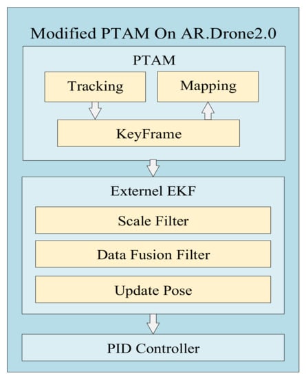
Figure 9. Modified PTAM used to estimate the pose.

4.3. Experimental Test Environment

In this paper, model analysis, static positioning test, dynamic flight verification, and other experiments were carried out under indoor conditions. In those experiments, a visual motion capture system named SVW4.V1 was employed to calibrate the true value of the target. The motion capture system (MCS) is composed of four cameras, which can cover the space experiment range of 3.5 m × 3.5 m × 3.5 m, and can achieve posture tracking and data recording with the refresh rate of 60 Hz. Figure 10 shows a panoramic view of the entire experimental scene.

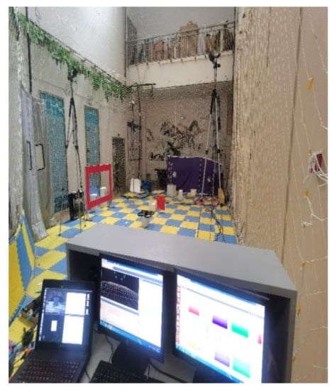
Figure 10. Experimental environment.

4.4. Laboratory Experiment and Result Analysis

4.4.1. Construction and Analysis of Geometric Constraint Equations

Experiment 1: The purpose of this experiment is to discuss and verify the reasonable construction of geometric constraint equations, analyze the usability of each group of geometric constraint equations, and analyze the time cost of the algorithm quantitatively for the three groups of available models.

In this experiment, the front-end ATAN camera of the UAV was used to detect with a fixed distance the four corners of the door frame target at a distance of 4 m. Different constraint models were constructed by the selection of different constraint equations, and the reliability and accuracy of the model under various conditions were analyzed. The long side of the door frame is 120.1 cm and the short side is 60 cm. The experimental results are shown in Table 3.

Table 3. Experimental results of the geometric constraint equations.

Method	Depth of Four Corners/cm				No.
Ground Truth	400	400	400	400	1
Newton Method	408	410	405	339	2
	0	0	0	0	3
	0	0	172	192	4
	*−	−	*+	+	5
	305	356	305	356	6
	352	389	405	393	7
	384	384	303	303	8
	399	393	399	396	9
	399	395	399	396	10
	402	404	403	397	11

*−: Negative value; *+: Positive value.

No. 1–11 represent different solution plans for constraint equations, in which No. 1 represents the real value of manual calibration, No. 2 represents the solution result of the original Newton method without using parallel constraint, and No. 3–11 represents the solution results of different constraint equations with improved Newton algorithm. Equations No. 3–12 are analyzed in Table 4.

Table 4. Analysis results of geometric constraint equations.

No.	Selection Mode	* NoE	Model Analysis
3	length of one long side + length of one short side + two equations for each opposite side parallel condition	4	Zero solution due to improper selection of parallel conditions
4	length of two diagonals + a set of two parallel conditions on opposite sides	4	Insufficient constraints for parallel conditions and diagonal lead to wrong solutions
5	length of two short sides + length of one diagonal +one parallel conditions on opposite sides	5	Insufficient constraints lead to negative spurious solutions
6	length of two short sides + a set of two parallel conditions on long opposite sides	4	Insufficient parallel conditions and diagonal constraints lead to wrong solutions
7	length of three sides + length of one diagonal	4	No use of parallel constraints leads to large solution error
8	length of two diagonals + a set of two parallel conditions on opposite sides	4	Insufficient constraints for diagonal and parallel condition leads to wrong solutions
9	length of four sides + a set of three parallel conditions on opposite sides	7	Redundant conditions, Overdetermined equations, Correct solutions
10	length of three sides + length of one diagonal + a set of three parallel conditions on opposite sides	7	Redundant conditions, Overdetermined equations, Correct solutions
11	length of two sides opposite sides + two parallel condition of the opposite sides	4	Reasonable constraints, Full rank equations, Correct solutions

* NoE: Number of Equations.

As shown in Table 3, the static mean square percentage error of equations No. 9 and No. 10 is less than 0.8% since redundant conditions are adopted, but high-precision depth solutions are obtained with strong constraint conditions and more calculation. Model No. 11 uses only four equations which are two opposite sides and the parallel condition of the opposite sides, and the static mean square error percentage is less than 0.75%. Model No. 11 is a good choice for solving depth information. Furthermore, the average time required by the two-dimensional target detection and the three-dimensional depth estimation for one image on the platform of general airborne computing unit NVIDIA Jetson TX2 of No. 9–11 models is presented, as shown in Table 5:

Table 5. Test of algorithmic efficiency on the airborne platform.

No.	Target Detection	Improve Newton Iteration
9	71.6 ms	2.93 ms
10	70.8 ms	2.76 ms
11	72.4 ms	1.81 ms

As seen in Table 5, the time consumption of the depth estimation used in this paper is short, which is far less than that of the two-dimensional target detection algorithm, and fully meets the real-time requirements in actual flight applications. The experiment shows that the depth solving equation system model No. 9–11 can achieve stable depth estimation. Additionally, the No. 11 model is characterized by advantages like a small amount of calculation and high precision.

4.4.2. Static Ranging Experiment and Analysis

Experiment 2: The purpose of this experiment is to quantitatively compare the accuracy and reliability of the original three-points Newton iteration method with the SPPM in this paper.

In this experiment, static ranging experiments were carried out for the center point of the square board target at three distances of 1 m, 1.5 m, and 2 m. The board is 34.8 cm long and 34.8 cm wide. In particular, we obtain the input images in a relatively dark environment which leads to an increase in a 2D detection error. The constraint equations of the SPPM used in the subsequent measurement in this paper are model No. 11. As a comparison, model No. 2, i.e., the original Newton numerical iteration, was used as the comparison experimental group under the same conditions. Figure 11 shows the comparison results of the manually calibrated real distance of the center point of the target, the improved Newton numerical iteration model (model No. 11), and the original Newton method (model No. 2).

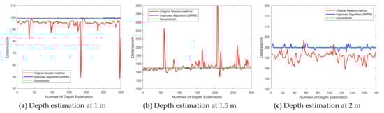
Figure 11. Results of Static measurement comparison.

Table 6 shows the root mean square error percentage (RMSPE) in this experiment:

Table 6. RMSPE of Experiment 2.

Distance	1 m	1.5 m	2 m
Original Newton method	8.01%	14.6%	1.62%
SPPM	1.03%	0.23%	0.31%

As shown in Figure 11 and Table 6, the original Newton iteration effect of the three-points method without using the parallel features can be very unstable while the quality of the input image is poor, which is easy to be affected by the detection noise. This experiment shows that static depth detection of the SPPM is stable and the detection accuracy is precise which meets the depth measurement needs of target features.

4.4.3. Experiment of Anti-Detection Error

Experiment 3: The purpose of this experiment is to quantitatively analyze the robustness of SPPM by manually adding random noise detection of feature points of the two-dimensional image.

In this experiment, the static anti-noise ability of the improved algorithm is discussed. Similarly, three distances of 1 m, 1.5 m, and 2 m were detected in this experiment. In one group of the codes of the target detection module, random detection noise with the range within three pixels were manually added to analyze the anti-noise ability of the SPPM. Figure 12 shows the comparison diagram of static ranging.

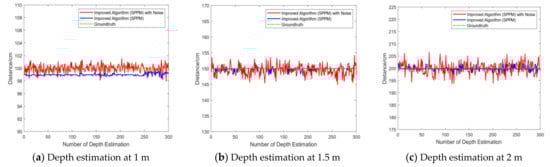
Figure 12. Results of static anti-noise comparison.

Table 7 shows the root mean square error percentage in this experiment:

Table 7. RMSPE of Experiment 3.

Distance	1 m	1.5 m	2 m
RMSPE	1.04%	0.23%	0.34%

As shown in Figure 12 and Table 7, the numerical iterative detection algorithm possesses good anti-noise ability. Even if the random detection noise is artificially added, the RMSPE value will not increase significantly, and it will remain within a reasonable range of 1.10%. In practical engineering applications, the detection algorithm often cannot guarantee absolute accuracy, so good anti-noise ability is of great significance for UAV target tracking. This experiment verifies that SPPM has excellent anti-noise ability, which greatly improves the robustness of target positioning under the condition of image detection noise in the actual flight mission of the UAV. It is worth noting that at 1 m, the error is larger than other positions. After data analysis, we believe that the main reason is that the true value of our manual measurement has a slight deviation during the test at 1 m. This may cause an impact on the calculation of RMSPE. However, in multiple experiments, the RMSPE is almost less than 1%, which verifies the reliability and stability of the method.

4.4.4. Flight Experiment and Analysis of Dynamic Target Tracking

Experiment 4: The purpose of this experiment is to comprehensively verify the effectiveness, stability, and accuracy of SPPM for moving target tracking.

This experiment is used to verify the target tracking ability of the algorithm in the actual flight mission. The tracking target is the square board in the previous static test. In this experiment, the UAV would continuously track the target. The following mode was to keep flying at 1.5 m forward of the normal of the center point of the board. The real trajectories of the target and the aircraft were provided by the motion capture system SVW4.V1. Figure 13 shows the trajectories of the aircraft in the tracking state when the target is hovering. The red line shows the flight path when the improved algorithm is used, the blue line shows the flight path with the original Newton iterative algorithm, and the green dot represents the hovering point of the aircraft in theory.

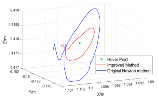
Figure 13. Static target tracking experiment.

The three-dimensional root mean square error of the improved algorithm is less than 2.8 cm, and the root mean square error of the original Newton iteration is about 4.5 cm. However, it is worth noting that in the 10 flight experiments, the original Newton iteration method has failed in 4 times, while stable tracking is achieved in all the ten times by using SPPM.

Figure 14 shows the estimated trajectory of the UAV and the actual trajectory of the small board when a small board target is used as the dynamic target.

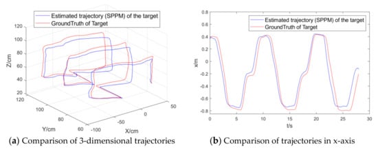
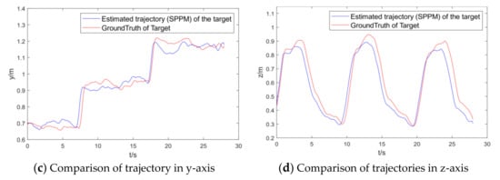
Figure 14. UAV dynamic target tracking result.

Table 8 shows the root mean square error of dynamic target tracking in this flight experiment.

Table 8. RMSE of dynamic target tracking.

Axis	X	Y	Z
RMSE	8.24 cm	3.43 cm	5.12 cm

Figure 15 shows the comparison between the estimated positioning trajectory of the UAV itself and the actual motion trajectory obtained by the motion capture system in the case of dynamic target tracking.

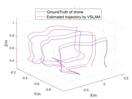
Figure 15. PTAM positioning experiment.

Table 9 shows the root mean square error in the UAV PTAM positioning experiment.

Table 9. RMSE of PTAM Positioning.

Axis	X	Y	Z
RMSE	7.92 cm	3.12 cm	5.48 cm

As shown by the data in Figure 14 and Table 8, the visual target tracking algorithm framework in this paper can well realize the dynamic detection and tracking of the indoor semi-cooperative target with the actual accuracy of centimeter-level by using parallel constraint, which is able to implement the visual tracking of the dynamic target.

As indicated by the data in Figure 15 and Table 9, the actual accuracy of the improved PTAM visual positioning algorithm also reaches the centimeter level. It can be obtained from this experiment that the moving target positioning and tracking algorithm of this paper meets the requirements of autonomous positioning and target positioning tracking accuracy required by most practical indoor flight applications.

4.4.5. Flying through a Door Frame

Experiment 5: The purpose of this experiment is to comprehensively verify the reliability and stability of the algorithm in applications like more complex target tracking, obstacle avoidance, and target trajectory.

Considering that obstacle avoidance and crossing are very common in indoor applications of the UAV, the experiments of autonomous identification, tracking, and flying through a dynamic door frame of the UAV were realized with the help of a moving door frame. Considering that the UAV cannot attain complete target image information before approaching the target and the instantaneity of the UAV flying through the door frame, the method was to sample and linearly fit the door frame motion in a short time, with 100 sampling points, which took about 3 s to realize the motion estimation. Figure 16 shows the sequence diagram group of flying through the door frame and Figure 17 shows the trajectory movement of the UAV and the center point of the door frame in the direction of Y-axis:

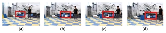
Figure 16. Flying through the dynamic door frame: figures (a–d) show the sequence diagram of the drone flying through a moving door frame.

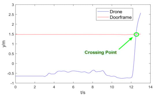
Figure 17. Trajectory of door crossing in the Y axis.

As shown in Figure 17, the position marked by the green ellipse is the actual door frame crossing point of the drone. In this experiment, the trajectory tracking and estimation method used by the algorithm can use the sampling information before the near flying through a door frame to successfully estimate a reasonable crossing point and quickly complete the crossing task.

5. Conclusions

An efficient dynamic target positioning solution, namely SPPM, is proposed in this paper for small quadrotor UAVs using a monocular vision sensor. The key idea of SPPM is to model the geometric constraint equations of the feature points of the moving target, and improve the depth estimation accuracy and robustness by an improved Newton numeric iteration algorithm. Based on SPPM, a UAV visual positioning and tracking framework that integrates target feature recognition, monocular SLAM positioning, and dynamic target tracking is designed.

Indoor flight experiments have verified: (1) The static tracking error of SPPM is less than 1.03% and it has good robustness in the presence of detection errors. (2) The RMSE of SPPM for hovering and tracking a static target is less than 2.8 cm. (3) The RMSE of SPPM tracking random moving targets is less than 7.92 cm and it has good capabilities of stability and long-term tracking.

Future research directions include the following aspects: (1) Extend the solution developed in this paper to the task scenes where multiple UAVs are required to fly through the moving door frames in a coordinated manner. The difficulty of this problem lies in the multi-view image information fusion and multi-UAVs real-time communication. (2) The approaches to model other geometric constraints with different types of features will be studied (such as linear constraints, spherical constraints) to improve the adaptivity to the moving obstacles of other shapes.

References

- Weiss, S.; Achtelik, M.W.; Lynen, S.; Chli, M.; Siegward, R. Real-time onboard visual-inertial state estimation and self-calibration of mavs in unknown environments. In Proceedings of the 2012 IEEE International Conference on Robotics and Automation, Saint Paul, MN, USA, 14–18 May 2012; pp. 957–964. [Google Scholar]
- Chowdhary, G.; Johnson, E.N.; Magree, D.; Wu, A.; Shein, A. GPS-denied Indoor and Outdoor Monocular Vision Aided Navigation and Control of Unmanned Aircraft. J. Field Robot. 2013, 30, 415–438. [Google Scholar] [CrossRef]
- Ruan, W.-Y.; Duan, H.-B. Multi-UAV obstacle avoidance control via multi-objective social learning pigeon-inspired optimization. Front. Inf. Technol. Electron. Eng. 2020, 21, 740–748. [Google Scholar] [CrossRef]
- Shao, Y.; Zhao, Z.-F.; Li, R.-P.; Zhou, Y.-G. Target detection for multi-UAVs via digital pheromones and navigation algorithm in unknown environments. Front. Inf. Technol. Electron. Eng. 2020, 21, 796–808. [Google Scholar] [CrossRef]
- Yang, T.; Li, P.; Zhang, H.; Li, J.; Li, Z. Monocular Vision SLAM-Based UAV Autonomous Landing in Emergencies and Unknown Environments. Electronics 2018, 7, 73. [Google Scholar] [CrossRef] [Green Version]
- Mahony, R.; Kumar, V.; Corke, P. Multirotor Aerial Vehicles: Modeling, Estimation, and Control of Quadrotor. IEEE Robot. Autom. Mag. 2012, 19, 20–32. [Google Scholar] [CrossRef]
- Shen, S.; Michael, N.; Kumar, V. Autonomous indoor 3D exploration with a micro-aerial vehicle. In Proceedings of the 2012 IEEE International Conference on Robotics and Automation, Saint Paul, MN, USA, 14–18 May 2012; pp. 9–15. [Google Scholar]
- Orgeira-Crespo, P.; Ulloa, C.; Rey-Gonzalez, G.; García, J.P. Methodology for Indoor Positioning and Landing of an Unmanned Aerial Vehicle in a Smart Manufacturing Plant for Light Part Delivery. Electronics 2020, 9, 1680. [Google Scholar] [CrossRef]
- Akhtar, N.; Mian, A. Threat of Adversarial Attacks on Deep Learning in Computer Vision: A Survey. IEEE Access 2018, 6, 14410–14430. [Google Scholar] [CrossRef]
- Yuan, X.; Feng, Z.-Y.; Xu, W.-J.; Wei, Z.-Q.; Liu, R.-P. Secure connectivity analysis in unmanned aerial vehicle networks. Front. Inf. Technol. Electron. Eng. 2018, 19, 409–422. [Google Scholar] [CrossRef]
- Lu, Y.; Xue, Z.; Xia, G.-S.; Zhang, L. A survey on vision-based UAV navigation. Geo-Spat. Inf. Sci. 2018, 21, 21–32. [Google Scholar] [CrossRef] [Green Version]
- Zhu, X.; Zhang, X.; Qu, Y. Consensus-based three-dimensional multi-UAV formation control strategy with high precision. Front. Inf. Technol. Electron. Eng. 2017, 18, 968–977. [Google Scholar]
- Falanga, D.; Mueggler, E.; Faessler, M.; Scaramuzza, D. Aggressive quadrotor flight through narrow gaps with onboard sensing and computing using active vision. In Proceedings of the 2017 IEEE International Conference on Robotics and Automation (ICRA), Singapore, 29 May–3 June 2017; pp. 5774–5781. [Google Scholar] [CrossRef] [Green Version]
- Pachauri, A.; More, V.; Gaidhani, P.; Gupta, N. Autonomous Ingress of a UAV through a window using Monocular Vision. arXiv 2016, arXiv:1607.07006. [Google Scholar]
- Zhao, F.; Zeng, Y.; Wang, G.; Bai, J.; Xu, B. A Brain-Inspired Decision Making Model Based on Top-Down Biasing of Prefrontal Cortex to Basal Ganglia and Its Application in Autonomous UAV Explorations. Cogn. Comput. 2017, 10, 296–306. [Google Scholar] [CrossRef]
- Albrektsen, S.M.; Bryne, T.H.; Johansen, T.A. Robust and secure UAV navigation using GNSS, phased-array radio system and inertial sensor fusion. In Proceedings of the 2018 IEEE Conference on Control Technology and Applications (CCTA), Copenhagen, Denmark, 21–24 August 2018; pp. 1338–1345. [Google Scholar]
- Weiss, U.; Biber, P. Plant detection and mapping for agricultural robots using a 3D LIDAR sensor. Robot. Auton. Syst. 2011, 59, 265–273. [Google Scholar] [CrossRef]
- Henry, P.; Krainin, M.; Herbst, E.; Ren, X.; Fox, D. RGB-D mapping: Using Kinect-style depth cameras for dense 3D modeling of indoor environments. Int. J. Robot. Res. 2012, 31, 647–663. [Google Scholar] [CrossRef] [Green Version]
- Triggs, B.; McLauchlan, P.F.; Hartley, R.I.; Fitzgibbon, A.W. Bundle adjustment—A modern synthesis. In Vision Algorithms: Theory and Practice, Proceedings of the International Workshop on Vision Algorithms, Corfu, Greece, 21–22 September 1999; Springer: Berlin/Heidelberg, Germany, 1999; pp. 298–372. [Google Scholar]
- Wang, Y.; Wang, P.; Yang, Z.; Luo, C.; Yang, Y.; Xu, W. UnOS: Unified unsupervised optical-flow and stereo-depth estimation by watching videos. In Proceedings of the IEEE/CVF Conference on Computer Vision and Pattern Recognition (CVPR), Long Beach, CA, USA, 9 January 2020; pp. 8063–8073. [Google Scholar] [CrossRef]
- Cheng, H.; An, P.; Zhang, Z. Model of relationship among views number, stereo resolution and max stereo angle for multi-view acquisition/stereo display system. In Proceedings of the 9th International Forum on Digital TV and Wireless Multimedia Communication, IFTC 2012, Shanghai, China, 9–10 November 2012; pp. 508–514. [Google Scholar] [CrossRef]
- Gomez-Ojeda, R.; Moreno, F.-A.; Zuniga-Noel, D.; Scaramuzza, D.; Gonzalez-Jimenez, J. PL-SLAM: A Stereo SLAM System Through the Combination of Points and Line Segments. IEEE Trans. Robot. 2019, 35, 734–746. [Google Scholar] [CrossRef] [Green Version]
- Qin, T.; Li, P.; Shen, S. Relocalization, global optimization and map merging for monocular visual-inertial SLAM. In Proceedings of the 2018 IEEE International Conference on Robotics and Automation (ICRA), Brisbane, Australia, 21–25 May 2018; pp. 1197–1204. [Google Scholar]
- Weiss, S.; Achtelik, M.W.; Lynen, S.; Achtelik, M.C.; Kneip, L.; Chli, M.; Siegwart, R. Monocular Vision for Long-term Micro Aerial Vehicle State Estimation: A Compendium. J. Field Robot. 2013, 30, 803–831. [Google Scholar] [CrossRef]
- Qin, T.; Li, P.; Shen, S. VINS-Mono: A Robust and Versatile Monocular Visual-Inertial State Estimator. IEEE Trans. Robot. 2018, 34, 1004–1020. [Google Scholar] [CrossRef] [Green Version]
- Nützi, G.; Weiss, S.; Scaramuzza, D.; Siegwart, R. Fusion of IMU and vision for absolute scale estimation in monocular SLAM. J. Intell. Robot. Syst. 2010, 61, 287–299. [Google Scholar] [CrossRef] [Green Version]
- Zhou, D.; Dai, Y.; Li, H. Ground-Plane-Based Absolute Scale Estimation for Monocular Visual Odometry. IEEE Trans. Intell. Transp. Syst. 2019, 21, 791–802. [Google Scholar] [CrossRef]
- Qiu, K.; Liu, T.; Shen, S. Model-Based Global Localization for Aerial Robots Using Edge Alignment. IEEE Robot. Autom. Lett. 2017, 2, 1256–1263. [Google Scholar] [CrossRef]
- Gan, Y.; Xu, X.; Sun, W.; Lin, L. Monocular depth estimation with affinity, vertical pooling, and label enhancement. In Proceedings of the European Conference on Computer Vision (ECCV), Munich, Germany, 8–14 September 2018; pp. 224–239. [Google Scholar]
- Zou, Y.; Luo, Z.; Huang, J.-B. DF-Net: Unsupervised joint learning of depth and flow using cross-task consistency. In Proceedings of the European Conference on Computer Vision (ECCV), Munich, Germany, 8–14 September 2018; pp. 38–55. [Google Scholar] [CrossRef] [Green Version]
- Bendig, J.; Bolten, A.; Bareth, G. Introducing a low-cost mini-UAV for thermal- and multispectral-imaging. Int. Arch. Photogramm. Remote Sens. Spat. Inf. Sci. 2012, XXXIX-B1, 345–349. [Google Scholar] [CrossRef] [Green Version]
- Wang, Z.H.; Zhang, T.; Qin, K.Y.; Zhu, B. A Vision-Aided Navigation System by Ground-Aerial Vehicle Cooperation for UAV in GNSS-Denied Environments. In Proceedings of the 2018 IEEE CSAA Guidance, Navigation and Control Conference (CGNCC), Xiamen, China, 10–12 August 2018; pp. 1–6. [Google Scholar]
- Wang, N.; Wang, G.Y. Shape Descriptor with Morphology Method for Color-based Tracking. Int. J. Autom. Comput. 2007, 4, 101–108. [Google Scholar] [CrossRef]
- Tsai, D.M.; Molina, D.E.R. Morphology-based defect detection in machined surfaces with circular tool-mark patterns. Measurement 2019, 134, 209–217. [Google Scholar] [CrossRef]
- Yin, J.; Fu, C.; Hu, J. Using incremental subspace and contour template for object tracking. J. Netw. Comput. Appl. 2012, 35, 1740–1748. [Google Scholar] [CrossRef]
- Guo, J.; Zhu, C. Dynamic displacement measurement of large-scale structures based on the Lucas–Kanade template tracking algorithm. Mech. Syst. Signal. Process. 2016, 66–67, 425–436. [Google Scholar] [CrossRef]
- Henriques, J.F.; Caseiro, R.; Martins, P.; Batista, J. High-Speed Tracking with Kernelized Correlation Filters. IEEE Trans. Pattern Anal. Mach. Intell. 2015, 37, 583–596. [Google Scholar] [CrossRef] [Green Version]
- Li, H.; Shen, C.; Shi, Q. Robust real-time visual tracking with compressed sensing. In Proceedings of the CVPR 2011, Colorado Springs, CO, USA, 20–25 June 2011; pp. 1305–1312. [Google Scholar]
- Kumar, N.; Parate, P. Fragment-based real-time object tracking: A sparse representation approach. In Proceedings of the 2012 19th IEEE International Conference on Image Processing, Orlando, FL, USA, 30 September–3 October 2012; pp. 433–436. [Google Scholar]
- Qin, Y.; Shen, G.; Zhao, W.; Che, Y.; Yu, M.; Jin, X. A network security entity recognition method based on feature template and CNN-BiLSTM-CRF. Front. Inf. Technol. Electron. Eng. 2019, 20, 872–884. [Google Scholar] [CrossRef]
- Pang, S.; del Coz, J.J.; Yu, Z.; Luaces-Rodriguez, O.; Diez-Pelaez, J. Deep learning to frame objects for visual target tracking. Eng. Appl. Artif. Intell. 2017, 65, 406–420. [Google Scholar] [CrossRef] [Green Version]
- Devernay, F.; Faugeras, O. Straight lines have to be straight. Mach. Vis. Appl. 2001, 13, 14–24. [Google Scholar] [CrossRef]
- Noor, M.A.; Waseem, M. Some iterative methods for solving a system of nonlinear equations. Comput. Math. Appl. 2009, 57, 101–106. [Google Scholar] [CrossRef] [Green Version]
- Kou, J.; Li, Y.; Wang, X. Some modifications of Newton’s method with fifth-order convergence. J. Comput. Appl. Math. 2007, 209, 146–152. [Google Scholar] [CrossRef] [Green Version]
- Sharma, J.R.; Gupta, P. An efficient fifth order method for solving systems of nonlinear equations. Comput. Math. Appl. 2014, 67, 591–601. [Google Scholar] [CrossRef]
- Zhou, W.; Hou, J. A New Adaptive Robust Unscented Kalman Filter for Improving the Accuracy of Target Tracking. IEEE Access 2019, 7, 77476–77489. [Google Scholar] [CrossRef]
- Al-Kanan, H.; Li, F. A Simplified Accuracy Enhancement to the Saleh AM/AM Modeling and Linearization of Solid-State RF Power Amplifiers. Electronics 2020, 9, 1806. [Google Scholar] [CrossRef]
- Chum, O. Two-View Geometry Estimation by Random Sample and Consensus. Ph.D. Thesis, CTU, Prague, Czech Republic, 2005. [Google Scholar]
- Gao, X.S.; Hou, X.R.; Tang, J.; Cheng, H.-F. Complete solution classification for the perspective-three-point problem. IEEE Trans. Pattern Anal. Mach. Intell. 2003, 25, 930–943. [Google Scholar]
- Engel, J.; Sturm, J.; Cremers, D. Scale-aware navigation of a low-cost quadrocopter with a monocular camera. Robot. Auton. Syst. 2014, 62, 1646–1656. [Google Scholar] [CrossRef] [Green Version]
Publisher’s Note: MDPI stays neutral with regard to jurisdictional claims in published maps and institutional affiliations. |
© 2021 by the authors. Licensee MDPI, Basel, Switzerland. This article is an open access article distributed under the terms and conditions of the Creative Commons Attribution (CC BY) license (https://creativecommons.org/licenses/by/4.0/).