Abstract
In recent times, particulate matter (PM2.5) is one of the most critical air quality contaminants, and the rise of its concentration will intensify the hazard of cleanrooms. The forecasting of the concentration of PM2.5 has great importance to improve the safety of the highly pollutant-sensitive electronic circuits in the factories, especially inside semiconductor industries. In this paper, a Single-Dense Layer Bidirectional Long Short-term Memory (BiLSTM) model is developed to forecast the PM2.5 concentrations in the indoor environment by using the time series data. The real-time data samples of PM2.5 concentrations were obtained by using an industrial-grade sensor based on edge computing. The proposed model provided the best results comparing with the other existing models in terms of mean absolute error, mean square error, root mean square error, and mean absolute percentage error. These results show that the low error of forecasting PM2.5 concentration in a cleanroom in a semiconductor factory using the proposed Single-Dense Layer BiLSTM method is considerably high.
1. Introduction
In the last few years, many attempts have been made to create the system architecture of a smart factory. The Industrial Internet of Things (IIoT) has recently been implemented as an integration of the Internet of Things in the manufacturing or industrial fields. With the assistance of a cyber-physical system (CPS), the industrial sector has undertaken a new paradigm shift regarding physical device or tool control level up to the higher levels of the business process management systems as a key component of industrial 4.0 systems [1]. CPS refers to smart machines, storage systems, and production facilities that are capable of autonomously sharing information, triggering actions, and controlling one another [2].
In terms of a smart factory, continuous monitoring of air quality is needed to protect production outputs (i.e., semiconductors from damage caused by air pollution) and a system is needed that can accurately predict future air quality by forecasting particulate matter (PM). Different types of contaminants are distributed in the air depending on human and environmental factors. One of the most critical among all the pollutants is PM2.5 (fine inhalable particles, with an aerodynamic diameter that is commonly 2.5 micrometers or smaller) [3], potentially creating a big problem for the smart factory field. In addition, these particles may cause the deformity of semiconductor chips [4], resulting in wafer defects which would reduce profit and increases the maintenance cost [5], especially in the semiconductor industry. Defects of semiconductor chips or wafers can be caused by airborne particulates as small as 1µm. In order to minimize the concentration of particulates in the air, special precautions are needed to be undertaken during the processing of semiconductors [6]. This is because of the high potential damage caused by particulate matter in the cleanroom of semiconductor factories, for which the forecasting of PM2.5 concentration is critical for predictive maintenance. Moreover, this method is very important for factories’ allocation of resources for planning, preparation, and preventive actions for any potential damage caused by particulates.
A variety of methods have been developed to predict PM2.5 concentration by using the time series data. Therefore, these existing approaches include machine learning (ML) and deep learning (DL) methods. Moreover, several forecasting models have been widely implemented in recurrent neural networks (RNNs) [7] and their derivations [8], such as long short-term memory (LSTM) [9], a convolutional neural network long short-term memory (CNN-LSTM) [10], and Transformer [11]. Athira et al. [7] had predicted PM2.5 by using RNN to be compared with the gated recurrent unit. Chen et al. [8] used RNN and its derivatives to predict PM2.5, but the results need to be improved in accuracy and compared with other artificial intelligence methods. However, there are problems found in RNN models: training an RNN is a difficult task, involving gradient vanishing and exploding [11], and it cannot proceed with very long sequences if tanh or ReLU are used as activation functions. Xayasouk et al. [9] used LSTM and deep autoencoder models to predict fine particulate matter, but their result required the development of an alternative design of deep learning models to gain more accurate output. Li et al. [10] used hybrid CNN-LSTM to forecast PM2.5 but did not compare their method to other deep learning models. In addition, the Transformer method [11], which is commonly used for natural language processing (NLP), was also used to predict data based on time series data, but the authors did not discuss the detailed mechanism of their proposed model. In this work, we developed a new proposed model by considering the dense layer and comparing its results with other deep learning methods. To achieve the best outputs, we developed, implemented, and enhanced a time series predicting approach based on a bidirectional long-short-term-memory (BiLSTM) artificial neural network (ANN) architecture [7]. A BiLSTM is a sequence processing model made up of two LSTMs, one of which takes the input in one direction, and the other in the opposite direction. In this paper, forecasting PM2.5 was used as a case study to show that a single-dense BiLSTM model can be successfully applied to the task of predicting times series data, and it outperforms many existing predicting techniques.
Specifically, our contributions are the following:
- To get reliable data, we employed hardware architecture based on edge computing to meet compatibility with the IIoT system.
- Using PM2.5 forecasting as a case study, we demonstrate that our Single-Dense Layer BiLSTM model can accurately forecast PM2.5 concentration.
- Our contribution centered on developing a system that provides computationally efficient, potent, and stable performance with a small number of parameters.
- Our findings show that compared with the LSTM, CNN-LSTM, and Transformer methods, the Single-Dense Layer BiLSTM achieves the lowest error.
The remainder of this paper is organized as follows: Section 2 describes the proposed system related to the phases of the research from data sensing until DL-based services. Section 3 provides the methodology of the proposed model, which is compared with other DL models. Section 4 explains the forecasted data using the Single-Dense Layer BiLSTM model and compares it with other DL models with various hyperparameters, then analyzes the forecasted data with high similarity to the real data. Conclusions for the forecasting using the Single-Dense Layer BiLSTM model are presented in Section 5.
2. System Overview
Figure 1 shows the overall architecture of the system. In the proposed system, the industrial-grade sensor is deployed in a laboratory clean room. The PM2.5 data is collected from the industrial-grade sensor and then stored in the edge database. The data is collected for a single day which contains 86,400 pieces of PM2.5 data. The data collection took place in an indoor environment during the spring season in April 2021 in the engineering laboratory of Kookmin University. The personal computer (PC) that used in this study is Windows 10 Pro for Workstations, RAM 256 GB, Intel® Xeon® Gold 5222 CPU @3.80GHz 3.79 GHz and 64-bit Operating System, x64-based processor. The proposed system comprises three-phase processes consisting of data sensing, a knowledge discovery in database (KDD), and deep learning (DL)-based services.
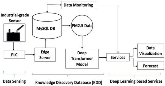
Figure 1.
The hardware architecture with three phases of the proposed data acquisition system: data sensing, KDD, and deep learning-based services.
In the phase of data sensing, to set this research to be compatible with the IIoT system in a semiconductor factory, the industrial-grade sensor is used to collect PM2.5 data. The sensor is installed with RS485 and connected to a programmable logic controller (PLC) to enable various communication methods, making it a perfect data acquisition and control system for a wide range of applications [12]. Thus, the data can be read by the server in a real-time mode.
In this phase, the data collection process consists of acquiring and selecting raw data from the sensor, which contains temperature, humidity, PM1, and PM2.5. These were collecting and selecting raw data tasks managed by the edge server using IEC 61131-3 standard, which is run on PLCs. The IEC 61131-3 standard is a widely accepted international standard for PLCs and specifies five programming languages: LD, FBD, Instruction List (IL), SFC, and ST [13]. The ST programming language is used in this research. ST is a text-based, high-level programming language that allows the user to create complex algorithms in the applications. As a result, it is often to be used to develop a large-scale PLC system.
In the second phase, the edge computing-based KDD process is used to define the technique widely to identify and interpret patterns in data that can be used to construct or forecast future events [14]. We optimize the edge computing technology that could move the network, computing power, storage, and resources of the cloud to the edge of the network. Edge computing could also provide intelligent services at the edge to meet the critical industry needs of real-time business, data optimization, application intelligence, security, and privacy and satisfy the network demand for low latency and high bandwidth. The edge computing downlink data acts as a cloud service, the uplink data indicates the Internet of Everything (IoE), and the edge computing allocates any computing and network systems between the data source and the path of the cloud computing center [15]. In this work, edge computing data from the data collection phase was processed before it was stored in the MySQL database.
As shown in Figure 1, KDD is an iterative method for converting raw data into usable data [16]. The data from the edge server is stored in the MySQL database application. MySQL, like other relational systems, stores data in tables and accesses databases using SQL. In MySQL, the user can set up rules to regulate the relationships between the fields in the tables and pre-defined user database schema according to their needs. The Oracle Corporation developed, distributed, and supported MySQL, a popular open-source relational database management system (RDBMS) [17].
To get clean PM2.5 concentration data as the input to the Single-Dense Layer BiLSTM method, the data preprocessing involves extracting features from the raw data. It also includes the application of cleaning methods to avoid problem data such as missing values. The cleaning application also removes the involvement of new features.
Once PM2.5 data as output from data preprocessing was collected, the next step was data mining, which is the core of the KDD process. It comprises selecting and applying techniques, including implementing DL models. Data mining also could extract features from data by finding applied patterns and relations between features. The type of DL algorithm is determined by the problem at hand and the quality of the data available. The efficiency and effectiveness of the data mining algorithm of the tasks, as a result, carried out in previous steps of the KDD method, are measured using a collection of metrics during interpretation and evaluation. After that, the processed data was used in the Single-Dense Layer BiLSTM model to predict particle concentration.
The last phase of our proposed architecture is DL-based services. In this phase, we used Jupyter Notebook to run our experiments and visualize the results. The Jupyter Notebook is built on a collection of open standards for collaborative computing. These open standards can be used by third-party developers to build personalized applications with embedded interactive computing [18]. Other benefits of Jupyter Notebook are allowing seamless integration of code, narrative text, and figures into a single live executable and editable document [19].
3. Methodology
3.1. Data Preprocessing
Deep learning is one of the fundamental approaches in machine learning, and it is used for forecasting and other applications. Here, we discuss the Single-Dense Layer BiLSTM as one of the deep learning methods that we have used in this research to perform the forecasting task. Data preprocessing in Single-Dense Layer BiLSTM is essential to clean the data and make it applicable for the deep learning model and improve the accuracy and efficiency of the model. Data cleaning and normalization are two steps in the process of data processing. Data cleaning involves deleting anomalous values from the data set and filling in blanks. To overcome this issue, we fill NaN values by using the interpolation method. The NaN, which stands for “not a number”, denotes any undefined or unpresentable value [20]. The linear method was selected in this interpolate method, handling the values as evenly distributed [21]. Moreover, in terms of mean square error (MSE), using a linear method for interpolation is better than the last observation carried forward (LOCF) and the next observation carried backward (NOCB) because the linear method has the lowest MSE value compared with LOCF and NOCB [22].
Normalizing the data can speed up the convergence rate of the gradient descent and increase the performance of the predictive model. When dealing with non-standardized data, gradient descent can become quite arduous [23]. Normalization also makes it uncomplicated for deep learning models to extract extended features from numerous historical output data sets, potentially improving the performance of the proposed model. In this study, after collection of the bulk historical data, we normalized the PM 2.5 values to trade-off between prediction accuracy and training time using the Min-Max normalization method given in Equation (1):
where is the original data, is the normalized value, and , represent maximum and minimum data points in the time series data sample, respectively. Now, we have converted unsupervised time series data into a supervised format for each case of prediction, namely, 5 min ahead prediction, 30 min ahead prediction, and 1 h ahead prediction. The formation of supervised time series data is very crucial. The formations of input matrices and corresponding output matrices are given below:
For 5 min ahead prediction:
For 30 min ahead prediction:
For 1 h ahead prediction:
Meanwhile, we employed a train/validation/test (64%/16%/20%) approach to consider PM2.5 concentration as time-series data [10]. Before we describe the actual framework of the model, we will discuss some valuable time-series forecasting models which are important methods to be compared to our proposed model.
3.2. RNN Model
RNNs, unlike feedforward neural networks, can process sequences of inputs using their internal state (memory). In the RNN, all the inputs are linked together. Neural networks improve performance in a variety of engineering applications, such as prediction [24] and human behavior modeling [25], among neural networks. Specifically, RNNs are implemented to model temporal and time-series data due to having built-in memory retaining past information [26]. By adding feedback connections, the RNN is elongated from the feedforward neural network to the model sequence knowledge. Specifically, given (x1, x2, …, xn) as the input sequence, the standard RNN can gain another sequence (y1, y2, …, yn) iteratively by the following equations:
where h is the hidden state, φ (·) expresses the activation functions, W, U, b are the weights and biases to be learned, respectively [27]. The simple RNNs need control structures because the norm of gradient deteriorated in a fast manner amid training, i.e., during the exploding and vanishing gradient problems. As a result, the simple RNNs are inadequate to capture long-term and short-term dependencies [28]. To solve this problem, the long short-term memory (LSTM) network, a novel RNN architecture with control structures, as shown in Figure 2, is implemented [29]. As depicted in Figure 2, the yellow circles illustrate the hidden states that stand for Yt, where t is the time step. “R” is the recurrent unit that collects input Xt and output Yt.
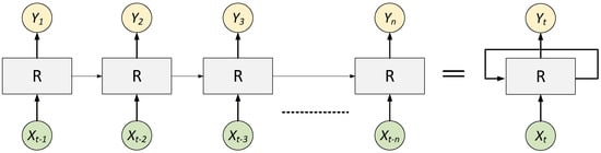
Figure 2.
RNN architecture.
3.3. LSTM Model
LSTM networks are an advanced version of RNNs that makes it easier to remember past knowledge. The vanishing gradient problem of the RNN is solved in this method. LSTM is well suited for identifying, processing, and forecasting a time series of unknown length time lags. The model is trained using back-propagation. In an LSTM network, there are three gates. Since LSTM networks have additional nonlinear control structures with multiple parameters, training issues can arise. Highly effective and efficient training methods for the LSTM architecture are implemented to address these issues [30].
An LSTM architecture with many memory cells is shown in Figure 3.
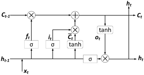
Figure 3.
LSTM architecture.
These memory cells are used to retain long-term time dependencies by storing past historical data. An LSTM is a set of units with the same parameters at all time steps. The LSTM model contains three memory cells: input, forget, and output gates, denoted as , , , respectively. The learning process updates these gates to train datasets. We first introduce how to update functions of LSTM:
where σ represents an element-wise sigmoid function with value in (0,1); φ represents an element-wise tanh function and is the Hadamard (element-wise) product; Wi, Wc, Wf, and Wo represent the correlation weight matrices for input x and input node it, input gate ct, forget gate , and output gate , respectively. Then, bi, bc, bf, and bo are biases of the input node it, input gate ct, forget gate , and output gate ; stands for element-wise multiplication, and represents element-wise hyperbolic tangent linear activation function [31]. Vectors b ∈ R and H are constant parameters where H refers to the number of hidden units. For each hidden layer, we use the function to train these model parameters for all gates. The input vector x corresponds to environmental parameters, and ht is the output of the hidden layer. The model, reflects the effect of the time series factor, which denotes the last moment saved in the memory. Equation (6) is used to measure the extent of the memorization of previous experiences, which is a weight of in Equation (8). Equation (8) estimates the new memory state updated based on a previous weighted memory and the new input xt with a tanh activation. We can stack the softmax layer on top of the last LSTM if we can predict environment parameters at each time level.
3.4. CNN-LSTM Model
Here, along with the specific structure of the LSTM built for the time-series problem, a convolutional neural network (CNN) can compress and extract essential features of input data. The CNN is used as the base layer in the prediction model, and its convolutional and pooling layers are used to compress and extract the features. For the time series prediction, the CNN layer’s output is fed into a higher layer called the LSTM [32]. The timing features are included in this model for reducing the computational time. Finally, the softmax classifier is used in the output layer for pattern recognition. Therefore, the primary purpose of CNN is to generate a feature vector from the input spectrum [33]. Here, an input spectrum and the corresponding kernel size are taken as a × b and m × m, respectively. Besides this, the padding length is used as m/2, and the spectrum matrix is expanded for changing the output dimension from a × b to (a + m)∗(b + m). Therefore, the output matrix equation is as follows:
The activation function is used as:
After convolution and pooling, the output feature vector is transformed into a maximum eigenvector value that is represented as follows:
The other function used in this CNN-LSTM model is represented as follows:
where W and b are represented as weight matrix and bias term of the input unit state, respectively.
3.5. Transformer Model
The transformer ultimately depends on attention processes, with no recurrence or convolutions [34]. In modeling, the transformer employs an attention mechanism rather than a recurrent and convolution process [34]. The transformer uses an encoder–decoder process. After encoding, the encoded input and previous outputs in the decoder are used to produce the output. This method has the advantage of allowing the model to learn to look at specific items in the series based on the current input. Moreover, the transformer has no problem with a disappearing gradient, unlike recurrent networks, and it can reach any point in the past regardless of the distance between terms.
Attention in transformer generates a set of key-value pairs, and a query can display an output, indicating which value in the input sequence the model attended to and which of these values are significant. This input sequence comprises dimension dk queries and keys, as well as dimension dv values. In order to get the weights on the values, the transformer takes the dot products of the query with all keys, divides each by , and uses the softmax function. In the application, the attention function on a collection of queries packed into a matrix Q at the same time is calculated. The keys and values are also crammed into the K and V matrices, using the following function:
The input is transformed linearly by the queries, keys, and values. The architecture of the transformer can be seen in Figure 4.
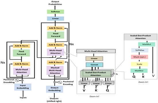
Figure 4.
Transformer architecture.
As shown in Figure 4, the transformer uses stacked self-attention and point-wise, entirely connected layers for both the encoder and decoder. Despite its many advantages, the transformer method has several drawbacks. When applied to high-dimensional sequences, transformers have a high computational cost [35]. Besides that, only fixed-length text strings can be dealt with by attention in the transformer method. Before being fed into the device as input, the text must be divided into a certain number of segments [36].
3.6. Proposed Model Architecture
In order to learn the relationship between future and past information efficiently in the Deep Learning method, it is necessary to process the forward and backward information simultaneously. Meanwhile, the traditional LSTM failed to learn from reverse order processing. Consequently, bidirectional LSTM (BiLSTM) has been introduced by putting two independent LSTMs together enabling them to have both backward and forward information about the sequence at every time step [37].
Unlike a traditional LSTM, the BiLSTM can run input sequence in two ways: forward layer from past to future and backward layer from future to past. By this approach, two hidden states from two LSTM models are combined with preserving information from both the past and future [38], which improve the long-term learning dependencies and the model’s accuracy.
In this work, a Single-Dense Layer BiLSTM was proposed and implemented to forecast PM2.5 concentration and to overcome the limitations of existing methods such as LSTM, CNN-LSTM, and Transformer based on time series data. The system consists of an input layer, a BiLSTM layer which contains LSTM backward layer, an LSTM forward layer, and a Single-Dense Layer BiLSTM. The architecture of our proposed model is depicted in Figure 5.
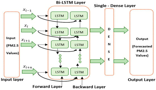
Figure 5.
A Single-Dense Layer BiLSTM architecture.
The input layer is regarded as the network’s starting point. The data samples of PM2.5 concentration are carried in the input layer as a time series. The BiLSTM layer contains two layers of LSTM are defined as the forward layer and backward layer. Forward layer acknowledges the input as ascending range, i.e., t = 1, 2, 3, …, T. Meanwhile, backward layer considers the input in descending order, i.e., t = T, …, 3, 2, 1. Therefore, and can be incorporated to produce output yt. The BiLSTM model is actualized with the following mathematical equations:
After the data is processed by the BiLSTM layer, it comes to a single-dense layer with a linear activation function to generate prediction with continuous values. The dense layer is an entirely connected layer, which means that all of the neurons in one layer are linked to those in the next layer [39]. Since a densely connected layer offers learning features from all combinations of the previous layer’s features, while a convolutional layer relies on consistent features with a limited repetitive area, a single-dense layer is used in this study.
3.7. Optimizer
In this experiment, adaptive moment estimation (ADAM) is used [40]. ADAM is a widely used approach for computing adaptive learning rates for each parameter of phase t. Thus, ADAM offers a practical learning algorithm. Moreover, this algorithm has gained much traction as one of the most reliable and efficient optimization algorithms for DL.
In ADAM, there are two crucial variables [41]. First, vt keeps an exponentially decaying average of past squared gradients. Second, mt keeps an exponentially decaying average of past gradients.
The first moment (the mean) and the second moment (the variance) of the gradients are estimated by vt and mt, respectively. When the gradients of two dimensions point are in the same direction, the mt increases, and when the gradients of two dimensions point in different directions, the mt decreases. ADAM changes the learning rates based on the parameters by adding vt, which performs more significant updates for small gradients and minor updates for large gradients. As a result, the moment estimates will be biased toward zero if these moving averages are initialized as vectors of zeros, particularly during the initial timesteps and when the decay rates are low [42]. The bias-corrected vt and mt are given as:
Here, and mean and to the power of t, respectively. ADAM’s choice of learning rate is one of its most significant features. The effective magnitude of the steps taken in parameter space at each timestep is roughly bounded by the step-size η, that is, |Δt| η [40]. The proper magnitude can be calculated ahead of time using this property.
4. Experiment and Results
4.1. Experiment with Hyperparameters Setting
To achieve the best output performance of the proposed model, the optimal values of hyperparameters are needed to be observed. The 64 nodes were selected to overcome several issues such as overfitting and underfitting; therefore, the correct number of nodes will affect the learning ability of the model: if it is too high, it may generate overfitting, while if it is too low, the complexity decreases, and the model may underfit [43]. A node in this proposed model is a computational unit containing the transfer function, weighted input connection, and output connection.
We used the ADAM optimizer because ADAM is a standard algorithm for training deep neural networks that uses a weighted average to monitor the relative prediction error of the loss function. Adam is based on the standard stochastic gradient descent (SGD) process, which does not account for outliers’ adverse effects [44]. One of the essential features of the ADAM optimizer is that it calculates both the momentum and the second moment of the gradient using exponential weighted moving averages (also known as leaky averaging) [45].
ADAM is a stochastic optimization technique that only needs first-order gradients and requires little memory. Individual adaptive learning rates for various parameters are calculated using estimates of the first and second moments of the gradients [46]. In the end, the hyperparameter that we emphasized in this paper is the dense layer which consists of one layer. We chose one single-dense to get optimal computational time in this proposed model. The list of values of optimal hyperparameters among all methods is provided in Table 1.

Table 1.
List of hyperparameters values of LSTM, CNN-LSTM, Transformer, and Single-Dense Layer BiLSTM.
Table 1 shows us a list of the hyperparameters used in this experiment. Because these four models have specific characteristics in their structure, some hyperparameter values cover all models, and there are some hyperparameter values that only one model has. For example, ReLU activation that only CNN-LSTM has, and nhead = 10 that only the Transformer model has. In this experiment, we chose a learning rate of 0.0001 for CNN-LSTM, since this value can give optimum results for this model.
4.2. Performance Criteria
We forecasted PM2.5 concentrations for the single day dataset, and the experiments used four parameters to assess the efficacy of our model: mean absolute error (MAE), mean square error (MSE), root mean square error (RMSE), and mean absolute percentage error (MAPE). Equations (25)–(28) give their meanings:
The average difference of the errors in a series of predictions is measured by MAE [47]. The absolute discrepancy between prediction and actual observation is averaged over the test sample using MAE, with all individual deviations given equal weight.
The difference between the fitted values and the actual data observation is measured with this MSE formula.
The formula of RMSE is the square root of the MSE. The RMSE can reveal whether a deviation has an impact on the model’s performance. Furthermore, the MAE and RMSE can be used to evaluate the model’s overall performance of forecasting [48], and higher forecasting accuracy can be associated with lower MAE and RMSE [49]. On the other hand, MAPE divides each error value by the actual value, resulting in a tilt: if the actual value at a given time point is low but the error is high, the MAPE value would be significantly influenced.
where denotes the real value, and denotes the predicted value, and n denotes the sample size. The smaller value of the MAPE will give better results for the forecasting [50].
4.3. Results and Comparison
In our experiment, the proposed Single-Dense Layer BiLSTM model was implemented to forecast PM2.5 concentrations with the same time series for three cases of time length, which are 5 min ahead, 30 min ahead, and 1 h ahead from 1-day, or 86,400 historical data points. We ran experiments for different outputs of the data, i.e., 5 min, 30 min, and hourly, to test the sequence learning models for short and long-term prediction.
Overall, the proposed Single-Dense Layer BiLSTM retains a low MAE, MSE, RMSE, and MAPE level at various sampling rates, which means that the forecasting accuracy can be assured even if the original sequence is resampled or a more extended period is used during data gathering.
The output of forecasting PM2.5 concentration for one hour ahead of using the proposed approach’s forecasting (a single-dense layer BiLSTM) algorithm is shown in Figure 6a–c. Figure 6a–c shows that the best result between train and validation loss occurs in the time of the 40th epoch. Moreover, the test and prediction results of the proposed system for one hour ahead are shown in Figure 7a–c. Figure 7a–c shows that the blue color line represents the actual values, and the orange color line represents the forecasting of the PM2.5 concentration. We can see from Figure 7c that the blue line and the orange line met at one point at the 40th epoch, which generates the values of MSE, RMSE, MAE, and MAPE at 8.18, 2.86, 2.47, and 0.014, respectively. These results attain the highest accuracy of the predicted value compared to three other methods.
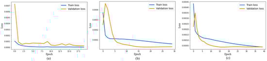
Figure 6.
Figure of loss function in 1 h ahead prediction for (a) 20 epochs, (b) 30 epochs, (c) 40 epochs.
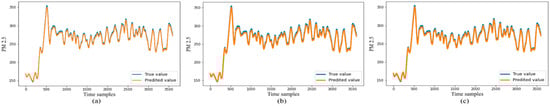
Figure 7.
Comparison of true value and predicted value in 1 h ahead prediction for (a) 20 epochs, (b) 30 epochs, (c) 40 epochs.
The fitting patterns of four different models to forecast PM2.5 concentration for five minutes ahead are depicted in Figure 8a–c. All the trend figures were taken to fit the same number of epochs (20, 30, and 40). Each model’s projected value moved closer to the actual value during its training phase. The proposed approach’s forecasting is the most accurate in terms of actual outcomes, as we can see from the closeness of the blue line, which represents the actual data, and the orange line, which means the forecasting data. We can see these results in more detail by referring to Table 2.
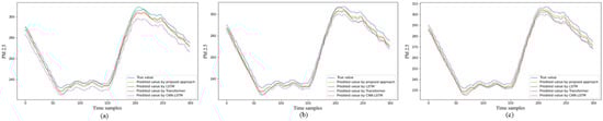
Figure 8.
Fitting trends of model for 5 min ahead prediction for (a) 20 epochs, (b) 30 epochs, (c) 40 epochs.
Table 2.
The 5 min ahead forecasting performance of LSTM, CNN-LSTM, Transformer models, and our proposed approach (Single-Dense Layer BiLSTM).
Table 2 shows that the MSE, RMSE, and MAE values in the LSTM, CNN-LSTM, and Transformer methods increased as the number of epochs executed on them increased. These results indicate that these three methods had overfitting. On the other hand, our proposed approach experienced a decrease in MSE, RMSE, and MAE values when the epoch was increased. These results indicate that our proposed method best fits the forecasting PM2.5 concentration 5 min ahead, considered to three other models.
Figure 9a–c shows the fitting trends, representing 30 min ahead forecasting from four different models. We ran 20, 30, and 40 epochs to all models; then, our proposed approach, represented in orange color line as the predicted value, achieved the closest distance with the blue color line, representing the true value. Table 3 illustrates further detailed results about what is shown from Figure 9a–c. In the LSTM model, the MSE and RMSE values increase when the number of epochs increases, while the MAE value decreases slightly at the 30th epoch and increases again at the 40th epoch. For the CNN-LSTM model, the values of MSE and RMSE was inclined in the 30th epoch, then declined in the 40th epoch, while its MAE gradually increased when the epoch increased. In the Transformer method, the values of MSE, RMSE, and MAE dropped in the 30th epoch and then hiked again in the 40th epoch. Meanwhile, even if our proposed approach had overfitting because the values of MSE, RMSE, and MAE increased along with the surging number of the epoch, it still achieved the best value compared with the three other methods.
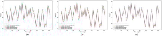
Figure 9.
Fitting trends of model for 30 min ahead prediction. (a) 20 epochs. (b) 30 epochs. (c) 40 epochs.
Table 3.
The 30 min ahead forecasting performance of LSTM, CNN-LSTM, Transformer models, and our proposed approach (Single-Dense Layer BiLSTM).
In order to study the forecasting accuracy at different time lengths and different epochs, we can refer to Table 2, Table 3 and Table 4, respectively.
Table 4.
The 1 h ahead forecasting performance of LSTM, CNN-LSTM, Transformer models, and our proposed approach (Single-Dense Layer BiLSTM).
Figure 10a–c depicts the fitting trends for one-hour forecasting from four different methods, each having 20, 30, and 40 epochs. Furthermore, in this time forecasting-length, our proposed approach, shown by an orange color line as the predicted value, came closest to the true value represented by a blue color line.
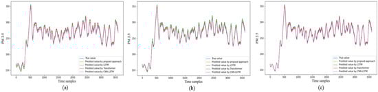
Figure 10.
Fitting trends of model for 1 h ahead prediction for (a) 20 epochs, (b) 30 epochs, (c) 40 epochs.
Table 4 further describes the results of what is illustrated in Figure 10a–c. In the LSTM and CNN-LSTM models, the values of MSE, RMSE, and MAE increased when the number of epochs surged from 20, 30, then 40, respectively. Meanwhile, the Transformer model and our proposed approach, Single-Dense Layer BiLSTM, presented values of MSE, RMSE, and MAE that declined when the epochs increased. Our proposed approach gains the lowest values of MSE, RMSE, and MAE.
Besides MAE, MSE, RMSE, and MAPE, Table 2, Table 3 and Table 4 also show us the training time results from the four different models. The LSTM model gained the fastest training time from epoch 20, 30, and 40 since it has the simplest structure compared to other methods, while the Transformer model had the longest training time because it has the most complex structure among all models in this study.
5. Conclusions
Since PM2.5 concentration can affect semiconductor factory air quality, there is a necessity for a framework to not only able to track air quality but also analyze data and provide visualization services. It is important to develop a reliable forecast system to ensure that people who work in the semiconductor factories know the potential air quality in cleanrooms. We integrated IIoT technology with the Single-Dense Layer BiLSTM method to build a PM2.5 forecasting system in this study. Furthermore, the Single-Dense Layer BiLSTM method was demonstrated for forecasting PM2.5 concentration to obtain MAE, MSE, RMSE, and MAPE, which were the lowest compared with LSTM, CNN-LSTM, and Transformer models for forecasting length 5 min ahead, 30 min ahead, and 1 h ahead. The proposed system can be applied to improve the optimum condition of PM2.5 concentration in the factory.
Even though we achieved positive results, some other works must be added in the future. This future research needs to add other size particulate matters such as PM0.5, PM1, PM5, and PM10. The final task entails developing a prescriptive analysis based on particulate matter forecasting services in a cleanroom semiconductor factory using the Single-Dense Layer BiLSTM.
Author Contributions
Conceptualization, A.T.P. and M.M.A.; methodology, A.T.P. and M.M.A.; data curation, A.T.P.; writing—original draft preparation, A.T.P. and M.M.A.; writing—review and editing, A.T.P. and M.M.A.; software, H.N., M.F.A. and M.H.R.; visualization, A.T.P., H.N., M.H.R. and M.M.A.; supervision, Y.M.J. All authors have read and agreed to the published version of the manuscript.
Funding
This work was supported by the Ministry of Trade, Industry and Energy (MOTIE) and Korea Institute for Advancement of Technology (KIAT) through the International Cooperative R&D program (Project ID: P0011880) and in part by MSIT (Ministry of Science and ICT), South Korea, under the ITRC (Information Technology Research Center) support program (IITP-2021-0-01396) supervised by the IITP (Institute for Information & Communications Technology Planning & Evaluation).
Data Availability Statement
The data presented in this study are available on request from the corresponding author. The data are not publicly available due to further research are on processing.
Conflicts of Interest
The authors declare no conflict of interest.
Abbreviations
| ADAM | Adaptive Momentum Estimation |
| ANN | Artificial Neural Network |
| BiLSTM | Bidirectional Long Short-Term Memory |
| CNN-LSTM | Convolutional Neural Network—Long Short-Term Memory |
| CPS | Cyber-Physical System |
| DL | Deep Learning |
| IIoT | Industrial Internet of Things |
| IoE | Internet of Everything |
| KDD | Knowledge Discovery in Database |
| LOCF | Last Observation Carried Forward |
| LSTM | Long Short-Term Memory |
| MAE | Mean Absolute Error |
| MAPE | Mean Absolute Percentage Error |
| ML | Machine Learning |
| MSE | Mean Square Error |
| NLP | Natural Language Processing |
| NOCB | Next Observation Carried Backward |
| PLC | Programmable Logic Controller |
| PM | Particulate Matter |
| PM0.5 | Particulate Matter of 0.5 µm |
| PM1.0 | Particulate Matter of 1.0 µm |
| PM2.5 | Particulate Matter of 2.5 µm |
| PM5 | Particulate Matter of 5 µm |
| PM10 | Particulate Matter of 10 µm |
| RDBMS | Relational Database Management System |
| RMSE | Root Mean Square Error |
| RNN | Recurrent Neural Network |
| SGD | Stochastic Gradient Descent |
References
- Yao, X.; Zhou, J.; Lin, Y.; Li, Y.; Yu, H.; Liu, Y. Smart Manufacturing Based on Cyber-Physical Systems and Beyond. J. Intell. Manuf. 2019, 30, 2805–2817. [Google Scholar] [CrossRef] [Green Version]
- Dafflon, B.; Moalla, N.; Ouzrout, Y. The Challenges, Approaches, and Used Techniques of CPS for Manufacturing in Industry 4.0: A Literature Review. Int. J. Adv. Manuf. Technol. 2021, 113, 2395–2412. [Google Scholar] [CrossRef]
- Agency, E.P. Particulate Matter (PM) Pollution. Available online: https://www.epa.gov/air-trends/particulate-matter-pm25-trends (accessed on 22 April 2021).
- Kim, C.; Chen, S.; Zhou, J.; Cao, J.; Pui, D.Y.H. Measurements of Outgassing From PM 2.5 Collected Collected in Xi’an, China Through Soft X-Ray-Radiolysis. IEEE Trans. Semicond. Manuf. 2019, 32, 259–266. [Google Scholar] [CrossRef]
- Semiconductor & Microelectronics. Available online: https://www.gore.com/products/industries/semiconductor-microelectronics (accessed on 22 April 2021).
- National Research Council. Industrial Environmental Performance Metrics: Challenges and Opportunities; The National Academies Press: Washington, DC, USA, 1999; ISBN 978-0-30906-242-8. [Google Scholar]
- Athira, V.; Geetha, P.; Vinayakumar, R.; Soman, K.P. DeepAirNet: Applying Recurrent Networks for Air Quality Prediction. Procedia Comput. Sci. 2018, 132, 1394–1403. [Google Scholar] [CrossRef]
- Chen, Y.C.; Lei, T.C.; Yao, S.; Wang, H.P. PM2.5 Prediction Model Based on Combinational Hammerstein Recurrent Neural Networks. Mathematics 2020, 8, 2178. [Google Scholar] [CrossRef]
- Xayasouk, T.; Lee, H.M.; Lee, G. Air Pollution Prediction Using Long Short-Term Memory (LSTM) and Deep Autoencoder (DAE) Models. Sustainability 2020, 12, 2570. [Google Scholar] [CrossRef] [Green Version]
- Li, T.; Hua, M.; Wu, X.U. A Hybrid CNN-LSTM Model for Forecasting Particulate Matter (PM2.5). IEEE Access 2020, 8, 26933–26940. [Google Scholar] [CrossRef]
- Wu, N.; Green, B.; Ben, X.; O’Banion, S. Deep Transformer Models for Time Series Forecasting: The Influenza Prevalence Case. arXiv 2020, arXiv:2001.08317. [Google Scholar]
- González, I.; Calderón, A.J.; Barragán, A.J.; Andújar, J.M. Integration of Sensors, Controllers and Instruments Using a Novel OPC Architecture. Sensors 2017, 17, 1512. [Google Scholar] [CrossRef] [Green Version]
- Xiong, J.; Bu, X.; Huang, Y.; Shi, J.; He, W. Safety Verification of IEC 61131-3 Structured Text Programs. IEEE Trans. Ind. Inform. 2021, 17, 2632–2640. [Google Scholar] [CrossRef]
- Molina-Coronado, B.; Mori, U.; Mendiburu, A.; Miguel-Alonso, J. Survey of Network Intrusion Detection Methods from the Perspective of the Knowledge Discovery in Databases Process. IEEE Trans. Netw. Serv. Manag. 2020, 17, 2451–2479. [Google Scholar] [CrossRef]
- Cao, K.; Liu, Y.; Meng, G.; Sun, Q. An Overview on Edge Computing Research. IEEE Access 2020, 8, 85714–85728. [Google Scholar] [CrossRef]
- Shivali, J.B.G. Knowledge Discovery in Data-Mining. Int. J. Eng. Res. Technol. 2015, 3, 1–5. [Google Scholar]
- Eyada, M.M.; Saber, W.; El Genidy, M.M.; Amer, F. Performance Evaluation of IoT Data Management Using MongoDB Versus MySQL Databases in Different Cloud Environments. IEEE Access 2020, 8, 110656–110668. [Google Scholar] [CrossRef]
- Prihatno, A.T. Artificial Intelligence Platform Based for Smart Factory. In Proceedings of the Korea Artificial Intelligence Conference, Pyeongchang, Korea, 16–18 December 2020. [Google Scholar] [CrossRef]
- Mendez, K.M.; Pritchard, L.; Reinke, S.N.; Broadhurst, D.I. Toward Collaborative Open Data Science in Metabolomics Using Jupyter Notebooks and Cloud Computing. Metabolomics 2019, 15, 1–16. [Google Scholar] [CrossRef] [Green Version]
- Morais, B.P. De Conversational AI: Automated Visualization of Complex Analytic Answers from Bots; Faculdade de Engenharia da Universidade do Porto: Porto, Portugal, 2018. [Google Scholar]
- Nguyen, V.-S.; Im, N.; Lee, S. The Interpolation Method for the Missing AIS Data of Ship. J. Navig. Port Res. 2015, 39, 377–384. [Google Scholar] [CrossRef] [Green Version]
- Hassani, H.; Kalantari, M.; Ghodsi, Z. Evaluating the Performance of Multiple Imputation Methods for Handling Missing Values in Time Series Data: A Study Focused on East Africa, Soil-Carbonate-Stable Isotope Data. Stats 2019, 2, 457–467. [Google Scholar] [CrossRef] [Green Version]
- Zhen, H.; Niu, D.; Wang, K.; Shi, Y.; Ji, Z.; Xu, X. Photovoltaic Power Forecasting Based on GA Improved Bi-LSTM in Microgrid without Meteorological Information. Energy 2021, 231, 120908. [Google Scholar] [CrossRef]
- Donald, F. Specht A General Regression Neural Network. IEEE Trans. Neural Netw. 1991, 2, 568–576. [Google Scholar]
- Meng, Y.; Jin, Y.; Yin, J. Modeling Activity-Dependent Plasticity in BCM Spiking Neural Networks with Application to Human Behavior Recognition. IEEE Trans. Neural Netw. 2011, 22, 1952–1966. [Google Scholar] [CrossRef]
- Singh, A. Anomaly Detection for Temporal Data Using Long Short-Term Memory (LSTM); Independent Thesis Advanced Level; School of Information and Communication Technology (ICT), KTH: Stockholm, Sweden, 2017. [Google Scholar]
- Zhao, B.; Li, X.; Lu, X. CAM-RNN: Co-Attention Model Based RNN for Video Captioning. IEEE Trans. Image Process. 2019, 28, 5552–5565. [Google Scholar] [CrossRef]
- Bengio, Y.; Simard, P.; Frasconi, P. Learning Long-Term Dependencies with Gradient Descent Is Difficult. IEEE Trans. Neural Netw. 1994, 5, 157–166. [Google Scholar] [CrossRef]
- Hochreiter, S.; Schmidhuber, J. Long Short-Term Memory. Neural Comput. 1997, 9, 1735–1780. [Google Scholar] [CrossRef] [PubMed]
- Ergen, T.; Kozat, S.S. Online Training of LSTM Networks in Distributed Systems for Variable Length Data Sequences. IEEE Trans. Neural Netw. Learn. Syst. 2018, 29, 5159–5165. [Google Scholar] [CrossRef] [PubMed] [Green Version]
- Zheng, C.; Wang, S.; Liu, Y.; Liu, C.; Xie, W.; Fang, C.; Liu, S. A Novel Equivalent Model of Active Distribution Networks Based on LSTM. IEEE Trans. Neural Netw. Learn. Syst. 2019, 30, 2611–2624. [Google Scholar] [CrossRef] [PubMed]
- Qin, D.; Yu, J.; Zou, G.; Yong, R.; Zhao, Q.; Zhang, B. A Novel Combined Prediction Scheme Based on CNN and LSTM for Urban PM2.5 Concentration. IEEE Access 2019, 7, 20050–20059. [Google Scholar] [CrossRef]
- Acquarelli, J.; Marchiori, E.; Buydens, L.M.C.; Tran, T.; van Laarhoven, T. Spectral-Spatial Classification of Hyperspectral Images: Three Tricks and a New Learning Setting. Remote Sens. 2018, 10, 1156. [Google Scholar] [CrossRef] [Green Version]
- Vaswani, A.; Shazeer, N.; Parmar, N.; Uszkoreit, J.; Jones, L.; Gomez, A.N.; Kaiser, Ł.; Polosukhin, I. Attention Is All You Need. Adv. Neural Inf. Process. Syst. 2017, 2017, 5999–6009. [Google Scholar]
- Khan, S.; Naseer, M.; Hayat, M.; Zamir, S.W.; Khan, F.S.; Shah, M. Transformers in Vision: A Survey. arXiv 2021, arXiv:2101.01169. [Google Scholar]
- Yates, A.; Nogueira, R.; Lin, J. Pretrained Transformers for Text Ranking: BERT and Beyond. In Proceedings of the WSDM 2021—14th ACM International Conference on Web Search and Data Mining 2021, Jerusalem, Israel, 8–12 March 2021; pp. 1154–1156. [Google Scholar] [CrossRef]
- Xie, J.; Chen, B.; Gu, X.; Liang, F.; Xu, X. Self-Attention-Based BiLSTM Model for Short Text Fine-Grained Sentiment Classification. IEEE Access 2019, 7, 180558–180570. [Google Scholar] [CrossRef]
- Ronran, C.; Lee, S.; Jang, H.J. Delayed Combination of Feature Embedding in Bidirectional Lstm Crf for Ner. Appl. Sci. 2020, 10, 7557. [Google Scholar] [CrossRef]
- Rampurawala, M. Classification with TensorFlow and Dense Neural Networks. Available online: https://heartbeat.fritz.ai/classification-with-tensorflow-and-dense-neural-networks-8299327a818a (accessed on 1 June 2021).
- Kingma, D.P.; Ba, J.L. Adam: A Method for Stochastic Optimization. In Proceedings of the 3rd International Conference on Learning Representations, ICLR 2015—Conference Track Proceedings, San Diego, CA, USA, 7–9 May 2015; pp. 1–15. [Google Scholar]
- Yu, X. Deep Learning Architecture for PM2.5 and Visibility Predictions; Delft University of Technology: Delft, The Netherlands, 2018. [Google Scholar]
- Ruder, S. An Overview of Gradient Descent Optimization Algorithms. arXiv 2016, arXiv:1609.04747. [Google Scholar]
- Hameed, Z.; Garcia-Zapirain, B. Sentiment Classification Using a Single-Layered BiLSTM Model. IEEE Access 2020, 8, 73992–74001. [Google Scholar] [CrossRef]
- Yang, H.; Pan, Z.; Tao, Q. Robust and Adaptive Online Time Series Prediction with Long Short-Term Memory. Comput. Intell. Neurosci. 2017, 2017, 9478952. [Google Scholar] [CrossRef] [PubMed] [Green Version]
- Zhang, A.; Liption, Z.C.; Li, M.; Smola, A.J. Dive into Deep Learning. Available online: https://d2l.ai/chapter_optimization/adam.html (accessed on 30 April 2021).
- Guo, C.; Liu, G.; Chen, C.H. Air Pollution Concentration Forecast Method Based on the Deep Ensemble Neural Network. Wirel. Commun. Mob. Comput. 2020, 2020, 8854649. [Google Scholar] [CrossRef]
- Jonathan, B.; Rahim, Z.; Barzani, A.; Oktavega, W. Evaluation of Mean Absolute Error in Collaborative Filtering for Sparsity Users and Items on Female Daily Network. In Proceedings of the 1st International Conference on Informatics, Multimedia, Cyber and Information System, ICIMCIS 2019, Jakarta, Indonesia, 24–25 October 2019; pp. 41–44. [Google Scholar] [CrossRef]
- Zhang, Y.F.; Thorburn, P.J.; Xiang, W.; Fitch, P. SSIM—A Deep Learning Approach for Recovering Missing Time Series Sensor Data. IEEE Internet Things J. 2019, 6, 6618–6628. [Google Scholar] [CrossRef]
- Ait-Amir, B.; Pougnet, P.; El Hami, A. Meta-model development. In Embedded Mechatronic Systems 2; El Hami, A., Pougnet, P.B.T., Eds.; ISTE: London, UK, 2020; pp. 157–187. ISBN 978-1-78548-190-1. [Google Scholar]
- Swamidass, P.M. MAPE (Mean Absolute Percentage Error) MEAN ABSOLUTE PERCENTAGE ERROR (MAPE) BT—Encyclopedia of Production and Manufacturing Management; Swamidass, P.M., Ed.; Springer: Boston, MA, USA, 2000; p. 462. ISBN 978-1-4020-0612-8. [Google Scholar]
Publisher’s Note: MDPI stays neutral with regard to jurisdictional claims in published maps and institutional affiliations. |
© 2021 by the authors. Licensee MDPI, Basel, Switzerland. This article is an open access article distributed under the terms and conditions of the Creative Commons Attribution (CC BY) license (https://creativecommons.org/licenses/by/4.0/).