Article

A Predictive Control Strategy for Energy Management in Micro-Grid Systems

by
Abdellatif Elmouatamid
1,2,*,
Radouane Ouladsine
1,
Mohamed Bakhouya
1,
Najib El kamoun
2 and
Khalid Zine-Dine
3
1
LERMA Lab, College of Engineering and Architecture, International University of Rabat, El Jadida 11100, Morocco
2
STIC Laboratory, Faculty of Sciences, Chouaïb Doukkali University, El Jadida 24000, Morocco
3
Faculty of Science, Mohammed V University, Rabat 10000, Morocco
*
Author to whom correspondence should be addressed.
Electronics 2021, 10(14), 1666; https://doi.org/10.3390/electronics10141666
Submission received: 20 April 2021 / Revised: 14 May 2021 / Accepted: 20 May 2021 / Published: 13 July 2021
(This article belongs to the Special Issue Smart Embedded Systems and Applications)

Abstract

:
The integration of renewable energy sources (RES) was amplified, during the past decades, in order to tackle the challenges related to energy demands and CO2 increases. Recently, many initiatives have been taken by promoting the deployment and the usage of micro-grids (MG) in buildings, as decentralized systems, for energy production. However, the variable nature of RESs and the limited size of energy storage systems require the deployment of adaptive control strategies for efficient energy balance. In this paper, a generalized predictive control (GPC) strategy is introduced for energy management (EM) in MG systems. Its main objective is to efficiently connect the electricity generators and consumers in order to predict the most suitable actions for energy flow management. In fact, based on energy production and consumption profiles as well as the availability of energy storage systems, the proposed EM will be able to select the best suitable energy source for supplying the building’s loads. It will efficiently manage the usage of energy storage and the utility grid while maximizing RESs power generation. Simulations have been conducted, using real-sitting scenarios, and results are presented to validate the proposed predictive control approach by showing its effectiveness for MG systems control.

1. Introduction

In the past decades, energy management (EM) systems have been proposed for improving the global performance of buildings while maintaining a suitable occupants’ comfort. Recent studies showed that energy consumption in buildings could be efficiently reduced by deploying micro-grid (MG) systems [1]. The aim is to minimize the electrical bill’s cost while extending the lifetime of the system’s components (e.g., converters, batteries, and fuel cells). Generally, an EM system incorporates control approaches and functions, which maximize the MG system’s efficiency and minimize energy consumption. In some cases, control approaches use single-objective function procedures (e.g., maximizing the quality of services). Without considering different operating constraints, these procedures are easier to implement and to deploy in real-sitting scenarios. Moreover, an EM control strategy, which takes into consideration only the energy availability within MG components (e.g., energy sources, storage devices, utility grid), could be implemented by simple algorithms. These algorithms implement procedures that switch, at each time, from RES to storage devices or to the traditional electrical grid (TEG). For instance, actual commercial inverters are able to manage the interconnection between renewable energy sources (RESs), energy storage systems, and the utility grid by incorporating a single-objective function. In particular, the MG system’s EM takes into consideration only the availability of the electricity for being supplied to buildings loads. For instance, the inverter can use either batteries or the utility grid without taking into account other parameters, such as the actual electricity cost as well as batteries charge/discharge cycles. However, high battery charge/discharge cycles, in a limited time, could decrease their performance, which impact on the system’s profitability [2]. In other cases, controllers can interact, in real-time, with energy sources generators (e.g., solar, wind) in order to limit the power generation (limited power point tracking). The aim is to ensure the quality of electrical services (e.g., frequency, voltage), and consequently minimizing the profitability of MG system’s components. Despite their advantages, they could have, however, negative impacts on the batteries’ lifecycle and system’s profitability. Therefore, context-awareness principles and predictive analytics could be exploited for developing context-driven and predictive control approaches, such as generalized predictive control (GPC) [3]. It is worth noting that GPC approaches are not new and have been applied in grid and EM control applications. However, due to recent development of information and communication technologies (ICT), these approaches could be deployed in real-sitting scenarios by using machine learning algorithms and recent artificial intelligence techniques. The latter are mainly used to forecast/predict control input parameters, such as power production and consumption. Furthermore, the improvement of microcontrollers and microprocessors offers more advantages for the predictive control deployment in embedded devices, such as in power converters [3,4].
The work presented in this paper introduces a predictive control approach for EM in MG systems. In fact, due to the development of information and communication technologies (e.g., machine learning, IoT/big-data, smart metering) with its integration to the energy management component, the predictive control can have a new revolution using machine learning algorithms to forecast the input control parameters. In addition, the improvement of microcontrollers and microprocessors offers more advantages for the predictive control deployment. The proposed control approach is capable to manage energy flows in MG systems using data prediction and forecasting algorithms. Mainly, collected data (e.g., power production, power consumption, batteries’ state of charge) can be used to train machine-learning algorithms in order to generate the control input parameters. The main objective is to improve the performance of existing predictive control methods by using recent Internet of things (IoT) and big-data technologies [4,5,6]. In fact, unlike the above-mentioned approaches, the proposed control approach considers multiple objective functions, which take into consideration batteries charge/discharge cycles as well as the electricity price forecasting. Its main aim is to ensure, in an optimal way, the continuous electricity supply, from different installed sources (e.g., RESs, batteries, TEG), to building’s services. The proposed approach is based on the GPC model, which is able, based on forecasted inputs values, to generate a sequence of future control actions over a prediction horizon. This requires an advanced metering infrastructure, which allows measuring and predicting all inputs values. Therefore, an MG was deployed together with an IoT/big-data platform in order to conduct experiments and validate developed models. As depicted in Figure 1, the MG system contains RESs and battery storage systems, which are connected together with the utility grid in order to supply the electrical energy to building’s loads (e.g., lighting, ventilation). The IoT/big-data platform was developed and deployed in order to allow measuring and forecasting RESs power generation, loads consumption, and batteries state of charge (SoC) [7,8]. An embedded system was also developed and contains mainly a microcontroller, which is connected to several sensors (e.g., current, voltage) and actuators for performing selected and generated actions by the GPC-based controller. This later, based on forecasted values, allows switching between different energy sources, batteries, and the utility grid. The GPC is deployed for conducting experiments and compared against a model predictive control (MPC) strategy, as already developed in our previous work [3].
The remainder of this paper is organized as follows. Section 2 presents a brief state of the art of predictive control deployment for EM and power converter control. Materials and methods are presented in Section 3, by putting more emphasize on system modeling for the GPC algorithm deployment together with its optimization functions and constraints. The results and interpretations are discussed in Section 4, by deploying the investigated GPC model and control strategy. Conclusions and perspectives are outlined in Section 5.

2. Related Work

Appropriate EM systems, incorporating control strategies, are required for reliable and robust operation of MG systems. These control strategies must take into consideration the nature of installed RES, storage systems, and their interconnection to the electrical networks. Figure 2 presents the future architecture of MG systems together with the required control strategies, which could be adopted at each system’s level. It highlights the role of participating entities in this new smart electricity network (e.g., manufacturers, electricity operators, consumers). However, the most significant challenge of this new MG system’s architecture is the development and the deployment of suitable control strategies. These strategies are required for efficient energy balance while ensuring a high level of power quality and favoring the active integration of prosumers in its related emerging electricity market. In addition, within this new MG system architecture, control strategies must take into consideration the multiple disturbance variables and constraints, which are present at different time scales.
Recently, numerous approaches have been proposed and could be classified according to the MG system’s layers, as depicted in Figure 2, including primary, secondary and tertiary controls. At the primary control level, the power converter is connected to RESs and interacts directly with the EM system. This later is responsible for improving the frequency and the voltage stability by preventing circulating the current among converters. Generally, frequency- and voltage-power droop controls are deployed as the primary controller [9]. The droop control method is often used at this level in order to emulate physical behaviors that make the system stable and more damped [10]. In fact, the load changes in the MG cause direct current (DC) link voltage variation and the droop controller can change the output power of the converter by interacting on the voltage variation. It includes a virtual impedance control loop to emulate physical output impedance. Moreover, in this hierarchical layer, the control signals are sent in milliseconds [11] in order to stabilize the internal MG buses, to address some power quality issues, and to track the maximum power generated by RESs. Due to communication time, which should be minimal or negligible, the generated control signals are based only on local measurements (e.g., voltage, current).
At the secondary control layer, the controller ensures, after system load variation, that the power levels (e.g., frequency, voltage, current) into the MG systems are within the required standards values. The standardization is considered by the converters’ manufacturers in order to ensure a seamless MG connection or disconnection to or from the utility grid. It can include a synchronization control loop in order to avoid voltage and current violations by sending modified power references to the distributed energy sources. In addition, this control layer is considered as a mediator between the third and the primary layers. In fact, the second layer corrects the frequency and voltage deviations between the optimization upper reference signals and real MG’s measurements, which have not been solved by the primary control. In this context, this control level can be formulated as a redundant optimization problem in order to achieve more accurate outputs [12]. As shown in Figure 3, this control level is considered as a lower controller layer. It can be designed to reach the optimal power references toward the primary control layer, which is responsible for generating the commands (e.g., turn-on, switch-off) to each commendable unites in the converter to reach the desired set point. At this layer, the EM system takes its decisions based on dedicated inputs, mainly RES power generation, power consumption, battery SoC, weather forecast, and the energy price estimation [13,14]. Generally, the control strategy is designed as an optimization problem taking into account both discrete (e.g., RESs disconnection decisions, the operation state) and continuous variables (e.g., bus voltage, active and reactive power). This optimization is most often solved using integer linear programming techniques [15,16,17].
Unlike primary and secondary control layers, the tertiary control manages the power flow between the MG and the electrical grid on the one hand and between the MG and eventually neighboring MG on the other hand. This control, throughout the EM, allows the optimal operation and planning of the MG system taking into consideration the second layer control outputs [9]. The main objective functions of this control layer are to minimize the daily operating costs, to maximize the profitability of the installed RES system, and to improve the self-consumption of the RESs. These functions are formulated as optimization problems by including the energy cost function and environmental/operational system’s constraints, as shown in Figure 3. By considering those constraints, the optimization problem could be solved using convex optimization techniques (COT), which compute the appropriate MG system’s operations and daily cost. The commands and actions in this layer are updated every second, minute, hour, or even daily, depending on deployed control strategies. In addition, the power generation and consumption together with batteries’ SoC have to be measured and processed in order to generate new reference values to the controller. Recently, predictive approaches have been proposed for advanced systems’ control according to defined constraints. Their aim was to develop predictive controllers for efficient energy flow in MG systems. These controllers could forecast future actions and decisions, but they require forecasted inputs’ values (e.g., power consumption/production). With recent progress in IoT and big-data technologies together with machine learning and artificial intelligence techniques, it is now possible to deploy sensors for gathering contextual data [13]. These data could be processed and used for predicting n-step-ahead values. Therefore, the forecasted values are the main inputs that are used by predictive control approaches for generating the most suitable and future actions [5].
MPC and GPC are the well-known approaches having the capabilities of predicting future events and forecasting right control decisions accordingly. In fact, they have the ability to incorporate optimization mechanisms, which allows integrating system’s constraints and disturbances in forecasted control decisions. For instance, the GPC is widely used in advanced control applications, such as in EM and buildings’ automation systems [6,18,19,20]. For example, the work presented in [21] introduced a home EM system for battery storage and PV systems. The proposed planning, for the optimal operation strategy, is expressed as a stochastic mixed-integer nonlinear programming. The power generated by the PV system is considered as an uncertain parameter and modeled by a probability distribution function. The battery storage system is used to store energy during off-peak/low-cost hours and discharge energy during on-peak/high-cost hours. However, the main limitation of this EM strategy is the passive reaction of the system with the cost and the peak demand variability. It is programmed by a fixed time interval, which represents the predefined periods of on-peak and high-cost. In addition, it is not defined by an active function for the interactive variability of the cost and the electricity demand. Moreover, authors in [20] proposed an adaptive and dynamic optimization technique based on the stochastic MPC approach. The proposed EM approach is applied for distributed energy resources scheduling problem for a set of smart homes with different sources of energy. Its aim is to address the uncertainty and variability issues of the PV power generation. This study is designed for large-scale smart houses by taking into consideration their cooperation with their surrounding neighbors. Another interesting work is presented in [22], in which the authors proposed an EM system using the MPC where a simple state-space model is used for the performance modeling of a MG system. This work considered the RESs power production and the consumption as measured disturbances parameters for the EM system. Therefore, the storage systems and the cost are modeled as constraints for the MG system, which are solved by the state-space equations. In addition, other works are presented in literature, which refer to optimal control of RES in MG systems, considering hybrid storage systems, as detailed in [23]. In [24], the authors used the MPC for optimal control of distributed energy resources with a battery storage system. In other works, the MPC is used for EM of MG systems that are connected to the charging station for electrical vehicles [25,26,27]. Generic MPC models are introduced in [28,29] for economic optimization in MG systems. Another interesting work is presented in [30], where authors proposed a MPC methodology to manage the power quality of MG system. The power converters are regulated in order to achieve the requirement by applying the algorithm to a four-wire three-phase voltage source inverter, which works as master of a microgrid with unbalanced and non-linear loads and generators connected.
It is worth noting that the MPC family was proposed for electronic power, and especially for power converter control. The GPC is one of the continuous control set MPC (CCS-MPC) methods that calculate a continuous control command in order to generate the desired output of the power converter. The CCS-MPC models have a lower computational cost than other existing methods, such as the finite control set (FCS-MPC), optimal switching vector (OSV-MPC), and optimal switching sequence (OSS-MPC) [31]. It can be used for a long predictive horizon by calculating the control actions beforehand and then limiting the online computation burden. Mainly, the calculation time is the main factor for the deployment of MPC control families. In past decades, the development of computing units and the integration of ICTs and machine-learning algorithms for power electronic applications encourage the use of predictive control for power converters. For instance, in [32,33], a FCS-MPC is used for current control of three-phase inverter. It is studied in [34] for a multiphase inverter, in [35,36] for a multilevel inverter, and in [37,38] for a matrix converter. For more details, we refer readers to recent interesting reviews, which are related to predictive control applications in power electronics [39,40,41,42]. The work presented in [43] investigated decentralized MPC based hierarchical control scheme with both primary and secondary level for an islanded alternative current (AC) MG system. The aim was to address power quality and unequal power sharing problems. The control scheme consists of an inner control loop, primary and secondary control. The FCS-MPC is incorporated in the inner loop to track the reference voltage and fix the capacitor voltage in each distributed generator unit. Primary control comprises of virtual impedance loop and droop control to manage the power flow and power sharing among distributed generator systems. Moreover, state space predictor based secondary control is proposed for regulating frequency of the MG and node voltage to their nominal values in islanded operation. In [40], authors reviewed the system components, modeling, and control of MG for future smart buildings. An overview of MG control and optimization is given in terms of optimization methods, constraints, and objectives. Mainly, depending on the scale of the controlled system, several works are presented. In fact, for some research works, the control constraints and the objective functions are investigated for large scale MG systems. For example, authors in [44] presented a good control strategy based on an economic MPC approach for community-based MG systems. The control strategy is applied to design the central controller of a large number of MG systems. It mainly showed the capability to efficiently deal with multivariable dynamic constrained systems and to predict properly its actions in order to achieve the optimal performance according to user defined cost functions. Authors realized a comparative analysis of both heuristic and MPC approaches. Reported results showed that the MPC approach has a strong impact on the overall cost of the system. It is able to guarantee a 20-year lifetime of the battery avoiding then its replacement while satisfying the other required criteria.
In this work, a hierarchical approach is proposed to control the energy flow in single MG systems. Unlike the works that investigated the control approaches for multiple MG systems, this work focuses on the EM of a single MG system with the perspective to develop a smart inverter, which can execute predictive control approaches. More precisely, an EM system is deployed based on GPC model in order to manage the operation of such MG and in particular its interaction with the main utility grid. A power converter is then modeled and controlled by a GPC model for ensuring the interaction with the grid. An optimization function with dedicated constraints is modeled for both secondary and tertiary layers. For the second layer, the charge/discharge cycle of the battery and the maximum power extracted from RESs are designed as the main constraint to be optimized by the GPC model, while for the tertiary layer the electricity price is integrated as an input parameter for the controller.

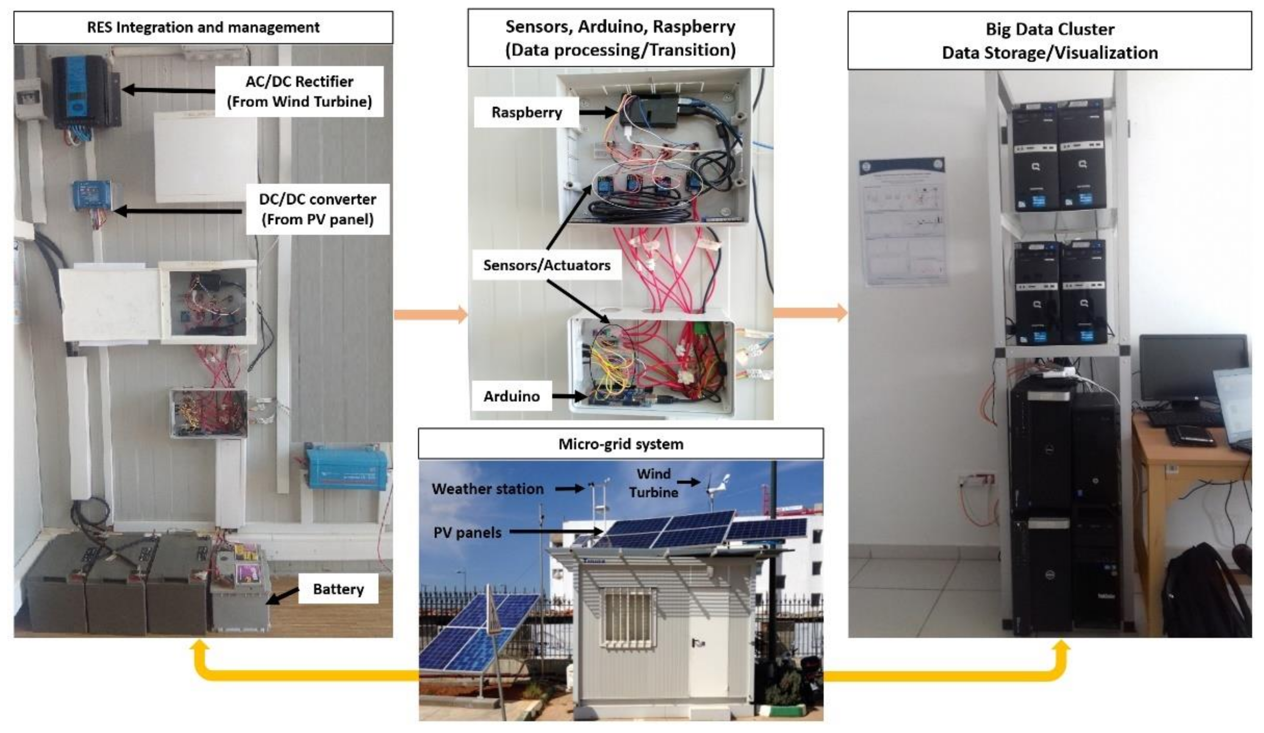
3. Materials and Methods

The MG system is connected together with the utility grid and storage systems in order to supply the power to the building’s load. Furthermore, the MG system could operate in either connected or standalone modes while ensuring frequency and voltage quality. This section provides more details of the MG system modeling for the GPC integration. The GPC model is presented by focusing on its key elements, which we have considered in the present study.

3.1. Control Strategy Design and GPC Integration

The GPC is a predictive approach that allows computing and predicting the suitable actions for being performed according to forecasted and contextual information/constraints of MG systems. It can be classified with advanced process control families with less variation in process variables. Its main concept, as depicted in Figure 4a, is described as follows. Based on a predefined model of the MG system, optimal future actions (controls/commands) are computed to reach the desired set point according to the defined constraints and optimization functions. These functions consider future errors, constraints, and control parameters (Figure 4b). An interesting work is presented in [45] about model predictive control for buildings. The work provides a unified framework for model predictive building control technology with a focus on the real-world applications.
As described in Figure 4a, the predictor generally calculates, for each instant t , the predictions of the dynamic evolution of the process y t + 1 ,   ,   y t + N T throughout the defined horizon, N s t e p s ahead. This prediction is based on the dynamic parameters, which are measured at t, as well as the future control system’s regulation u t ,   u t + 1 ,   ,   u t + N T , along the prediction horizon N . The future control actions are then generated in order to optimize the desired cost function by resolving, at each defined time step, the predefined constraints. The designed cost function keeps the system’s output at t + k as close as possible to the defined setpoint. This setpoint dictates the output evolution accordingly by considering the evolution of the constraints position (Figure 4b). As is explained in Figure 4b, the system should be controlled to reach the set point by calculating the minimum trajectory from the actual measurements respecting the cost function to be minimized and avoiding the obstacles (constraints) at the same time. Generally, the cost function takes the form of a quadratic function of the errors between the predicted output and the set point [46].
For GPC integration within the MG system, we focus only on secondary and tertiary control. The former control considers that the EM supervises the MG system by gathering the required data from its entities, mainly RES, batteries, and loads. It mainly manages the energy for both grid-connected and islanded modes with reliable and secure operation. Accordingly, the controllable units of the studied MG system, in both modes, are modeled by a state-space equation, described in Equation (1), where x t is the system state, u t is the vector of manipulated variables, y t is the output vector, and A ,   B ,   C are respectively the system matrix, the control matrix, and output matrix.
x t + 1 = A x t + B u t y t = C x t
In the secondary layer, we have incorporated the GPC within the EM in order to generate suitable control actions for efficient power Demand/Response balance. More precisely, the batteries SoC is controlled by the GPC strategy according to the variability of predicted power production, power consumption, and electricity cost. In fact, the power generated by the RESs and the power consumption are considered as disturbances sources for the MG system during its operation. Mainly, the storage system is the main unit used to smooth power fluctuations in MG systems and the main parameter considered for studies in the literature is the SoC variability [47]. For that, the control strategy is designed based on the SoC variability in a MG system, which is used to smooth the power generation on the one hand, and to minimize the electricity price for another hand. Therefore, batteries’ SoC could be modeled by a state-space equation while the variability of these controllable parameters is considered because of the disturbances variation, which is described as follows:
P b a t = P R E S P l o a d ;   i f   0 P R E S   a n d   S o C m i n < S o C S o C m a x P l o a d ;   i f   P R E S = 0   a n d   S o C m i n < S o C
where P b a t is the power generated or extracted from the battery, P R E S is the power generated by RES, P l o a d is the load demand, S o C m i n is the minimum batteries SoC (to avoid a deep discharge), and S o C m a x is the SoC when the batteries are fully-charged.
Generally, the controller cannot manipulate the disturbances of the system. Hence, in our GPC model, the RES power generation and the load consumption are represented as measured system’s disturbances. These disturbances can be computed using actual measured power production/consumption, which are in turn affected by external disturbances (e.g., weather conditions, occupant’s activities). The deployed IoT/big-data platform, as stated above, could handle this task by forecasting these disturbance parameters (i.e., RES, load power), and consequently, minimizing the GPC prediction errors [4,5]. In fact, if the disturbances can be measured or predicted, their influence on the system’s output can be included in the GPC model. This allows anticipating their effect on the control command. Like any predictive control model, the GPC can reject disturbances according to the feedback mechanism. In this way, the GPC can inherently include a feed-forward effect. Therefore, the d ( t ) disturbances’ effect is added to the state-space formulation (Equation (1)) and the equivalent dynamic model is then written in Equation (3), where B d is the matrix, which quantifies the effect of the disturbances on the system states, and d t = P R E S P l o a d combines the disturbances into one variable.
x t + 1 = A x t + B u t + B d d t y t = C x t
As stated above, the main aim of the GPC is to control the battery charging/discharging power. In fact, the GPC regulates the battery state in order to reach the operating goal (i.e., demand/response balance) and to make the right decision: charge, discharge, or battery-at-rest. At a first step, these decisions are made depending on the conditions, which are mentioned in Equation (2). It is worth noting that for modeling the SoC dynamics, the disturbances could be indirectly integrated in the control variables. More precisely, the future values S o C t + 1 can be calculated by accumulating the actual S o C t and the battery charge/discharge current, as described in Equation (4), where I b a t = I R E S I l o a d is the batteries’ charge/discharge current, I R E S and I l o a d are respectively the PV and load current, C is the nominal capacity of the battery, and Δ t is the operating period.
S o C t + 1 = S o C t + I b a t t . Δ t / C
By considering the S o C t as the system state, Equation (4) can be rewritten by Equation (5), where x t is the system state, A = 1 , and the I b a t t = B is the system input.
x k + 1 = A x k + B U k
By interpolation, Equation (4) to n-step-ahead, the above-mentioned form (Equation (5)) could be rewritten in a matrix form as follows:
x k + 1 x k + n = A A n   x k + B 0 0 A B B 0 A n 1 B A B B U k U k + n + 1
Mainly, for the input vectors, we consider the following change:
U   k = U k 1 + Δ U k U   k + 1 = U k + Δ U k + 1 = U k 1 + Δ U k + Δ U k + 1 U k + n 1 = U k 1 + Δ U k + Δ U k 1 + + Δ U k + n 1
The input vectors u k could be similarly rewritten as follows:
U k U k + 1 U k + n = 1 1 n   U k 1 + 1 0 0 1 0 1 1 1 Δ U k Δ U k + 1 Δ U k + n + 1
It is equivalent to:
U ¯ = I 1 U k 1 + I 2 Δ U ¯ k
We can then obtain the following predictive model by replacing Equation (9) in Equation (6):
X ¯ = A ¯ x k + B ¯ I 1 U k 1 + B ¯ I 2 Δ U ¯ k Y ¯ = C ¯ x k + D ¯ I 1 U k 1 + D ¯ I 2 Δ U ¯ k
The main constraint, we have considered in the secondary control layer, is related to the batteries’ charge/discharge (i.e., the SoC stays at its maximum as much as possible). Therefore, the aim is to minimize the given objective function E N (Equation (12)) within a prediction horizon N . It should be noted that the prediction horizon N has a length strictly superior to the control horizon n . However, for some scenarios, when a machine-learning algorithm is used to generate the control input parameters, the prediction horizon can be minimized and the optimization function can generate its optimal behavior based on the forecasted values [3]. However, in order to get the control sequence Δ U , the criterion that will be optimized is described by Equation (13). It is composed of the quadratic error and the command level.
Y r e f = S o C m a x k + 1 ,   S o C m a x k + 2 , , S o C m a x k + N
E N = S o C m a x 1 1 N S o C t SoC t SoC t + N
J = 1 2 E Q E T + Δ U ¯   R   Δ U ¯ T
Alike the secondary control, which manages the energy for both grid-connected and islanded modes with reliable and secure operation, the tertiary control tackles all issues related to the interconnection between the MG system and the utility grid. It mainly adjusts the power set point in order to efficiently manage the power flows by having the possibility to interconnect multiple MG systems. This control layer is mainly considered at the same time as a part of the main grid and the MG system. Under this control, several constraints could be included as a cost function for the efficient management of MG systems. Examples are the electricity price (i.e., the cost for purchasing electricity from the utility grid), the system’s profitability (i.e., daily operation costs of the battery storage system and RESs), and the revenue related to the excess energy, which is injected to the utility grid (i.e., selling energy to the neighboring MG systems).
In this work, the electricity price is considered as a fundamental constraint, which is shared between the secondary and the tertiary control layers. In fact, by interpolating this constraint in both layers, the control actions must be generated according to the electricity price variability. The cost function variability used in our work follows the energy price, as presented by the European foundation [48]. In fact, the following control strategy is adopted. When the electricity price is inexpensive, the control strategy could charge the batteries from the main grid for being used during the morning peak consumption, otherwise, the batteries and RESs could be used to supply the power to building’s loads while the surplus can be injected into the utility grid. Mainly, when the price is less than a defined threshold value, a simple conditional control strategy could be deployed to balance the power flow by providing the priority to RESs and the utility grid than batteries, otherwise, the batteries and the RESs have the priority to supply the building’s loads, as shown in Figure 5. In all cases, the battery can be charged from either RESs or the utility grid according to the daily electricity price variation. In order to include the above-mentioned constraints into the GPC, we use an incremental model by considering Δ u t = u t u t 1 as the control decision variable, and, therefore, the state-space equation could be represented as in Equation (14), where the new state vector is z t = x t . u t 1 T and the matrices M ,   N ,   a n d   Q are obtained by comparing Equation (3) and Equation (14).
z t + 1 = M z t + N   Δ u t + N d d t y t = Q z t
It is worth noting that the basic theory of GPC is to compute a sequence of future control actions in order to minimize a multi-stage cost function, which is defined over a prediction horizon. The criterion to be optimized is the expectation of quadratic function that measures the distance between the system’s outputs prediction and the reference sequence over a prediction horizon. In the presented state-space equation (Equation (14)), the prediction includes the estimated disturbances (i.e., RESs production, load consumption). The GPC original algorithm is extended to include the cases of measurable disturbances and to change in the predictor. In fact, by considering a system that operates around a practical set point, the single-input single-output of the system plant can be described by Equation (15), after linearization, as follows:
A z 1 y t = z d B z 1 u t 1 + C z 1 . e t Δ
This model is known as a CARIMA (controller auto-regressive integrated moving-average), where Δ = 1 z 1 , e t is a zero mean white noise, d is the dead time of the system, and the polynomials A ,   B ,   a n d   C , in the backward shift operator z 1 , are presented by:
A z 1 = 1 + a 1 z 1 + a 2 z 2 + + a n a z n a B z 1 = b 0 + b 1 z 1 + b 2 z 2 + + b n b z n b C z 1 = 1 + c 1 z 1 + c 2 z 2 + + c n c z n c
The most transfer function model, used by the GPC method, is the commonly used model, called CARIMA model. This form of plant model is formulated in a way that the uncertainty is added into a good representation, so that slow variation of disturbances could have non-zero steady-state. We then synthetize from the CARIMA model a one-step-ahead prediction equation that represents a set of simultaneous prediction equations. The unified GPC algorithm based on CARIMA model can be implemented using model parameters without the need of solving Diophantine equations. The procedure of unified GPC starts by estimating the model parameters and choosing the appropriate values of the maximum and the minimum costing horizon. The model calculates the j -th step response parameter and predicts the plant output assuming future controls equal u t 1 [49]. Therefore, the main objective of predictive control is to predict the future control actions u t , u t + 1 , and u t + i in such a way that the future system’s output is driven to reach the set point. At the end, the unified GPC calculates the future control increment, extract the first element Δ u t , and computes the u t . This step is inspired from the model presented in [49]. Basically, the GPC model consists of applying a sequence of control actions in order to minimize a defined multi-objective cost function. It is worth noting that this vector is generated by a machine-learning algorithm, which is mainly used to forecast the RESs power generation and load consumption [13,50,51]. Consequently, the GPC predictor can reject the effect of these disturbances, along the horizon N , by providing a feed-forward effect. Within this context, the prediction is generated by considering only the cost function, which is modeled by the electricity price as well as the cost associated to the energy mainly used to keep the batteries’ SoC at its maximum. Therefore, the constraint defined for the tertiary level control can be written as follows:
J N 1 , N 2 ,   N u = j = N 1 N 2 | u t + j 1 | Q 1 2 + j = N 1 N 2 | y ^ t + j ) | t w t + j | R 2 + j = 1 N u λ j | Δ u t + j 1 | Q 2 2
The first term of Equation (17) represents the cost related to the energy supplied, by RESs and storage devices, to the building’s load. y ^ t is the reference, w t is the plant prediction, N u is the control horizon, λ j is the control weighting, and N 1 is the minimum costing horizon and it is equal to one if the delay is unknown and equal to delay if this last is known, N 2 represents the maximum costing horizon. The matrix Q 1 is generally diagonal and its values depend on the defined priority, which is set-up to control energy sources, as stated above (Figure 5). The second term is responsible for set point tracking; at each moment the main aim is to regulate the equality I b a t = I R E S I l o a d by regulating the battery current while respecting, as much as possible, the constraint described by Equation (12). The third term considers the variability of the electricity price along the prediction horizon N . It mainly represents the cost optimization function for the GPC. However, keeping the SoC at its maximum is highly desirable in order to avoid high cycles of charge/discharge, which could have a direct impact on batteries’ state-of-health. At the same time, overcharging of batteries must also be avoided, as is presented in Equation (2), to keep a good state of the health for battery storage. This constraint is, however, not mandatory for the MG system’s operations. Therefore, the elements of the matrix R will be smaller than other matrix elements. Accordingly, the optimal solution of Equation (17) could be obtained by solving a quadratic programming problem, as presented in [52]. Moreover, the best prediction of y ^ t + j can be expressed by Equation (18) based on the model developed in [52]:
y ^ t + j ) | t = G j z 1 Δ u t + j d 1 + F j z 1 y t
where, G j z 1 = E j z 1 B j z 1 , E j and F j are uniquely defined with degrees j 1 and n a respectively.
The set of control signals u t , u t + 1 ,…, u t + n , are obtained in order to solve the GPC problem by optimizing the constraint in Equation (17). By considering that the system has a dead time of d sampling period, the output of the system is influenced by the signal output u t after sampling period d + 1 . The minimum costing horizon, the maximum costing horizon, and the control horizon can be defined respectively by: N 1 = d + 1 , N 2 = d + n , and N u = n . However, the GPC law can be calculated using the Diophantine equation. To obtain the control law, it is necessary to know the free response f , which depends on the past and it is calculated recursively by:
f j + 1 = y ^ 1 Ã z 1 f j + B z 1 Δ u t d + j
where à z 1 = Δ A z 1 , f 0 = y t , and Δ u t + j = 0 for j 0 .
Equation (17) can be expressed as follow:
J = G u + f w T G u + f w + λ u T u
where the matrix G is composed of the plant step response coefficients, so that the elements of the first column of this matrix are the first n coefficients and the output sequence y ^ t + 1 ,   y ^ t + 2 ,   ,   y ^ t + n T is equal to the first column of the matrix G , and w = w t + d + 1   w t + d + 2 w t + d + n T .
The minimum of J can be calculated by considering the gradient of J equal to zero and assuming there are no constraints on the control signal, which leads to:
u = G T G + λ I 1 G T w f
The control signal sent to the process is the first element of the vector u expressed by Δ u t = K w f , where K represents the first row of the matrix G T G + λ I 1 G T .
It is worth noting that the control strategy decisions are generated for a DC MG bus, but the main grid is an AC power system. Thus, a voltage source inverter is required to convert the DC voltage into AC voltage. This will allow generating efficiently the control actions by the above-mentioned GPC model. The next section focuses on the MG synchronization issue by providing a single-phase power converter model.

3.2. Single-Phase Modeling for MG Synchronization

The simulated MG system is connected to the utility grid by a bidirectional interface. The aim is to have a complete scenario in order to study the usefulness of the GPC-based control strategy. However, the converter is one of the power electronic devices, which requires time’s latency of tens to hundreds of microseconds in order to operate efficiently [53]. This technical constraint could be avoided using the GPC for predictive control. In fact, in order to compute the predictive output parameters (e.g., voltage, current), a state-space equation is required to generate equivalent duty cycle impulse. As depicted in Figure 6, the simulated model is, therefore, represented by a closed-loop configuration of a single-phase MG system. The system is modeled by a DC voltage source and other electronics components, which act as an interface between RESs and the AC utility grid. Usually, an insulated gate bipolar transistor (IGBT) is used as a voltage source inverter due to its fast-switching speed, which is represented by V s w = τ s V d c , where V d c meant for the deployed DC voltage sources, and τ s is the duty ratio, which is controlled by the GPC model.
For the PID testing system, it is used for current regulation of the single-phase systems. In single-phase systems, the common approach is to create a set of imaginary quantities orthogonal to those of the single-phase system so as to obtain DC quantities by means of a stationary-to-rotating frame ( α β   t o   d q ) transformation. The orthogonal imaginary-current component is usually obtained by phase shifting the measured real signals by a quarter of the fundamental period. The measured and the shifted current components are then employed in an α β d q transformation, and a conventional d q current controller with decoupling strategy is used. The output quantities of the controller are back-transformed to the α β frame to obtain the AC control signals. Usually, the α component of the control signal is employed and fed into the PWM modulator, while the β component is discarded. This approach is relatively simple and straightforward; however, the introduction of such delay in the system tends to deteriorate the dynamic response, which becomes slower and oscillatory. The main idea is to create an alternative current-regulation in which the β component of the control signal, along with that of the grid voltage, is adopted. The aim is to create the imaginary current orthogonal to the converter current. The main objective of this system’s model is to convert the DC power generated by RESs to AC power while controlling the active and reactive power in order to have an equal power of both DC and AC sides. In fact, the voltage through the inductor of the single-phase MG is described by V L = L d I L d t (see Figure 6). By considering V s w as the switching voltage, the equation can be written as follows:
d I L d t = V L L = V s w V g L
where, V g is the voltage through the capacitor, which acts as a MG voltage, and I L is the current across the inductor. By deploying the Laplace Transform, we obtain:
I L s = V L s s L = V s w s V g s s L
Moreover, the grid voltage of the single-phase is written as: C d V g d t = I c , where I c is the current across the capacitor. Therefore, we obtain the following equation:
d V g d t = 1 C I c
The system state-space equation for a linear time invariant is:
d x t d t = A x t + B u t y t = C x t + D u t
From Equation (22) and Equation (24), we obtain respectively the system state matrix, the input variable, and the disturbances matrix: x = I L V g , u = V s w , and d = I g . The duplication of this presentation with Equation (25), we obtain Equation (26) as follows, where, y = [ V g = 01 ] I L V g represents the output of the system.
d d t I L V g = 0 1 L 1 C 0 I L V g + I L 0 V s w + 0 1 C I g
Generally, the GPC-based controller computes, for each sampling time, a sequence of actions that minimize the defined cost function. Only the first action is applied to the controllable system by solving the open-loop optimal control problem. This process is repeated, at every sampling time horizon, for remaining actions. In our case, the GPC strategy is applied to the current’s control of a power converter, as described in the block diagram of Figure 6. For instance, when the predictive time horizon is 1, the optimal control action S ( t k ) , calculated at t k 1 , is applied to the converter. The measured current i k and voltage V d c   r e f are used by the reference design model in order to generate the reference current i k + 1 * and voltage V k + 1 * . The predictive model allows then computing the predicted current î k + 1 * and voltage V k + 1 * . Furthermore, the defined references and the predicted current and voltage values are used to improve the cost function, and consequently generating the optimal control action S ( t k + 1 ) for being applied at t k + 1 . However, the main problem, which could face this predictive approach, is its deployment in actual inverters for real-time control. This is due mainly to the considerable processing time delay, which is required to generate predictive values. This delay must be considered in the design of the power controller, and consequently, the delay compensation is a practical method that is used to solve such problem [54]. Within this context, we consider a single-phase system, which is interfaced with the utility grid, as depicted in Figure 6. Therefore, for a voltage-source converter with regulated input currents, the dynamics of the AC-side of the MG system can be represented by Equation (27), where L and R are respectively the inductance and the resistance of the voltage-source converter filter.
V a , a b c = R i a b c + L d i a b c d t + V i ,   a b c
The predicted current vector î k + 1 * is calculated, during a sampling time T s , by a discrete-time model, which is a function of the measured currents i k , the inverter voltage V g k , and the electromotive force e k . This current vector is described as follows:
î k + 1 * = 1 R T s L i k + T s L V g k e k
According to the model of Equation (28), the cost function for the power converter is defined as the error between the reference and the predicted current values. It is described by Equation (29), where i α * is the real part and i β * is the imaginary part of the reference current vector i k * , and i α p and i β p are respectively the real and imaginary parts of the predicted current vector î k + 1 * .
J = i α * i α p + i β * i β p
Moreover, as stated in [54,55], the three-phase is presented by seven different voltage vectors. To simplify the presentation, the system is represented by three values of β in order to have only three possible trajectories for i β , in particular for a single-phase system. Figure 7 highlights the problem related to the processing delay, especially for ideal and practical cases.
In Figure 7, the red curve represents the predicted current, as mentioned in Equation (28), the green curve is the actual current, which is obtained by minimizing the cost function of Equation (29), and the black line is the considered current reference. Depending on the processing speed and the sampling frequency, the time is significant between the parameters’ measurement and the application time (including the time for prediction) of the new control action. For an ideal case, the processing time, spent by the microcontroller, is insignificant and the predictive control model operates as shown in Figure 7a. In fact, at the present time t k , the current is measured and the optimal action is immediately calculated, consequently, the control action, which minimizes the error at the time t k + 1 , is generated and applied at time t k . For that, the output reaches the reference current correctly at time t k + 1 . Practically, the calculation time is significant compared to a given sampling time of the model. As a result, a delay is created between the measurement time and the application of the predicted control action. Figure 7b shows that during the time T s (between t k and t k + 1 ) the previous state continues to control the system, accordingly, the voltage vector, which is selected at time t k , continues to be applied after t k + 1 . In this way, the next action is selected considering the measurement in t k + 1 and it will be applied near to t k + 2 ,. This makes the current oscillate around the reference, which then increases the “current ripple”.
As a solution to this problem, the delay compensation method for the predictive control is proposed in order to take into account the calculation time. In fact, the calculated control action, at time t k , is applied at the sampling time t k + 2 , as shown in Figure 8. The measured current at t k is used as the starting point for the next switching state and the predicted current for the delay compensation is calculated by Equation (30), where î k + 1 * is the previous prediction of the current, and V g k + 1 presents the actuation to be evaluated.
î k + 2 * = 1 R T s L î k + 1 * + T s L V g k + 1 e k + 1
Accordingly, the cost function uses the predicted current î k + 2 * in order to calculate, at the next sampling time, the switching state.
This single-phase modeling is simulated in order to synchronize the MG system with the electrical grid, while the surplus of RESs power generation is injected through a power converter controlled by the GPC model. The obtained results are reported in the next section.

4. Results and Performance Evaluation

The MG system is composed of RESs and batteries in order to supply clean energy to the building’s load. It is also connected to the utility grid and could operate in either connected or standalone modes. More precisely, two renewable energy sources have been considered, solar and wind. In fact, PV panels and a wind turbine are deployed to generate a maximum power of 1 KW and 1.5 KW respectively. These RESs generators are connected to battery storage system in order to supply the building’s load with continuous power. A variable behavior of power demand is used to simulate the load consumption presenting two peak-demand periods. Furthermore, the MG system couples both DC and AC buses. In fact, the power generated from RESs is converted to DC power due to their robustness face to the power quality problems (e.g., reactive power, harmonics). Our proposed EM system is deployed using the GPC model in order to generate control actions accordingly (Figure 5) while minimizing the predefined cost function. The GPC-based predictive control model is also used to control the power converter in order to ensure the quality of power while converting DC to AC power before being injected into the utility grid. For the performance evaluation of the deployed EM, four main scenarios have been considered by conducting a sensitivity analysis of the GPC-based control strategy according to different situations. MATLAB/SIMULINK (2018.a version with MPC tools) combined with programs are used as a platform for computing and implementing the controllable MG system. The simulations have been performed during a time period for about 24 h using same parameters and conditions. The controllers’ parameters are computed taking into consideration the settling time, the predictive horizon, the control horizon, and the rise time, which are chosen by a suitable tuning technique as illustrated in Table 1.
The first scenario is dedicated to investigating the operational capability of the MG system when coupling different RES and batteries with the developed EM system. In this scenario, we have considered that initially batteries are fully charged, while in the second scenario, batteries are initially discharged and the threshold value of the electricity price is already fixed. The third scenario augments the second scenario by a further constraint regarding the electricity price. In this case, we have used a dynamic threshold value according to the peak-demand periods. The fourth scenario simulates the complete behavior of the MG system and the GPC-based control according to the electricity price by favoring the usage of RESs and storage devices while minimizing the usage of the electrical grid. In addition, batteries could be charged from the electric grid, especially when the electricity price is lower. Table 2 summarizes the characteristics of the MG system’s entities and initial conditions. It is worth noting that in all scenarios, the battery discharging (resp. charging), as well as the extracted (resp. injected) power from (resp. to) the utility grid, have positive (resp. negative) sign in all experimental results, presented in the rest of this section.

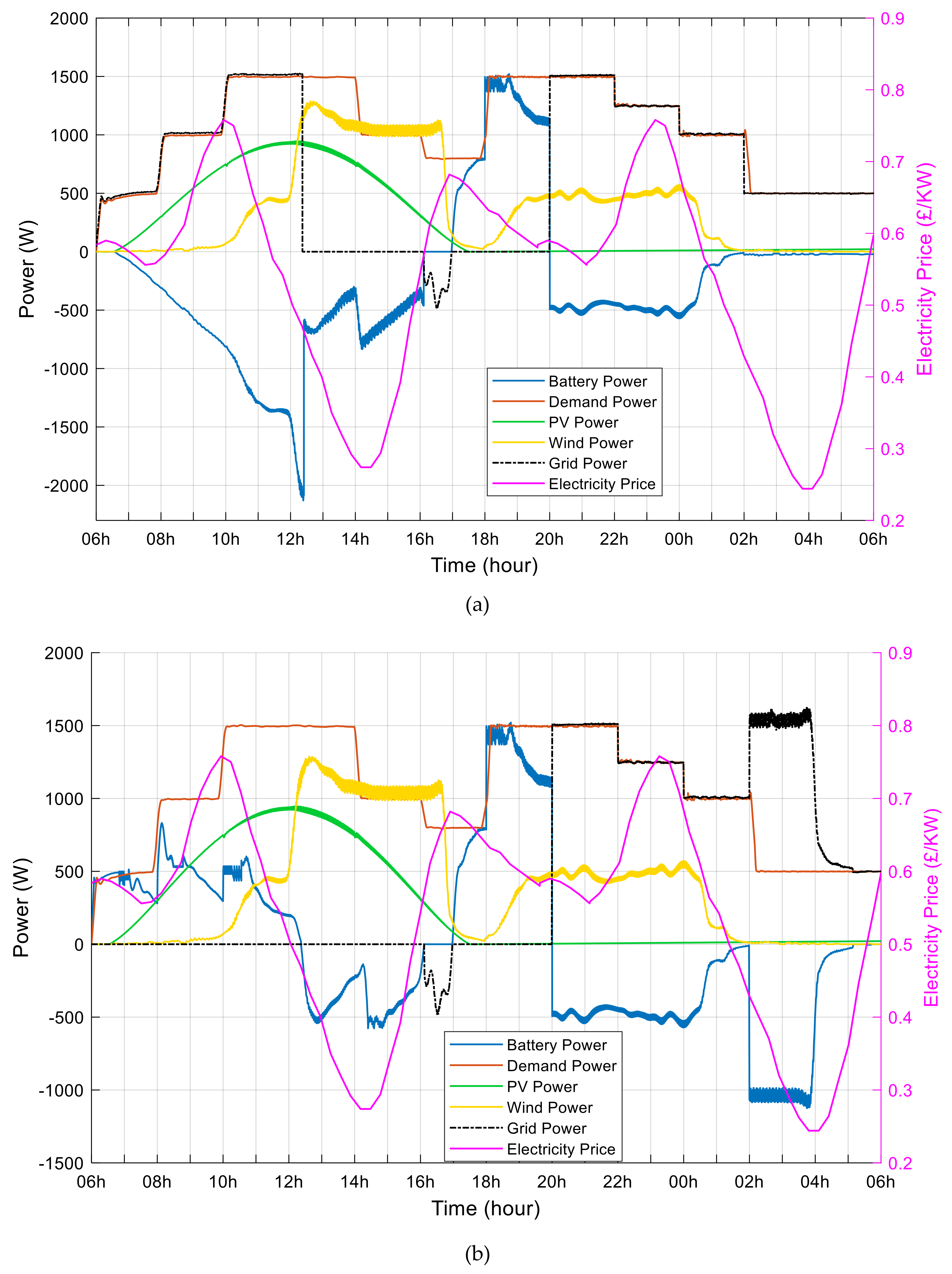
4.1. EM Scenarios Using GPC Control

In the first scenario, a GPC model is integrated to regulate the battery charge/discharge according to the constraints, which are presented by Equation (2) and Equation (13) (i.e., the batteries are initially fully charged). In this scenario, the controller manages the power production/consumption by interacting with the batteries and by performing the actions presented in Figure 5. In this case, batteries are first used to supply the building’s load, especially when the RESs could not satisfy the demand.
The operational behavior of the MG system is depicted in Figure 9. As shown, around 07:00 A.M., the PV panels start to generate the power (green curve), which is accumulated with the batteries’ power (blue curve) in order to ensure the power to the load. Around 08:30 A.M., the wind turbine starts to generate the power (yellow curve) together with the PV and batteries. At 10:00 A.M., the RESs (i.e., PV and wind turbine) generation is becoming higher than the power demand, and the surplus is used to charge the batteries. It is also shown that the GPC-based model took into consideration the objective function (Equation (12)) by keeping, as much as possible, the batteries SoC at its maximum. From 10:00 A.M. to 05:00 P.M., batteries power is again accumulated with the power generated from RESs in order to supply the building’s load, while around 05:00 P.M., the power generated from RESs is almost negligible and, therefore, batteries are the most powerful supplier.
In summary, during this scenario, the MG system is tested in order to show its capability to operate within the variable RESs generation while respecting the above-mentioned constraints, which are incorporated within the GPC-base control model. As demonstrated, without considering the electricity price, the MG system is operated in the autonomous mode and the GPC controller managed efficiently the variable production of RESs by interacting with the storage system. In fact, the proposed GPC model could ensure the island mode detection by managing the power dispatching tasks, which are handled by the secondary layer.
As stated above, the second scenario is mainly dedicated to evaluate the MG system’s behavior when batteries are initially discharged. Since RESs, generations and load demand are considered as measurable disturbances, and only the electricity price is the uncontrollable parameter, the operational behavior MG needs to be adapted, by the GPC-based control, in order to supply the power to building’s load. In this scenario, we consider that the same RESs and loads behaviors are used, but by having the possibility to extract or inject the electricity from or to the utility grid. The GPC controller is designed to manage the switching between batteries and the utility grid without controlling the power, which is generated by RESs. As shown in Figure 10, we consider that RESs are generating the maximum power using the MPPT of the first control layer (green curve for PV generation and yellow curve for wind turbine generation). Under this scenario, the electricity price is taken into account as the main constraint for the tertiary control layer (Equation (17)) for managing the interconnection between the MG system and the utility grid. As defined in Equation (17), the Q 1 matrix elements represent the priority between the RESs, the batteries, and the utility grid for supplying the power to the building’s load while minimizing the cost function, which represents the electricity price variability.
As depicted in Figure 10, the consumption (orange curve) is the set point willing to reach by the GPC model. The aim is to accumulate the RESs power generation, batteries, and the utility grid while minimizing the cost function, which is embedded into the GPC-based control.
At the starting time, the batteries are discharged and the RESs generation is null, therefore the controller uses the utility grid for power supply to the building’s load. As clearly mentioned in Figure 10, from 06:30 A.M. to 10:00 A.M., the RESs generation (green curve) is less than the power demand, consequently, and according to the control diagram of Figure 5, the power generated by RES is only used to charge the batteries. Therefore, the building’s load is completely supplied by the utility grid (black curve). It is worth noting that the operational behavior needs to be avoided in MG systems, as also indicated in Figure 5. More precisely, during this period, the electricity price is higher than the defined threshold value, but the RESs generation is less than the load demand while the batteries are not at the maximum. However, the GPC model could not operate efficiently, since it needs to first satisfy the constraint defined for the secondary control layer while using the RESs power generation in order to charge the batteries, keeping their the SoC at a maximum level.
At 10:00 A.M., the RESs generation is higher than the power demand. In this case, the energy excess is managed according to the electricity price variation. In fact, during the following periods, 10:00 A.M.–11:00 A.M., 02:00 P.M.–03:00 P.M., and 04:00 P.M.–05:00 P.M., the electricity price (pink curve) is higher than the threshold value (red curve). Therefore, the surplus is injected into the utility grid in order to increase the prosumers’ profitability by selling the energy at a high price. From 11:00 A.M. to around 01:00 P.M., the electricity price is less than the threshold value; in this case, instead to inject the surplus into the utility grid, it is used to charge the batteries. Therefore, the batteries are charged and could supply the building’s load, as shown during the period from 03:00 P.M. to around 04:00 P.M.. They are also used for supplying the load even after 05:00 P.M. despite that their SoC is not at the minimum. To summarize, in this second scenario, a fixed threshold value (red curve in Figure 10) of the electricity price is integrated as a cost function for being minimized by the GPC-based control. In fact, the GPC manages the power between the RESs, the batteries, and the utility grid according to the defined priority as well as the constraints for the secondary and the tertiary layers.
Unlike the second scenario, in the third scenario, a dynamic threshold value is used for the electricity price by considering the peak-demand periods. In fact, the electricity price is an interesting exogenous for both prosumers and the utility grid operators. For instance, it could be used by the grid operators as penalties for the consumers, avoiding then the peak-demand. In fact, the consumers can efficiently manage their consumption by using, for example, programmable machines, which could be controlled by integrating “Internet of things” technologies, or by the deployment of intelligent and predictive control strategies. Moreover, in MG systems, the proposed GPC model can locally manage RESs generation and storage devices. For the studied scenario, the electrical grid is used only during some periods, mainly when the electricity price is inexpensive. The batteries’ SoC is kept at its maximum for being used during periods with high electricity price, and consequently, the electricity bill could be minimized. Furthermore, the high electricity demand from the utility grid is minimized avoiding then the generation of peak-demands. As shown in Figure 11, at the starting time, the RESs start charging the batteries and the grid generates the power for supplying the building’s load. From 06:00 A.M. to 08:00 A.M., the MG system operates like in the second scenario. However, during the morning peak-demand period (from 08:00 A.M. to 10:00 A.M.), the electricity price (pink curve) increases to reach the maximum, although the batteries start to generate the electricity to the load in order to avoid using the utility grid, having the highest price. During the periods (from 10:00 A.M. to around 02:00 P.M.), which show the lowest electricity price, the RESs (green curve) supply the power to the load while the surplus is managed in a similar manner as the previous scenario. In the afternoon (from 02:00 P.M. to 04:00 P.M.), there is a peak-demand, as shown by the orange curve (Figure 11). In this period, the surplus generated by RESs is injected into the utility grid while the batteries are used to supply the building’s load (especially when RES generation is low), respecting then, the electricity price variation and the battery SoC constraints.
In summary, from the results, depicted in Figure 11, the deployed GPC model manages the energy flow according to the defined constraints, which are related to the secondary layer (Equation (13)). Moreover, it efficiently handles the cost function related to the tertiary layer (Equation (17)).
The fourth scenario is mainly included to investigate the MG system behavior taking into consideration all constraints defined in Equation (17). The aim is to maximize supplying the building’s load from RESs and batteries, especially when the electricity price is expensive. This priority is selected depending on the elements of the diagonal matrix Q 1 , which are presented in Equation (17). In addition, the action selected by the GPC model, during a given prediction horizon N, considers the variability of electricity price, which is represented by the second term of the Equation (17). Thus, the sources selected to generate the electricity to the loads should be capable to generate the equivalent energy in order to reach the selected set point, presented in the third term of the Equation (17), while the set point is represented by the electricity consumption variability.
In this scenario, the GPC model for EM is deployed during 24 h with the main aim is to show the utility of this model in minimizing the electricity bill. Two cases are considered in order to make a comparative study regarding the electricity cost. For the first case (Case 1), as described in Figure 12a, we have considered a dynamic threshold value for the electricity price, in a similar way as the third scenario. In the second case (Case 2), as depicted in Figure 12b, we consider that the EM system can use the utility grid to charge the batteries, mainly when the electricity price is inexpensive. As already known, batteries are used during the night when the RESs power is unavailable, especially for the PV panels. As shown in Figure 12a, around 05:00 P.M. the RESs generation becomes insignificant (green curve for PV power and yellow curve for the wind power). Consequently, the batteries start generating the power (blue curve) to the loads (orange curve). When the batteries are used, their energy is accumulated with the wind turbine in order to satisfy the requested power.
However, at 08:00 P.M., the batteries’ SoC reached the minimum threshold value (to avoid a deep-discharging) and the wind turbine cannot satisfy alone the energy demand. In this case, the utility grid is used to supply the electricity to the building’s loads, while the power, which is generated by the wind turbine, charges the batteries, from 08:00 P.M. to around 02:00 A.M.. During the rest of the night, the batteries are not fully charged, and, therefore, the load is supplied by the utility grid while the batteries remain at rest. In the morning, starting from 06:00 A.M. to 12:00 A.M., the RESs generation is less than the load’s demand. In this period, as shown in Figure 12a, the power generated by the RESs is entirely stored in the batteries, while the building’s load is supplied by the utility grid. However, from 12:00 A.M. to 04:00 P.M., the RESs generation is higher than the building’s load demand. During this period, and because the electricity price is low, the surplus is then used to charge the batteries. From 04:00 P.M. to 05:00 P.M., the surplus is, however, injected into the utility grid. The aim is to profit from the high electricity price by selling it, and then reducing the electricity bill for consumers. Regarding the second case, as presented in Figure 12b, we consider that the batteries can be charged at night from the utility grid, especially when the electricity price is lower. The system operates like in Case 2. Though, at 02:00 A.M., the utility grid charges the batteries because the electricity price is low and the batteries SoC should be kept at its maximum for being used during the morning in order to avoid the peak-demand. Unlike the first case, the building’s load is supplied, during this peak-demand, only by both the batteries and RESs, without using the utility grid. The main control constraints that are considered in this work is the electricity cost and the battery charge/discharge cycle. In fact, in the presented scenarios, the controller considered the electricity price before switching to the batteries. In this way, at some moments the EM should switch to the batteries because the RESs generation cannot satisfy the demand, but by considering the constraint related to the electricity price and battery charge/discharge cycle minimization, the control strategy uses the utility grid to supply the power to the building’s loads. This decision keeps the batteries fully charged and profits from the low cost of electricity at those moments. As explained above, batteries, as storage devices, are a solution for energy supply only when the constraint of electricity price is not satisfied. In addition, batteries are kept at rest during the night (Figure 12b) to avoid discharging (demi-cycle is minimized) profiting from the low cost of electricity during this period (from 02:00 A.M. to 06:00 A.M.).
To summarize, the above mentioned scenarios focused on the performance evaluation of the GPC-based control for EM in MG systems. We put more emphasis on the operation behavior of the considered MG system following a cost function and the system’s constraints. The next sub-section will focus on the benefit of the GPC-based control on the electricity price.

4.2. The Benefit of GPC Model on the Electricity Price

In this section, the profit of electricity price is computed for the fourth scenario and in both cases (1 and 2, Figure 12), since they represent the entire system’s operations. In this study, the kilowatt-hour is calculated for the power, which is extracted or injected into the utility grid, as well as the power used to charge or discharge the batteries. It is worth noting that the RESs generate the maximum power at each moment without limiting the power by the LPPT (limited power point tracking) algorithms. In the studied scenarios, the possibility to charge the battery from the utility grid was integrated as an important element in the proposed EM strategy for MG systems. However, a high cycle of the batteries’ charge/discharge could play a major role in decreasing the batteries’ state-of-health. The GPC-based control manages the power flow in order to keep, as much as possible, the battery SoC at its maximum (Equation (11)). This avoids a high cycle of charge/discharge and a deep-discharge of batteries, which cause the degradation of their state-of-health.
Regarding Case 1, batteries can only be charged from RESs production. They are mainly used to compensate the power generated for supplying the building’s load according to the constraints, which are set in the deployed GPC-based model. As presented in Table 3 and Table 4, the cost average, the battery power average, and the grid power average are calculated for each hour during the system’s operation period. In fact, the negative average power represents the equivalent power, which is used to charge the batteries, while the positive value is the equivalent power, which is generated from the batteries in order to supply the electricity to the building’s loads.
By comparing this factor in both cases, the batteries have a total battery power-average equal to “−5.71 KWh” and “−0.0042 KWh” respectively for Cases 1 and 2. For Case 1, this is due to the high usage of the utility grid, and consequently, the batteries receive the maximum power from the RESs without considering the electricity price variation, especially during the day. However, in Case 2, the batteries can be charged from the utility grid, mainly when the electricity price is inexpensive. In fact, the negative average of the power grid represents the equivalent power, which is injected to the grid from RESs, while the positive average is equivalent to the power, which is extracted from the grid in order to satisfy the load demand. As depicted in Table 3, in Case 1, “15.36 KWh” of energy is used from the utility grid, representing an equivalent of “8.97 €” for 24 h, while in Case 2, only “11.42 KWh” of energy is extracted from the grid, which is equivalent to “5.85 €” for the same period.
Therefore, different factors are considered in order to manage the energy flow in the MG system. In order to maximize its profitability, for all studied scenarios, the RESs generate, at each moment, the maximum power. When RESs cannot satisfy the demand, the grid and the batteries’ power are efficiently managed in order to avoid the degradation of batteries state-of-health, while minimizing the electricity bill. In summary, the above-mentioned results show the usefulness of the GPC-based control in minimizing the electricity bill by integrating the electricity price as a main important factor for EM in MG systems. However, the power quality as well as the timely decision, which is provided by the GPC-base control, has to be assessed. The next sub-section focuses on evaluating and assessing these two important factors.
For the real deployment and testing of the proposed control strategy, a real platform is ongoing development. The proposed platform uses the new information and communication technologies to improve the performance of the GPC controller. The deployed platform contains RESs and battery storage systems, which are connected together with the TEG in order to supply the electrical energy to the building’s loads (e.g., lighting, ventilation) as is mentioned in Figure 13. The IoT/big data platform was developed and deployed in order to allow measuring and forecasting RESs power generation, loads consumption, and batteries SoC. Sensing/actuating components with a control card are installed in order to monitor and manage the whole MG system offering the possibility to test the developed control techniques in the real context. The deployed sensors are used to collect the control input parameters (e.g., power demand, power production, SoC), which is sent by a micro-computer (Raspberry-pi) to a deployed cluster that present a preferment calculation node. Due to the limited calculation performances of the actual inverters, it is planned to propose an IoT architecture that integrate the inverter as a device in the MG system that can communicate with the whole other devices (consumers, producers). The measurements will be sent to a cluster to execute the control algorithm and to calculate the optimal control actions that will be resubmitted to the local inverter for execution. In addition, machine-learning algorithms can be deployed to forecast the control input parameters and the disturbances events that can influence the control decision in the MG. The actual inverters have the possibility to be connected to the internet to store the data, for that the idea is use to use this data to increase the performances of the inverter by integrating more sophisticated control algorithms with variable constraints, cost function, and optimization methods.

4.3. State of the Art Synthesis and Our Contribution

Control strategies, generally, use single-objective function procedures (e.g., maximizing the quality of the services). Without considering different operating constraints, these procedures are easier to implement and to deploy in real-sitting scenarios. Moreover, control strategies, which take into consideration only the energy availability within MG components (e.g., energy sources, storage devices, traditional electric grid), could be implemented by simple algorithms. These algorithms implement procedures that switch, at each time, from RES to either storage devices or to the TEG. For instance, actual commercial inverters are able to manage efficiently the interconnection between RESs, energy storage systems, and the utility grid by incorporating a single-objective function. In particular, the MG system’s EM takes into consideration only the availability of the electricity for being supplied to buildings loads. The inverter can use once either batteries or the utility grid without taking into account other parameters, such as the actual electricity cost as well as batteries’ charge/discharge cycles. However, high batteries’ charge/discharge cycles, in a limited time, could decrease their performances, which impact the profitability of the system. In other cases, controllers can interact, in real-time, with energy sources generators (e.g., solar, wind) in order to limit the power generation (limited power point tracking). The aim is to ensure the quality of the electrical services (e.g., frequency, voltage), and consequently minimizing the profitability of the MG system’s components. Despite their advantages, they could have, however, negative impacts on the batteries’ lifecycle and system’s profitability. Therefore, context-awareness principles and predictive analytics could be exploited for developing context-driven control approaches.
This work contribution to the current state of knowledge aims to develop context-driven control approaches for EM of MG systems in the context of smart buildings. Unlike the control approaches from literature, the proposed strategy considers multiple objectives functions, which take into consideration batteries charge/discharge cycles as well as the electricity price forecasting. The main aim is to ensure, in an optimal way, the continuous electricity supply from different installed sources (e.g., RESs, batteries, TEG) to the building’s services. The proposed approach is based on predictive control models, which are able to generate a sequence of future control actions over a prediction horizon based on the MAPCASTE (measure, analyze, plan, forecast, and execute) approach (Figure 14). The obtained results show the usefulness of the proposed control strategy to minimize the electricity price for the consumer.
However, in order to carry out the control approach, several forecasted inputs values are required, mainly the power production/consumption and batteries SoC. This requires an advanced metering infrastructure, which allows measuring and predicting all input values in order to enhance the GPC performances.

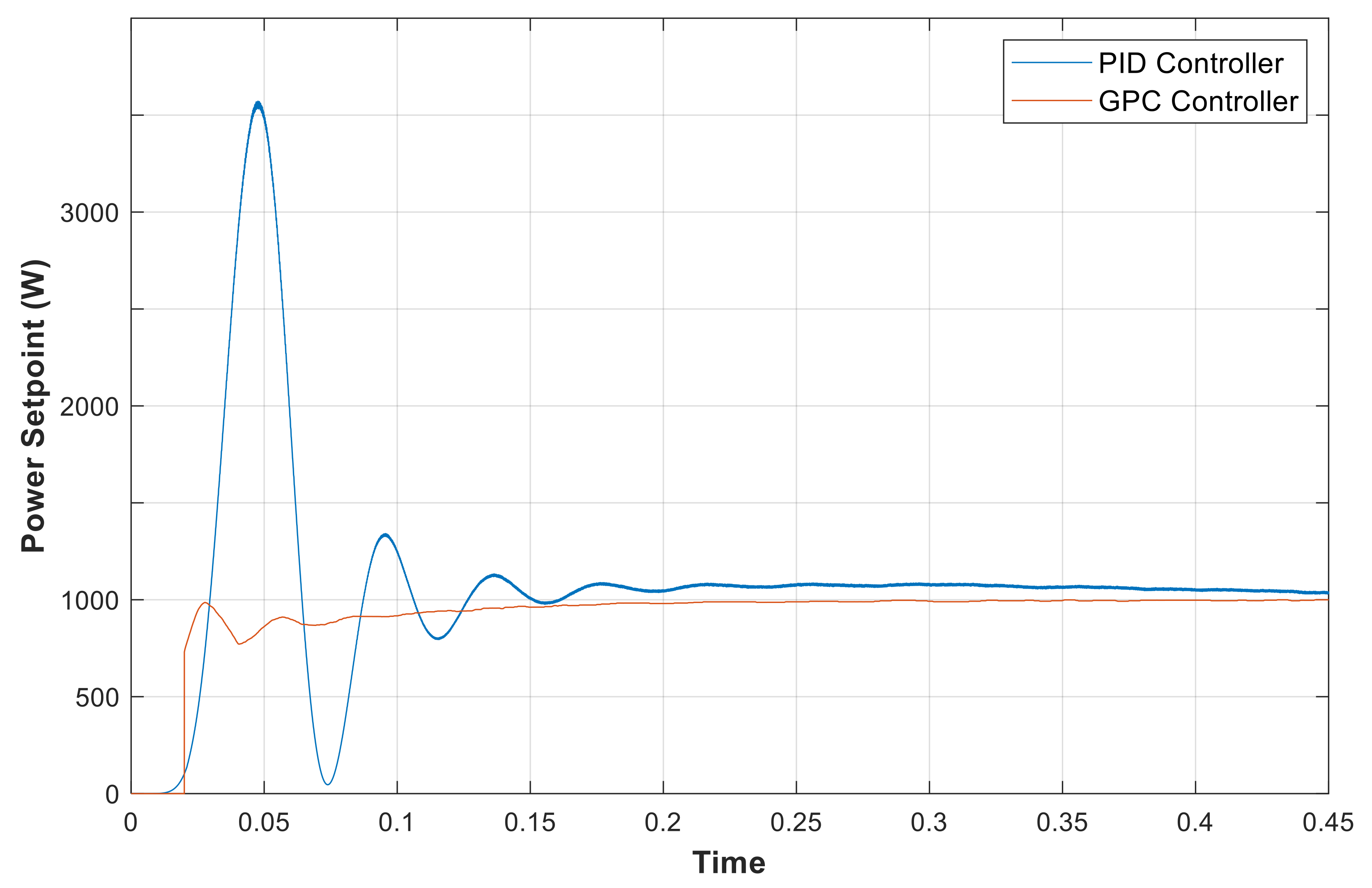
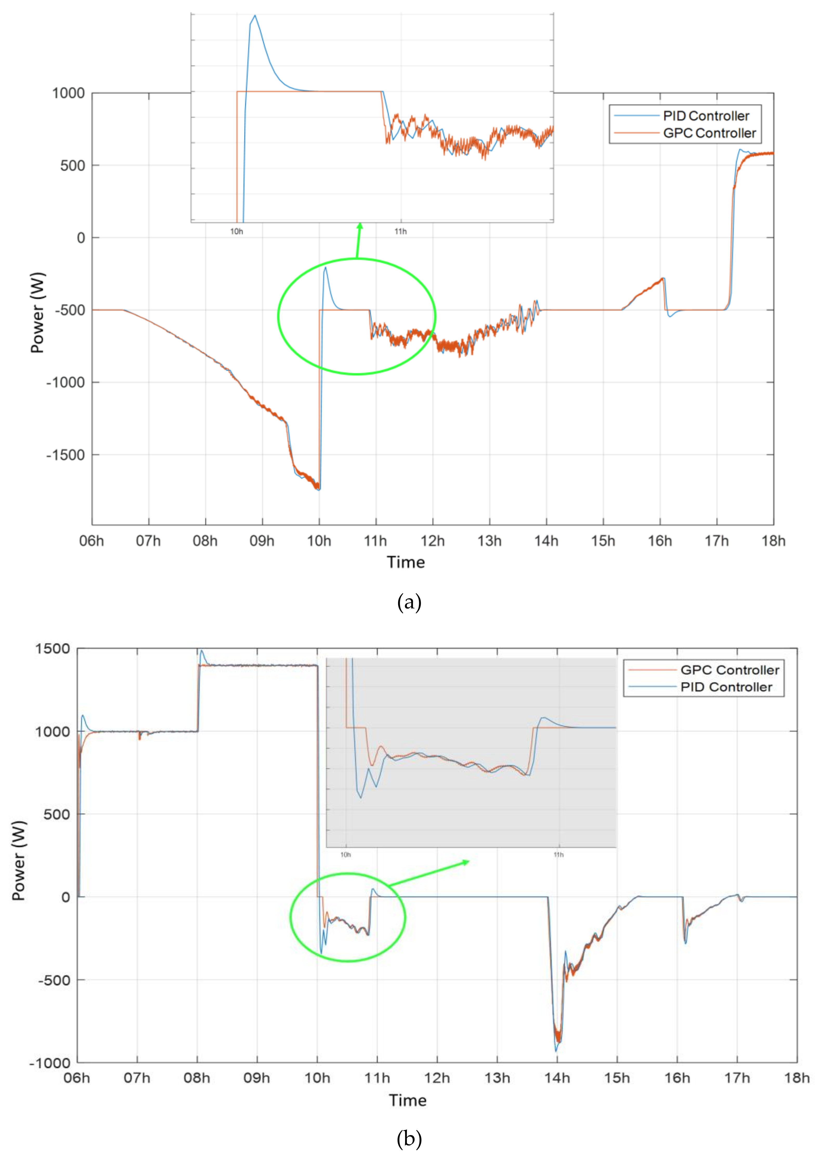
4.4. GPC Controller for Power Quality Regulation

Computing and data processing, for providing timely decisions and actions, are of most importance, especially in systems requiring real-time predictive control. For instance, as stated above, a delay is created between the measurement time and the application of the predicted control action. In fact, between two moments ( t k and t k + 1 ), the previous state continues to control the system, and consequently, the voltage vector, selected at time t k , continues to be applied after t k + 1 . This makes the power oscillates around the reference, and then the “current ripple” increases. Therefore, by using the GPC controller for the tertiary control layer, the predictor calculates, for each instant t k , the predictions of the dynamic evolution of the process y t + 1 ,   ,   y t + N T , throughout the prediction horizon N . This prediction is based on dynamic parameters, which are measured at this moment, as well as on future control regulations u t ,   u t + 1 ,   ,   u t + N T , along the prediction horizon N . As depicted in Figure 15, the orange curve represents the output power, which is generated by the inverter according to the GPC-based control, while the blue curve represents the power, which is generated by the inverter according to a PID (proportional–integral–derivative) controller. As shown in Figure 15, unlike the PID controller, which takes a few moments to reach the set point regulation (1000 W of load consumption), the GPC controller generates the future control actions by keeping the system’s output as close as possible to the set point. In fact, the GPC controller shows more system’s stability during the switching moments.
For the PID, a simple setting is realized with the main focus is the development of a predictive controller, which is based on data prediction and forecast to generate suitable action for EM [3]. In this comparison scenario, the controller is used in a closed-loop unity feedback system. The tracking error e is sent to the PID controller and the generated control signal u t from the controller to the inverter is equal to the proportional gain ( K p ) times the magnitude of the error plus the integral gain ( K i ) times the integral of the error plus the derivative gain ( K d ) times the derivative of the error.
u = K p . e + K i . e . d t + K d . d e d t
Based on the control action (Equation (31)) generated from the controller PID, the K p regulation decreases the rise time, the K i eliminates the steady-state error, and the K d reduces the overshot and settling time. The PID can operate with high performance for real-time data processing using the system “feedback” as the main element for the model stability. However, the predictive control uses the system “feedforward” that can interact with the system’s output before the command execution. Unlike the PID, the predictive control/command offers the possibility to integrate multiple objective functions and control constraints. For obtaining accurate values of K p , K i , and K d , the Sisotool in MATLAB/SIMULINK can be used. In this simple study, the PID is tuned for K p = 2.75 , K i = 0.984 , and K d = 1.73 . Since the voltage loop and current loop are decoupled, each PID controller can be designed separately. Therefore, for Figure 15, the presented peak for the PID control, at the switching moments, can be adjusted by regulating the PID coefficients and it is enlarged to show this existing issue with the PID controller compared to the GPC controller. For the PID, the DC link capacitor output voltage presented an overshoot (generating an overshoot of power) and the GPC controller gives less overshoot. It is also observed from the result that the inductor current achieves its steady state value faster with the GPC controller.
Moreover, the control strategy decision by the GPC-based control is mainly generated for the secondary and tertiary control layer. In fact, the GPC manages the system for the secondary control layer by taking the right action on batteries charge/discharge according to the detected mode, autonomous grid-connected. As shown in Figure 16, the PID controller takes more time to converge to the desired references, especially during switching moments. Since the PID is based on a feedback control mechanism (i.e., cannot generate future actions) and the studied constraints cannot be modeled for real-time control, we present only the result when the PID is applied for the grid-connected mode with a static set point. Unlike PID, the GPC controller is based on a feed-forward control mechanism, which allows it to generate future actions according to a predefined cost function and constraints. As depicted in Figure 16a, the regulation of batteries charge/discharge decision is more stable at the switching moments and without a significant “current ripple”. Similarly, high switching performance are presented for the interconnection with the electrical grid (Figure 16b). This is due to the delay compensation method, which is used by the GPC-based control.
Furthermore, the GPC model gives an exact solution to an approximated optimization problem by calculating the voltage reference to the inverter. However, this voltage is generated by a PWM (pulse width modulation) or SVM (space vector modulation) technique. As presented in Figure 6, the power circuit of a grid-connected converter is represented by a smoothing inductor. The main objective of the GPC model is to calculate, for the inverter, the reference of the output voltage for each connected source and load or injection of power to the grid. For the controller, the main variables are the DC voltage/current, the grid voltage/current, and the load voltage/current. The inverter should be able to regulate the output depending on the parameter variation of the DC bus. The output of the system is modeled by Equation (30), in which the output voltage and current are regulated following the references that are generated by the GPC-based control. Figure 17 presents the obtained regulation of voltage and current for the deployed power converter depending on the DC voltage variation. Figure 17a–c show respectively the DC voltage, the DC current, and the current across the LC filter capacitor.
The active power filter consists essentially of a voltage source inverter and a DC bus, which is connected to a capacitor, while the AC bus is connected to the main grid through an LC filter. Mainly, for each load connected to the AC bus, the converter should be capable to generate the suitable current and voltage. For the studied scenarios, the voltage and frequency of the grid are set as 240 V and 50 Hz, respectively. Depending on the deployed loads used for our scenarios, Figure 18a presents the current variation and Figure 18b presents the voltage, which are measured at the output of the inverter.
The frequency spectrum is presented for the AC bus voltage and current and for the load voltage as shown in Figure 19. Depending on the Equation (25) dynamics, the voltage-source-inverter output is chosen as the control signal and the final switching sequence is generated through a PWM technique. The performance is analyzed for an RLC load, which is deployed for simulation purposes. Thus, the converter must ensure the stability of the energy injected into the utility grid, according to the rules established by the operators [56].
It is worth noting that, in power electronics, the state feedback regulators do not guarantee a good performance in terms of rapid recovery and low harmonic distortion of the output, especially when the system is affected by disturbances and variations in parameters. However, the use of a feed-forward technique improves the transient response and minimizes, even remove harmonic disturbances. Better performance of this type of controllers is achieved, as shown in Figure 19. The output tracks the reference voltage and current with good behavior by ensuring the stability of the system’s frequency at 50 Hz for harmonic loads. Furthermore, the GPC provides an explicit solution for unconstrained predictive control. It is also able to handle the problem of mismatch between the model and the deployed load.

5. Conclusions and Perspectives

In this paper, an energy management system, based on a generalized predictive control approach, was introduced for being deployed in the secondary and the tertiary control layers. In fact, the secondary layer focused on power regulation and energy demand/response balance. An optimization function was defined, for this level, by considering a GPC strategy. State-space equations are presented for the controllable micro-grid system’s entities depending on the constraint, which is defined in the tertiary control layer. Therefore, the tertiary control focused only on power dispatch and economic aspects. Within this context, the electricity cost is used as a constraint to control the batteries charge/discharge. Indeed, the electricity price is integrated as a cost function to be minimized while respecting the constraint defined by the GPC model. The controller manages the power between the RESs, the batteries, and the utility grid depending on the operational constraints of the EM strategy deployed using the GPC model. The powerful of the GPC model for the EM system was shown by minimizing the electricity bill. For a given scenario, the deployed control strategy manages the energy flow in the deployed MG system depending on the electricity price variability during the day. The main objective is to ensure the power to the consumer with a minimum price by integrating predictive control methods that considers multiple objective function and constraint. While the battery charge/discharge current is controlled depending on the defined constraint with the possibility to charge the battery storage system from the utility grid when the electricity price is minimal. It is worth noting that actual controllers of the power converter manage the energy flow based on real-time measurement (e.g., current, voltage, power), however, it is possible to control the power exchange using predictive control offering the possibility to integrate multi-objective functions and constraints. Today, it is possible to connect actual inverters with the Internet in order to store, process, and analyze measured data. These latter could be used to train machine learning algorithms and to generate the control input parameters offering more accuracy for the predictive control. In future works, a power converter will be deployed based on the GPC controller for energy management in our actual MG system.

Author Contributions

Conceptualization, A.E., M.B. and R.O.; data curation, A.E.; methodology, A.E., R.O. and M.B.; software, A.E. and R.O.; supervision, R.O., M.B., N.E.k. and K.Z.-D.; validation, R.O. and M.B.; writing—original draft, A.E.; writing—review and editing, A.E., M.B., N.E.k. and K.Z.-D. All authors have read and agreed to the published version of the manuscript.

Funding

This work is supported by IRESEN-Innov-Project (2020–2022), under the HOLSYS project program. It is also partially supported by MIGRID project (Grant 5-398, 2017–2019), which is funded by USAID under the PEER program.

Data Availability Statement

Data sharing is not applicable to this article.

Conflicts of Interest

The authors declare no conflict of interest. The funders and the project participants had no role in the design of the study; in the collection, analyses, or interpretation of data; in the writing of the manuscript, or in the decision to publish the results.

References

  1. Elmouatamid, A.; NaitMalek, Y.; Ouladsine, R.; Bakhouya, M.; Elkamoun, N.; Khaidar, M.; Zine-Dine, K. A Micro-grid system infrastructure for efficient energy management in smart buildings. In Submitted to ATSPES’1 (Advanced Technologies for Solar Photovoltaics Energy Systems); Springer: Cham, Switzerland, 2020. [Google Scholar]
  2. Li, J.; Murphy, E.; Winnick, J.; Kohl, P.A. Studies on the cycle life of commercial lithium-ion batteries during rapid charge–discharge cycling. J. Power Sources 2001, 102, 294–301. [Google Scholar] [CrossRef]
  3. Elmouatamid, A. MAPCAST: An adaptive control approach using predictive analytics for energy balance in micro-grid systems. Int. J. Renew. Energy Res. 2020, 10, 945–954. [Google Scholar]
  4. Elmouatamid, A.; NaitMalek, Y.; Bakhouya, M.; Ouladsine, R.; Elkamoun, N.; Zine-Dine, K.; Khaidar, M. An energy management platform for micro-grid systems using internet of things and big-data technologies. Proc. Inst. Mech. Eng. Part I J. Syst. Control. Eng. 2019, 233, 904–917. [Google Scholar] [CrossRef]
  5. Elmouatamid, A.; Ouladsine, R.; Bakhouya, M.; Zine-Dine, K.; Khaidar, M. A Control Strategy Based on Power Forecasting for Micro-Grid Systems. In Proceedings of the 2019 IEEE International Smart Cities Conference (ISC2), Casablanca, Morocco, 14–17 October 2019; pp. 735–740. [Google Scholar]
  6. Serale, G.; Fiorentini, M.; Capozzoli, A.; Bernardini, D.; Bemporad, A. Model predictive control (MPC) for enhancing building and HVAC system energy efficiency: Problem formulation, applications and opportunities. Energies 2018, 11, 631. [Google Scholar] [CrossRef] [Green Version]
  7. Elkhoukhi, H.; NaitMalek, Y.; Bakhouya, M.; Berouine, A.; Kharbouch, A.; Lachhab, F.; Essaaidi, M. A platform architecture for occupancy detection using stream processing and machine learning approaches. Concurr. Comput. Pract. Exp. 2020, 32, e5651. [Google Scholar] [CrossRef]
  8. NaitMalek, Y.; Najib, M.; Bakhouya, M.; Essaaidi, M. On the Use of Machine Learning for State-of-Charge Forecasting in Electric Vehicles. In Proceedings of the 2019 IEEE International Smart Cities Conference (ISC2), Casablanca, Morocco, 14–17 October 2019; pp. 408–413. [Google Scholar]
  9. Elmouatamid, A.; Ouladsine, R.; Bakhouya, M.; El Kamoun, N.; Khaidar, M.; Zine-Dine, K. Review of control and energy management approaches in micro-grid systems. Energies 2020, 14, 168. [Google Scholar] [CrossRef]
  10. Hu, J.; Zhu, J.; Guerrero, J.M. Model Predictive Control of Smart Microgrids. In Proceedings of the 2014 17th International Conference on Electrical Machines and Systems (ICEMS), Hangzhou, China, 22–25 October 2014; pp. 2815–2820. [Google Scholar]
  11. Dehghani-Pilehvarani, A.; Markou, A.; Ferrarini, L. A hierarchical distributed predictive control approach for microgrids energy management. Sustain. Cities Soc. 2019, 48, 101536. [Google Scholar]
  12. Marzband, M.; Yousefnejad, E.; Sumper, A.; Domínguez-García, J.L. Real time experimental implementation of optimum energy management system in standalone microgrid by using multi-layer ant colony optimization. Int. J. Electr. Power Energy Syst. 2016, 75, 265–274. [Google Scholar] [CrossRef] [Green Version]
  13. Elmouatamid, A.; Ouladsine, R.; Bakhouya, M.; El Kamoun, N.; Zine-Dine, K.; Khaidar, M. A Model Predictive Control Approach for Energy Management in Micro-Grid Systems. In Proceedings of the 2019 International Conference on Smart Energy Systems and Technologies (SEST), Porto, Portugal, 9–11 September 2019; pp. 1–6. [Google Scholar]
  14. Hosseinzadeh, M.; Salmasi, F.R. Robust optimal power management system for a hybrid AC/DC micro-grid. IEEE Trans. Sustain. Energy 2015, 6, 675–687. [Google Scholar] [CrossRef]
  15. Luna, A.C.; Diaz, N.L.; Graells, M.; Vasquez, J.C.; Guerrero, J.M. Mixed-integer-linear-programming-based energy management system for hybrid PV-wind-battery microgrids: Modeling, design, and experimental verification. IEEE Trans. Power Electron. 2017, 32, 2769–2783. [Google Scholar] [CrossRef] [Green Version]
  16. Vergara, P.P.; López, J.C.; da Silva, L.C.; Rider, M.J. Security-constrained optimal energy management system for three-phase residential microgrids. Electr. Power Syst. Res. 2017, 146, 371–382. [Google Scholar] [CrossRef]
  17. Xiang, Y.; Liu, J.; Liu, Y. Robust energy management of microgrid with uncertain renewable generation and load. IEEE Trans. Smart Grid 2015, 7, 1034–1043. [Google Scholar] [CrossRef]
  18. Berouine, A.; Ouladsine, R.; Bakhouya, M.; Essaaidi, M. Towards a real-time predictive management approach of indoor air quality in energy-efficient buildings. Energies 2020, 13, 3246. [Google Scholar] [CrossRef]
  19. Buyak, N.A.; Deshko, V.I.; Sukhodub, I.O. Buildings energy use and human thermal comfort according to energy and exergy approach. Energy Build. 2017, 146, 172–181. [Google Scholar] [CrossRef]
  20. Rahmani-Andebili, M.; Shen, H. Cooperative Distributed Energy Scheduling for Smart Homes Applying Stochastic Model Predictive Control. In Proceedings of the 2017 IEEE International Conference on Communications (ICC), Paris, France, 21–25 May 2017; pp. 1–6. [Google Scholar]
  21. Hemmati, R.; Saboori, H. Stochastic optimal battery storage sizing and scheduling in home energy management systems equipped with solar photovoltaic panels. Energy Build. 2017, 152, 290–300. [Google Scholar] [CrossRef]
  22. Bordons, C.; Teno, G.; Marquez, J.J.; Ridao, M.A. Effect of the Integration of Disturbances Prediction in Energy Management Systems for Microgrids. In Proceedings of the 2019 International Conference on Smart Energy Systems and Technologies (SEST), Porto, Portugal, 9–11 September 2019; pp. 1–6. [Google Scholar]
  23. Petrollese, M. Optimal Generation Scheduling for Renewable Microgrids Using Hydrogen Storage Systems. Ph.D. Thesis, The University of Cagliari, Cagliari, Italy, 2015. [Google Scholar]
  24. Negenborn, R.R.; Houwing, M.; De Schutter, B.; Hellendoorn, J. Model Predictive Control for Residential Energy Resources Using a Mixed-Logical Dynamic Model. In Proceedings of the 2009 International Conference on Networking, Sensing and Control, Okayama, Japan, 26–29 March 2009; pp. 702–707. [Google Scholar]
  25. Mendes, P.R.; Isorna, L.V.; Bordons, C.; Normey-Rico, J.E. Energy management of an experimental microgrid coupled to a V2G system. J. Power Sources 2016, 327, 702–713. [Google Scholar] [CrossRef]
  26. Garcia-Torres, F.; Vilaplana, D.G.; Bordons, C.; Roncero-Sanchez, P.; Ridao, M.A. Optimal management of microgrids with external agents including battery/fuel cell electric vehicles. IEEE Trans. Smart Grid 2018, 10, 4299–4308. [Google Scholar] [CrossRef]
  27. Chen, H.; Chen, J.; Lu, H.; Yan, C.; Liu, Z. A modified MPC-based optimal strategy of power management for fuel cell hybrid vehicles. IEEE/ASME Trans. Mechatron. 2020, 25, 2009–2018. [Google Scholar] [CrossRef]
  28. Parisio, A.; Rikos, E.; Tzamalis, G.; Glielmo, L. Use of model predictive control for experimental microgrid optimization. Appl. Energy 2014, 115, 37–46. [Google Scholar] [CrossRef]
  29. Bozchalui, M.C.; Hashmi, S.A.; Hassen, H.; Canizares, C.A.; Bhattacharya, K. Optimal operation of residential energy hubs in smart grids. IEEE Trans. Smart Grid 2012, 3, 1755–1766. [Google Scholar] [CrossRef]
  30. Garcia-Torres, F.; Vazquez, S.; Moreno-Garcia, I.M.; Gil-de-Castro, A.; Roncero-Sanchez, P.; Moreno-Munoz, A. Microgrids power quality enhancement using model predictive control. Electronics 2021, 10, 328. [Google Scholar] [CrossRef]
  31. Bordons, C.; Montero, C. Basic principles of MPC for power converters: Bridging the gap between theory and practice. IEEE Ind. Electron. Mag. 2015, 9, 31–43. [Google Scholar] [CrossRef]
  32. Linder, A.; Kennel, R. Model Predictive Control for Electrical Drives. In Proceedings of the 2005 IEEE 36th Power Electronics Specialists Conference, Dresden, Germany, 16 June 2005; pp. 1793–1799. [Google Scholar]
  33. Rodriguez, J.; Pontt, J.; Silva, C.A.; Correa, P.; Lezana, P.; Cortés, P.; Ammann, U. Predictive current control of a voltage source inverter. IEEE Trans. Ind. Electron. 2007, 54, 495–503. [Google Scholar] [CrossRef]
  34. Gregor, R.; Barrero, F.; Toral, S.; Arahal, M.R.; Prieto, J.; Durán, M.J. Enhanced Predictive Current Control Method for the Asymmetrical Dual—Three Phase Induction Machine. In Proceedings of the 2009 IEEE International Electric Machines and Drives Conference, Miami, FL, USA, 3–6 May 2009; pp. 265–272. [Google Scholar]
  35. Cortes, P.; Wilson, A.; Kouro, S.; Rodriguez, J.; Abu-Rub, H. Model predictive control of multilevel cascaded H-bridge inverters. IEEE Trans. Ind. Electron. 2010, 57, 2691–2699. [Google Scholar] [CrossRef]
  36. Lezana, P.; Aguilera, R.; Quevedo, D.E. Model predictive control of an asymmetric flying capacitor converter. IEEE Trans. Ind. Electron. 2008, 56, 1839–1846. [Google Scholar] [CrossRef]
  37. Vargas, R.; Ammann, U.; Hudoffsky, B.; Rodriguez, J.; Wheeler, P. Predictive torque control of an induction machine fed by a matrix converter with reactive input power control. IEEE Trans. Power Electron. 2010, 25, 1426–1438. [Google Scholar] [CrossRef]
  38. Correa, P.; Rodríguez, J.; Rivera, M.; Espinoza, J.R.; Kolar, J.W. Predictive control of an indirect matrix converter. IEEE Trans. Ind. Electron. 2009, 56, 1847–1853. [Google Scholar] [CrossRef]
  39. Vazquez, S.; Leon, J.I.; Franquelo, L.G.; Rodriguez, J.; Young, H.A.; Marquez, A.; Zanchetta, P. Model predictive control: A review of its applications in power electronics. IEEE Ind. Electron. Mag. 2014, 8, 16–31. [Google Scholar] [CrossRef]
  40. Fontenot, H.; Dong, B. Modeling and control of building-integrated microgrids for optimal energy management—A review. Appl. Energy 2019, 254, 113689. [Google Scholar] [CrossRef]
  41. Villalón, A.; Rivera, M.; Salgueiro, Y.; Muñoz, J.; Dragičević, T.; Blaabjerg, F. Predictive control for microgrid applications: A review study. Energies 2020, 13, 2454. [Google Scholar] [CrossRef]
  42. Hu, J.; Shan, Y.; Guerrero, J.M.; Ioinovici, A.; Chan, K.W.; Rodriguez, J. Model predictive control of microgrids–An overview. Renew. Sustain. Energy Rev. 2021, 136, 110422. [Google Scholar] [CrossRef]
  43. Jayachandran, M.; Ravi, G. Decentralized model predictive hierarchical control strategy for islanded AC microgrids. Electr. Power Syst. Res. 2019, 170, 92–100. [Google Scholar] [CrossRef]
  44. Tedesco, F.; Mariam, L.; Basu, M.; Casavola, A.; Conlon, M.F. Economic model predictive control-based strategies for cost-effective supervision of community microgrids considering battery lifetime. IEEE J. Emerg. Sel. Top. Power Electron. 2015, 3, 1067–1077. [Google Scholar] [CrossRef]
  45. Drgoňa, J.; Arroyo, J.; Figueroa, I.C.; Blum, D.; Arendt, K.; Kim, D.; Helsen, L. All you need to know about model predictive control for buildings. Annu. Rev. Control. 2020, 50, 190–232. [Google Scholar] [CrossRef]
  46. Ławryńczuk, M. Computationally Efficient Model Predictive Control Algorithms; Springer: Berlin, Germany, 2014. [Google Scholar]
  47. Lv, J.; Wang, X.; Wang, G.; Song, Y. Research on control strategy of isolated DC microgrid based on SOC of energy storage system. Electronics 2021, 10, 834. [Google Scholar] [CrossRef]
  48. Grigg, C.; Wong, P.; Albrecht, P.; Allan, R.; Bhavaraju, M.; Billinton, R.; Li, W. The IEEE reliability test system-1996. A report prepared by the reliability test system task force of the application of probability methods subcommittee. IEEE Trans. Power Syst. 1999, 14, 1010–1020. [Google Scholar] [CrossRef]
  49. Clarke, D.W.; Mohtadi, C. Properties of generalized predictive control. Automatica 1989, 25, 859–875. [Google Scholar] [CrossRef]
  50. Yi, X.; Zhang, J.; Wang, Z.; Li, T.; Zheng, Y. Deep Distributed Fusion Network for Air Quality Prediction. In Proceedings of the 24th ACM SIGKDD International Conference on Knowledge Discovery & Data Mining, London, UK, 19–23 August 2018; pp. 965–973. [Google Scholar] [CrossRef]
  51. Bruninx, K.; Delarue, E. A statistical description of the error on wind power forecasts for probabilistic reserve sizing. IEEE Trans. Sustain. Energy 2014, 5, 995–1002. [Google Scholar] [CrossRef]
  52. Camacho, E.F.; Alba, C.B. Model Predictive Control; Springer Science & Business Media: London, UK, 2013. [Google Scholar]
  53. Vazquez, S.; Rodriguez, J.; Rivera, M.; Franquelo, L.G.; Norambuena, M. Model predictive control for power converters and drives: Advances and trends. IEEE Trans. Ind. Electron. 2016, 64, 935–947. [Google Scholar] [CrossRef] [Green Version]
  54. Cortes, P.; Rodriguez, J.; Silva, C.; Flores, A. Delay compensation in model predictive current control of a three-phase inverter. IEEE Trans. Ind. Electron. 2011, 59, 1323–1325. [Google Scholar] [CrossRef]
  55. Larrinaga, S.A.; Vidal, M.A.R.; Oyarbide, E.; Apraiz, J.R.T. Predictive control strategy for DC/AC converters based on direct power control. IEEE Trans. Ind. Electron. 2007, 54, 1261–1271. [Google Scholar] [CrossRef]
  56. IEEE Standard Association. Standard for Interconnection and Interoperability of Distributed Energy Resources with Associated Electric Power Systems Interfaces; IEEE Standard Association: Piscataway, NJ, USA, 2018; pp. 1547–2018. [Google Scholar] [CrossRef]
Figure 1. Energy management schemes with GPC operation processes (Reprinted from ref. [3]).
Electronics 10 01666 g001
Figure 2. Micro-grid energy management levels.
Electronics 10 01666 g002
Figure 3. Hierarchical control levels.
Electronics 10 01666 g003
Figure 4. A schematic view of GPC concept: (a) control actions on the horizon N, (b) predictive control mechanism.
Electronics 10 01666 g004
Figure 5. Energy management and control strategy.
Electronics 10 01666 g005
Figure 6. (a) Single-phase MG system, (b) the test system with one-line diagram.
Electronics 10 01666 g006
Figure 7. Predictive control operation, (a) ideal case: calculation time is negligible, (b) practical case: calculation time is significant.
Electronics 10 01666 g007
Figure 8. Predictive control with significant calculation time: operation of delay compensation method.
Electronics 10 01666 g008
Figure 9. GPC control for autonomous operation mode.
Electronics 10 01666 g009
Figure 10. Energy management scenarios based on GPC model controller for the grid-connected mode and static set point.
Electronics 10 01666 g010
Figure 11. GPC controller for the grid-connected mode and dynamic set point.
Electronics 10 01666 g011
Figure 12. Energy management scenarios based on GPC model, (a) Case 1: without battery-grid interaction, (b) Case 2: with battery-grid interaction.
Electronics 10 01666 g012
Figure 13. Data monitoring platform for energy management and GPC controller deployment.
Electronics 10 01666 g013
Figure 14. The proposed control approach schemes with operation process.
Electronics 10 01666 g014
Figure 15. Power regulation for the GPC and PID controller.
Electronics 10 01666 g015
Figure 16. Power regulation for GPC and PID controller, (a) battery power regulation, (b) grid power exchange.
Electronics 10 01666 g016
Figure 17. Current and voltage regulation, (a) DC bus voltage, (b) DC bus current, (c) the current across the filter capacitor.
Electronics 10 01666 g017
Figure 18. (a) Load current variation, (b) load voltage variation.
Electronics 10 01666 g018
Figure 19. Frequency spectrum, (a) inverter output current, (b) inverter output voltage, (c) load voltage.
Electronics 10 01666 g019aElectronics 10 01666 g019b
Table 1. GPC algorithms’ input parameters.
Input ParametersControl Horizon ( N u )Prediction Horizon ( N p )Sampling Time ( T s )Weighting Control ( λ )
Value41010 s0.6
Table 2. MG system parameters.
DescriptionValue
DC bus voltage320 V
Grid Nominal voltage240 V
System Nominal frequency50 Hz
DC link capacitance2.2 μF
LC Filter inductance0.4 μH
LC Filter capacitance6.85 μF
VSC rated power3 KW
Load capacitance100 mH
Load inductance1 pF
PWM carrier frequency10 KHz
Sampling frequency5 KHz
Battery capacity150 Ah
Maximum PV power1 KW
Maximum wind power1.5 KW
Table 3. Electricity price benefit for Case 1.
BatteryGrid
Time *Cost Average (€)Power Average (KWh)Power Average (KWh)Equivalent Cost Exchange
06 h–07 h0.58−0.020.410.24
07 h–08 h0.56−0.190.500.28
08 h–09 h0.6−0.440.980.59
09 h–10 h0.72−0.691.000.73
10 h–11 h0.70−1.051.481.05
11 h–12 h0.57−1.351.480.84
12 h–13 h0.45−1.130.540.25
13 h–14 h0.33−0.4600
14 h–15 h0.28−0.6700
15 h–16 h0.43−0.4700
16 h–17 h0.63−0.04−0.28−0.18
17 h–18 h0.66−0.6500
18 h–19 h0.62−1.4200
19 h–20 h0.59−1.1700
20 h–21 h0.58−0.491.480.85
21 h–22 h0.58−0.451.480.85
22 h–23 h0.68−0.471.220.83
23 h–00 h0.74−0.511.220.90
00 h–01 h0.61−0.350.990.59
01 h–02 h0.49−0.050.980.48
02 h–03 h0.37−0.020.470.17
03 h–04 h0.27−0.020.470.12
04 h–05 h0.29−0.020.470.13
05 h–06 h0.48−0.0.20.470.22
Total-−5.71 KWh15.36 KWh8.97 €
* Simulation time without battery-grid interaction.
Table 4. Electricity price benefit for Case 2.
BatteryGrid
Time *Cost Average (€)Power Average (KWh)Power Average (KWh)Equivalent Cost Exchange
06 h–07 h0.580.4500
07 h–08 h0.560.3800
08 h–09 h0.60.6000
09 h–10 h0.720.4100
10 h–11 h0.700.5000
11 h–12 h0.570.2500
12 h–13 h0.45−0.2000
13 h–14 h0.33−0.3600
14 h–15 h0.28−0.4000
15 h–16 h0.43−0.3700
16 h–17 h0.63−0.01−0.26−0.16
17 h–18 h0.660.6500
18 h–19 h0.621.4200
19 h–20 h0.591.1700
20 h–21 h0.58−0.491.510.87
21 h–22 h0.58−0.451.510.87
22 h–23 h0.68−0.481.250.85
23 h–00 h0.74−0.511.250.92
00 h–01 h0.61−0.351.010.61
01 h–02 h0.49−0.051.010.49
02 h–03 h0.37−1.041.540.57
03 h–04 h0.27−1.021.510.40
04 h–05 h0.29−0.100.590.17
05 h–06 h0.48−0.0040.500.24
Total--−0.0042 KWh11.42 KWh5.85 €
* Simulation time with battery-grid interaction.
Publisher’s Note: MDPI stays neutral with regard to jurisdictional claims in published maps and institutional affiliations.

