CNN-LSTM Prediction Method for Blood Pressure Based on Pulse Wave

Abstract

Cardiovascular disease (CVD), which seriously threatens human health, can be prevented by blood pressure (BP) measurement. However, convenient and accurate BP measurement is a vital problem. Although the easily-collected pulse wave (PW)-based methods make it possible to monitor BP at all times and places, the current methods still require professional knowledge to process the medical data. In this paper, we combine the advantages of Convolutional Neural Networks (CNN) and Long Short-Term Memory (LSTM) networks, to propose a CNN-LSTM BP prediction method based on PW data. In detailed, CNN first extract features from PW data, and then the features are input into LSTM for further training. The numerical results based on real-life data sets show that the proposed method can achieve high predicted accuracy of BP while saving training time. As a result, CNN-LSTM can achieve convenient BP monitoring in daily health.

1. Introduction

Nowadays, work pressures and fast-paced lifestyles produce various health problems for most people, especially cardiovascular disease (CVD), which causes great damage to the human heart and brain [1]. Once CVD occurs, there is a high probability of severe cerebral hemorrhage or ischemia, which then seriously threatens the health of patients. The World Health Organization (WHO) considers CVD the primary cause of death all over the world, as it accounted for 31% of the global deaths reported in 2018 [2]. Blood pressure (BP), as one of the main characteristics of the cardiovascular system, is the main basis for clinical diagnosis and treatment. Controlling BP within a reasonable range is the primary goal in daily health [3,4]. Therefore, how to measure BP and predict the trend of BP values effectively has become a key point in preventing CVD [5].

BP measurement methods can be divided into two types: the invasive method and non-invasive method [6]. The invasive method refers to the arterial puncture method, which punctures or cuts the blood vessel and then puts the high-precision sensor of the measuring devices directly into the blood vessel [7,8]. Although the invasive method is the most accurate, it requires high professional skills and is not suitable for daily health monitoring. Non-invasive methods use various sensing technologies and signal processing methods to measure blood pressure indirectly, including the auscultatory method [9], oscillometric method [10], and pulse wave based method [11,12]. Among them, the pulse wave based method has attracted a wide range of research interests, due to its easy collection and accurate measurement results.

The pulse wave (PW), the regular pulsation of the arteries, is the cyclical change in the pressure caused by the contraction and relaxation of the ventricles [13]. Thanks to the PW signal containing important information, such as blood pressure and blood oxygen, some studies have already focused on BP measurement based on PW. In 1984, Tanaka et al. [14] proposed that BP could be measured by pulse wave velocity (PWV) for the first time. The PWV refers to the propagation speed of pulse waves along the arterial vessel wall, which is affected by such factors as the elasticity and thickness of the vessel wall. Furthermore, PWV can be calculated by the pulse wave transmit time (PWTT) and has a positive correlation with BP. As a result, Wibmer et al. [15] used PWTT to indirectly calculate the BP value. However, current PWTT methods based on wearable devices still lack clinical accuracy. Thus, a novel non-invasive BP monitoring method called CNAP2GO was proposed in [16], which has become a breakthrough for wearable sensors for BP monitoring in clinical settings. The characteristics can be extracted from the PW, and then models can be established based on the correlation between the characteristics and BP for dynamic BP measurement [17,18,19].

However, the PW data need to be pre-processed for current BP measurement methods, which is cumbersome and requires medical knowledge. Owing to the rapid development of artificial intelligence (AI), machine learning has become a potential solution for BP measurement and prediction, but the features still need to be manually extracted before inputting them into the neural network. Therefore, we consider introducing Convolutional Neural Networks (CNN) for features extraction. Generally, CNN can be used in the field of pattern recognition [20,21], natural language processing [22,23] and computer vision [24,25]. Furthermore, taking into account that PW is a time sequence, we can introduce the Long Short-Term Memory (LSTM) network to further process the features. LSTM is a specific type of Recurrent Neural Network (RNN), and has the ability to avoid the exploding gradient problem and the vanishing gradient problem in processing long sequences [26,27]. LSTM is widely used in the field of speech recognition [28,29] and time sequence forecasting [30,31]. Nowadays, some researchers combine the advantages of CNN and LSTM to design models for sentiment analysis [32], time sequences forecasting [33] and other fields. In particular, several kinds of CNN-LSTM methods are used for BP estimation based on electrocardiograms (ECGs) and photoplethysmography (PPG) [34,35], but these methods are still not convenient enough for BP monitoring. In this paper, we focus on designing CNN-LSTM methods for BP prediction based on PW directly. Our contributions are as follows:

• We introduce the state-of-art LSTM networks to predict blood pressure based on easy-to-collect pulse wave data so as to realize fast and convenient blood pressure monitoring;
• In order to avoid complicated processing of pulse wave data, we further use CNN to extract features from pulse wave before inputting to LSTM to achieve direct blood pressure prediction;
• We carry out experiments on real-life data sets and set two groups of benchmarks, where Group 1 only uses neural networks without CNN and Group 2 uses CNN to extract features first. The numerical results show that the proposed method can improve the predicted accuracy by up to 30.41% while saving training time.

The remainder of this paper is organized as follows. In Section 2, we introduce the related work about BP estimation and prediction. Section 3 describes the BP prediction problem based on PW data. Then CNN-LSTM prediction method is proposed in Section 4. We then show the numerical result and analyze the performance in Section 5. Finally, we make brief conclusions and look forward to future work in Section 6.

2. Related Work

Artificial intelligence (AI) has been used for BP measurement and prediction without professional medical skills. Zhang et al. [36] used the Genetic Algorithm-Back Propagation Neural Network to estimate BP after extracting 13 parameters from PPG signals. Chen et al. [37] proposed a continuous BP measurement method based on the K-nearest-neighbor (KNN) algorithm. The experimental results on the MIMIC II data set achieved a root mean square error of 2.47 mmHg. In Reference [38], the authors set up a support vector machine regression model and random forest regression model for BP prediction, and the average absolute error was less than 5 mmHg. It is worth noting that all of the above methods require data pre-processing.

In recent years, CNN has also been applied to BP estimation and BP risk level prediction. In Reference [39], the authors used CNN to generate features from PW automatically to estimate BP from PPG, and achieve better accuracy than the conventional method. Sun et al. [40] adopted a new kind of CNN based on Hilbert–Huang Transform (HHT) to predict blood pressure (BP) risk level from PPG. However, they did not make predictions about BP values. Generally speaking, CNN is rarely used in the field of BP measurement, but some researchers use CNN for features extraction of medical images.

Because of the advantages of LSTM for long sequences, it has been applied to BP estimation. Zhao et al. [41] utilized the efficient processing characteristics of LSTM for time series to predict the systolic and diastolic BP. However, the LSTM model is used to predict BP for adult goats, which cannot be applied to human. In Reference [42], the authors used LSTM for BP estimation. However, they designed a two-stage zero-order holding (TZH) algorithm to process the BP data before LSTM networks. Tanveer et al. [43] proposed a hierarchical Artificial Neural Network-Long Short Term Memory (ANN-LSTM) model for BP estimation, where ANNs layers were used to extract features from ECG and PPG waveforms, and LSTM layers were used to account for the time domain variation of the features. The mean absolute error (MAE) of systolic and diastolic blood pressure were 1.10 and 0.58 mmHg. Furthermore, Eom et al. proposed an end-to-end CNN-RNN architecture using raw signals (ECG, PPG, etc.) without the process of extracting features; the MAE values were 4.06 and 3.33 mmHg for systolic and diastolic BP [35].

However, current BP estimation methods have strong dependence on ECG and PPG, which cannot be applied to convenient BP estimation. Therefore, we introduce CNN-LSTM networks to predict BP based on easy-to-collect PW data.

3. Problem Description

In our work, the PW and the BP data are obtained from the Multi-parameter Intelligent Monitoring in Intensive Care (MIMIC) data set [44], which can be downloaded freely from PhysioBank (https://archive.physionet.org/cgi-bin/atm/ATM, accessed on 12 July 2021). The MIMIC data set collects physiological data of over 90 patients in the intensive care unit (ICU), and the patient is denoted by u, where $u\in \mathcal{U}=\{1,\dots ,U\}$. The sampling frequency of the data is 500 Hz, and thus we denote time as time slots, i.e., $t\in \mathcal{T}=\{1,\dots ,T\}$.

The PW data are obtained via fingertip pulse oximeter, and the unit is millivolt (mV). The PW data of patient u can be denoted by ${\mathcal{P}}_u=\{p_u^1,p_u^2,\dots ,p_u^t,\dots ,p_u^T\}$. The BP data used in this paper are the arterial blood pressure (ABP), which is obtained by the invasive method, and the unit is millimeter of mercury (mmHg), which is denoted by ${\mathcal{B}}_u=\{b_u^1,b_u^2,\dots ,b_u^t,\dots ,b_u^T\}$. When making BP predictions of u for time slot $t+1$ in time slot t, we use $n_w$ time slots PW data, i.e., $(p_u^{t-n_w+1},p_u^{t-n_w+2},\cdots ,p_u^{t-1},p_u^t)$, to predict $b_u^{t+1}$. The BP prediction can described as a stochastic process, which is shown as follows:

$$b_u^{t+1}=f(p_u^{t-n_w+1},p_u^{t-n_w+2},\cdots ,p_u^{t-1},p_u^t,{\epsilon }_t,\theta ),$$

(1)

where f is a non-linear and complicated function. ${\epsilon }_t$ is the white noise and $\theta$ is the parameter set. In other words, $b_u^{t+1}$ is obtained from the mapping of time sequence $(p_u^{t-n_w+1},p_u^{t-n_w+2},\cdots ,p_u^{t-1},p_u^t)$. The white noise ${\epsilon }_t$ obeys a normal distribution with a mean of zero and the standard deviation of $\sigma$, i.e., ${\epsilon }_t\sim N(0,{\sigma }^2)$.

In general, the function f is difficult to obtain by traditional methods. Therefore, we introduce neural networks to obtain the approximate function $\widehat{f}$, which is shown as follows:

$${\widehat{b}}_u^{t+1}=\widehat{f}(p_u^{t-n_w+1},p_u^{t-n_w+2},\cdots ,p_u^{t-1},p_u^t,{\epsilon }_t,\theta ).$$

(2)

In order to evaluate the performance of the approximate function $\widehat{f}$, a function is constructed as follows:

$$g\left(\theta \right)=\sum _{t\in testset}{(b_u^{t+1}-{\widehat{b}}_u^{t+1})}^2,$$

(3)

where $testset$ denotes the test set for the training of neural networks. Obviously, the smaller the $g\left(\theta \right)$, the better the performance of $\widehat{f}$. Therefore, the aim of training neural networks is to minimize $g\left(\theta \right)$ and find the optimal $\widehat{\theta }$:

$$\widehat{\theta }=\underset{\theta }{argmin}g\left(\theta \right).$$

(4)

During the training process, ${\widehat{b}}_u^{t+1}$ is obtained based on feedforward propagation, and the neural networks update the weight parameters according to the gradient based on back propagation. By repeating this process, the weight parameters are continuously updated until the error of the loss function meets the precision requirement, which means that the approximate function $\widehat{f}$ is fitted [31].

4. Proposed CNN-LSTM Prediction Method

In this section, we first introduce Convolutional Neural Networks (CNN) and Long Short-Term Memory (LSTM) Networks. Next, the proposed prediction method, which is based on CNN and LSTM, is described.

4.1. Convolutional Neural Networks

Convolutional Neural Networks (CNNs) are a kind of feedforward neural network. In this work, we mainly consider the convolutional layer and pooling layer of CNN.

Convolutional Layer. In CNN, convolution is the most fundamental operation. Basically, the filter can be seen as the neuron of this layer, which has a weighted input and produces an output value. The essence of convolution is 2-D spatial filtering; filters can only slide on the x-axis and y-axis to extract features. The number of filters and their kernel size need to be carefully determined to form feature maps.

Pooling Layer. There are still too many parameters in feature maps after the convolutional layer; thus, the pooling layer is used for subsampling. On the one hand, pooling makes the feature maps smaller to reduce complexity, and on the other hand, it extracts important features. The general idea of pooling is to create a new feature map by taking the maximum or average value, i.e., max pooling and average pooling, respectively [22].

In summary, we can take advantage of CNN to extract the features of the input data for obtaining better models.

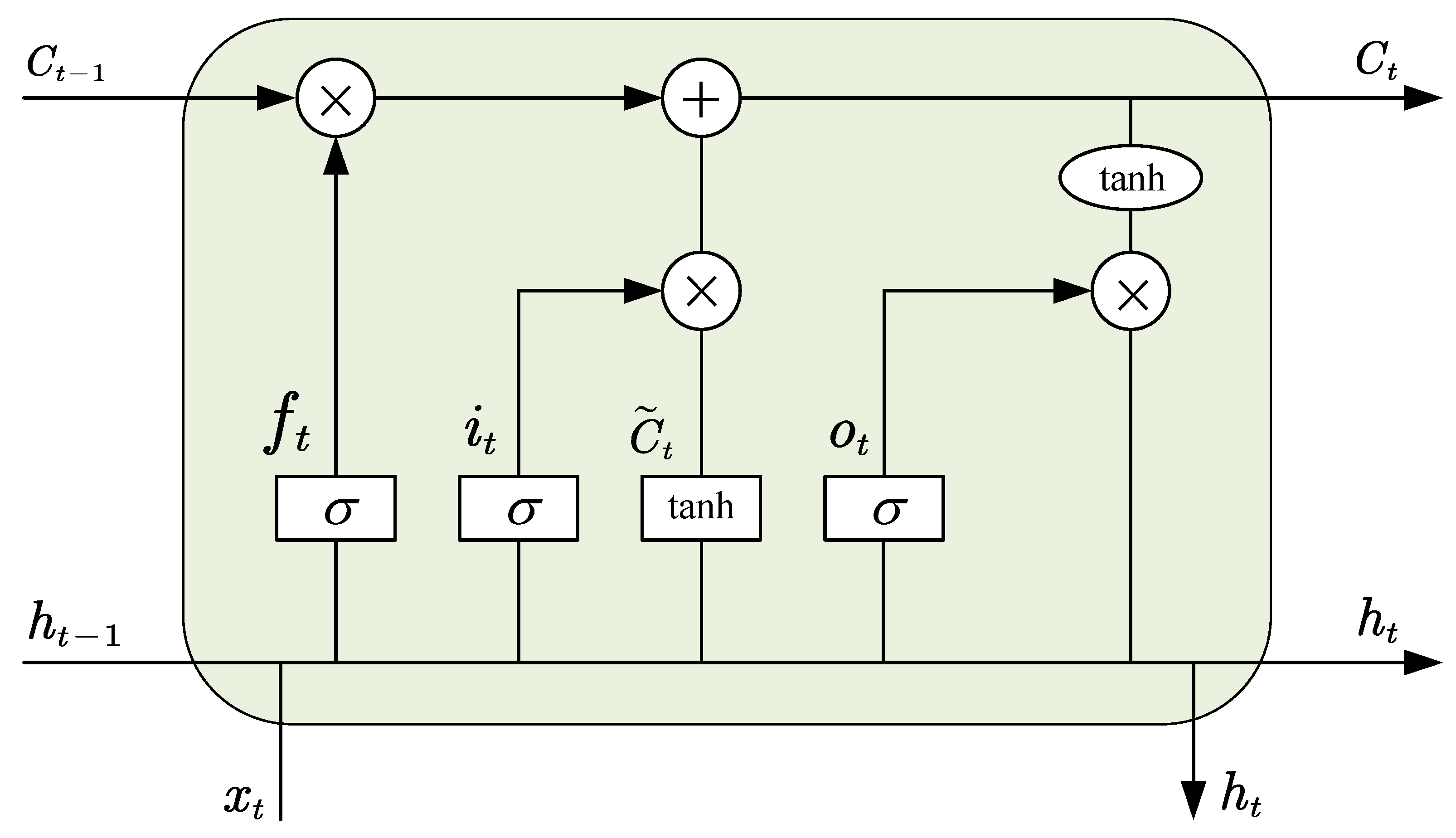
4.2. Long Short-Term Memory Networks

In a traditional neural networks model, it is fully connected between each layers but it is disconnected between the nodes in each layer [45]. As a result, it is inefficient for handling sequence problems. As mentioned above, the PW and BP data are both a time sequence. Accordingly, Recurrent Neural Networks (RNN) can be used for prediction. The nodes in the hidden layer of RNN are connected, which is different from traditional neural networks. What is more, the input of the hidden layer includes not only the output of the input layer, but also the output of the hidden layer of the previous time slot. The recurrent connections of RNN can add feedback and memory to the network over time. In summary, RNN has a strong learning ability and input generalization ability for sequence problems.

However, when back-propagation is used in a very deep RNN, the gradient of the neural network may become unstable, which will cause the exploding gradient problem or vanishing gradient problem [46], hence making the generated model unreliable. These problems can be solved by Long Short-Term Memory (LSTM) networks. As a variant of RNN, LSTM is composed of memory units and several gates. In Figure 1, we describe the structure of the LSTM unit.

In time slot t, we presume that the input and the output are $x_t$ and $h_t$, respectively. There are three gates in each unit, called input gate i, forget gate f and output o. The values of the three gates are calculated as follows:

$$f_t=\sigma (W_f·[h_{t-1},x_t]+b_f),$$

(5)

$$i_t=\sigma (W_i·[h_{t-1},x_t]+b_i),$$

(6)

$$o_t=\sigma (W_o·[h_{t-1},x_t]+b_o),$$

(7)

where $W_f$, $W_i$, $W_o$, $b_f$, $b_i$, $b_o$ are the correlative weight matrices and variable biases.

Then, the process of information updating in LSTM unit is as follows. In time slot t, the forget gate decides which part of $C_{t-1}$ to drop, according to $f_t·C_{t-1}$. The input gate decides what information to store in the unit, according to $i_t·{\tilde{C}}_t$, and ${\tilde{C}}_t$ is calculated as follows:

$${\tilde{C}}_t=tanh(W_c·[h_{t-1},x_t]+b_c),$$

(8)

where $W_c$ and $b_c$ are the weight matrix and variable bias of the memory unit. In this way, the current unit is updated as follows:

$$C_t=f_t·C_{t-1}+i_t·\widetilde{C_t},$$

(9)

in addition, the output data are calculated by the following:

$$h_t=o_t·tanh\left(C_t\right),$$

(10)

after that, $h_t$ and $C_t$ pass to the next cell in the next time slot. In conclusion, each unit works like a state machine in which three gates have their own weights, so that LSTM can deal with sequence problems better.

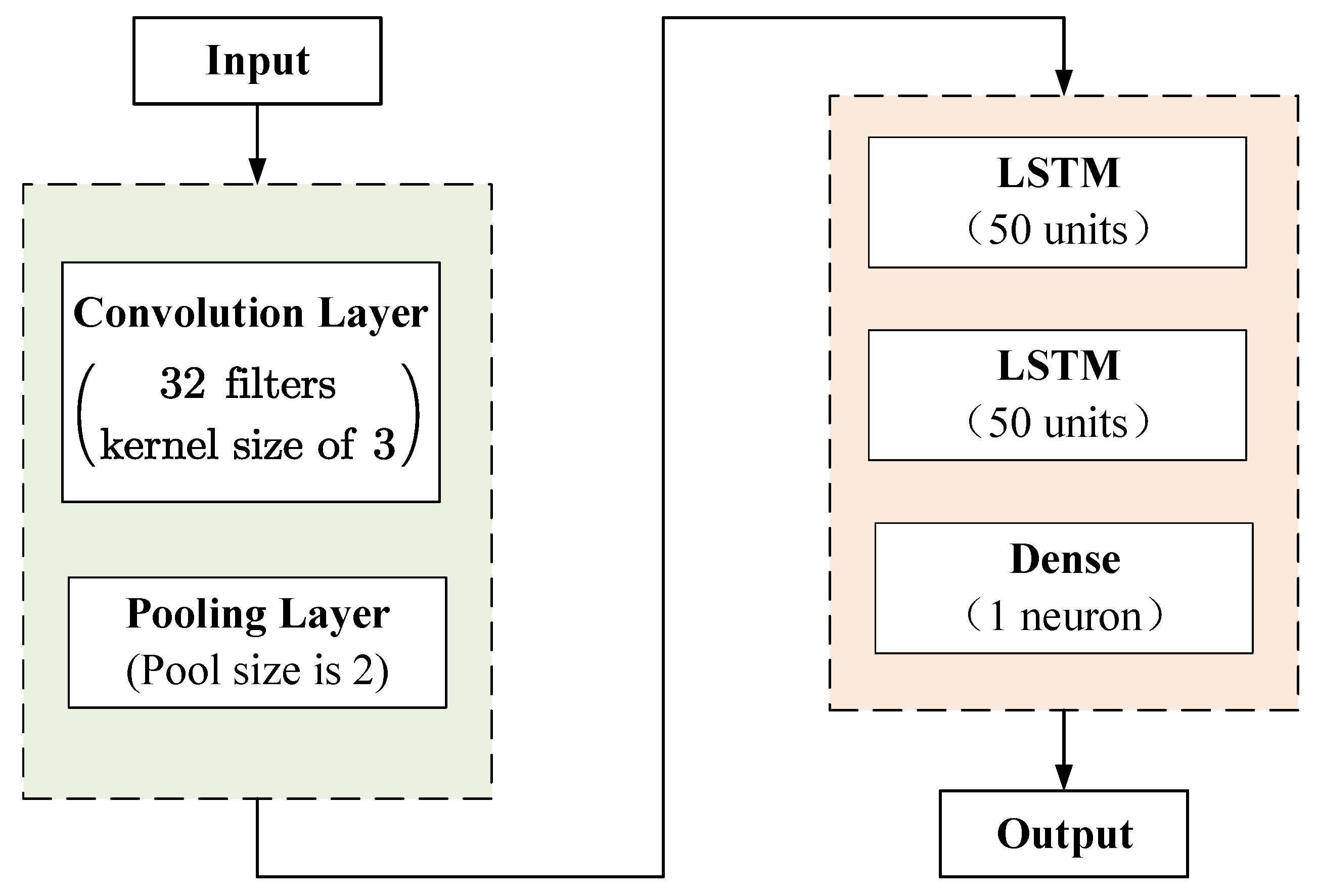
4.3. CNN-LSTM Prediction Method

As mentioned above, we use a hybrid model that consists of CNN and LSTM to predict BP values based on PW data. After the PW data are input, the features extraction is performed by CNN first. Then, the features are input into LSTM for further training. The topology of proposed model is shown in Figure 2.

In order to improve the accuracy of the BP prediction, we use the PW data of multiple recent time slots to predict the BP values of the next time slot, which is called the windows prediction method. As a result, we need to correlate the input data and output data to generate a data set for training and validation.

Subsequently, we use zero-mean (z-score) normalization to standardize the PW and BP data. Assume that the data are denoted by $\mathcal{X}=\{x^1,x^2,\dots ,x^t,\dots ,x^T\}$, for each input data $x^t$. The idea of z-score normalization is shown in Equation (11):

$$z^t=\frac{x^t-x_{mean}^t}{x_{std}^t},$$

(11)

where $x_{mean}^t$ is the mean value of $\mathcal{X}$ and $x_{std}^t$ are the standard deviation of $\mathcal{X}$. The mean of the processed data is 0, and the standard deviation is 1.

Notice that there are $n_w$ data in the input of the model, which will increase the complexity of the model. Furthermore, as $n_w$ boosts, the features in the input become sparse and difficult to extract. Hence, we use CNN to extract features from the PW data. In detailed, a convolutional layer with 32 filters and a kernel size of 3 is added, followed by a pooling layer with a pool size of 2 for further subsampling, which adopts the max pooling. At this point, the input features are successfully extracted and are more streamlined than the original input data.

Then, the features are passed to two LSTM hidden layers for further training, and each hidden layer has 50 units. Since the BP prediction problem is a regression problem, we use the dense layer (i.e., fully connected layer) with one neuron to receive the tensor from the LSTM hidden layer and output the BP value. Finally, the output is the predicted BP values. As a result, the proposed method is more efficient for the prediction of BP, due to the combination of the feature extraction capability of CNN with the advantage of LSTM for the time sequence.

5. Numerical Results and Performance Analysis

In this section, we evaluate the performance of proposed CNN-LSTM prediction method via numerical results.

5.1. Benchmarks and Parameter Settings

As mentioned above, the PW and BP data used in this work come from the Multi-parameter Intelligent Monitoring in Intensive Care (MIMIC) data set, which collects physiological data of over 90 patients in ICU. The sampling frequency of the data is 500 Hz. As shown in

Table 1. Data samples of the MIMIC data set.

Time and Data	III (mV)	ABP (mmHg)	PLETH (mV)	RESP (mV)
01:29:37.000 22/10/1994	−0.029	77.95	0.443	−0.464
01:29:37.002 22/10/1994	−0.032	77.95	0.443	−0.464
01:29:37.004 22/10/1994	−0.034	77.95	0.443	−0.464
01:29:37.006 22/10/1994	−0.036	77.95	0.443	−0.464
01:29:37.008 22/10/1994	−0.037	75.55	0.38	−0.467
...	...	...	...	...

, the PW data (PLETH) are obtained by fingertip pulse oximeter, and the unit is millivolt (mV). The BP data used in this paper are the arterial blood pressure (ABP), and the unit is millimeter of mercury (mmHg). MIMIC also includes ECG (III) and respiration (RESP) data, which are not used in our work. We selected the first three patients (their numbers in the data set are 39, 41, 55) in the MIMIC data set in our work, and the length of the data of each patient is 30,000 time slots (10 min in total).

In order to evaluate the performance of the proposed prediction method, we set the following five benchmarks, which is shown in

Table 2. Proposed prediction method and the setup of benchmarks.

Proposed Prediction Method and Benchmarks
Group 1	MLP	Only use multi-layer perceptron (MLP) for prediction.
	RNN	Only use recurrent neural networks (RNN) for prediction.
	LSTM	Only use LSTM for prediction.
Group 2	CNN-MLP	Combine CNN with MLP for prediction.
	CNN-RNN	Combine CNN with RNN for prediction.
	CNN-LSTM	Combine CNN with LSTM for prediction.

. Obviously, the proposed method and benchmarks can be classified into two groups. Group 1 contains MLP, RNN, and LSTM, which only uses neural networks for prediction. Group 2 contains CNN-MLP (i.e., the classic CNN network.), CNN-RNN, and CNN-LSTM, which uses CNN to extract features first. We use group 1 to figure out the most suitable neural networks for sequence problems, and group 2 shows the effect of CNN on the prediction accuracy.

For parameters settings of the neural networks, we set the number of input layer nodes to be related to the window length $n_w$. There is one hidden layer of each method, and the number of units of the hidden layers are all set to 50. The training epoch is set to 100. PW and BP data are divided into the training set and validation set, according to the order of the time series. The training set and validation set account for $70\%$ and $30\%$, respectively.

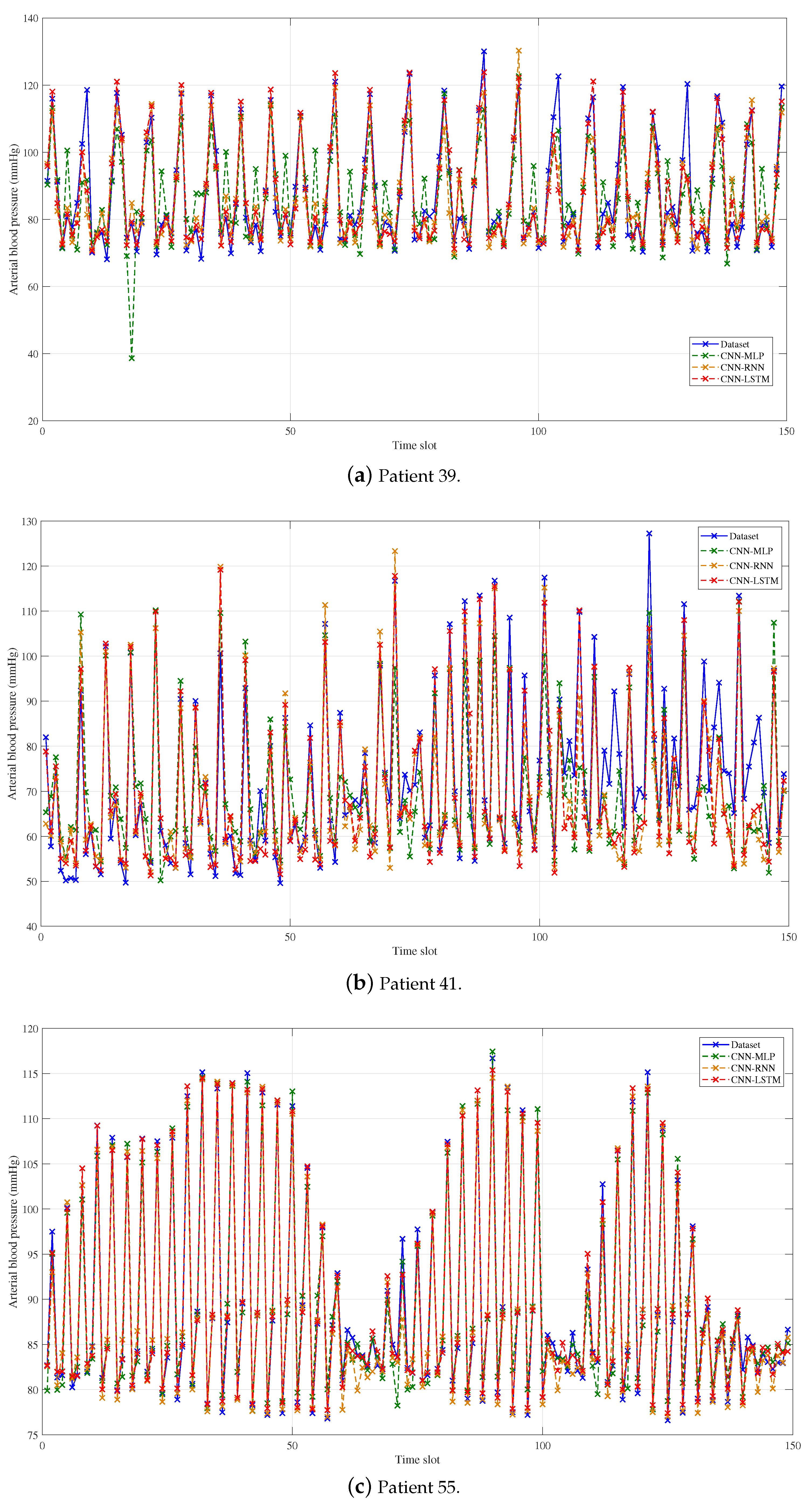
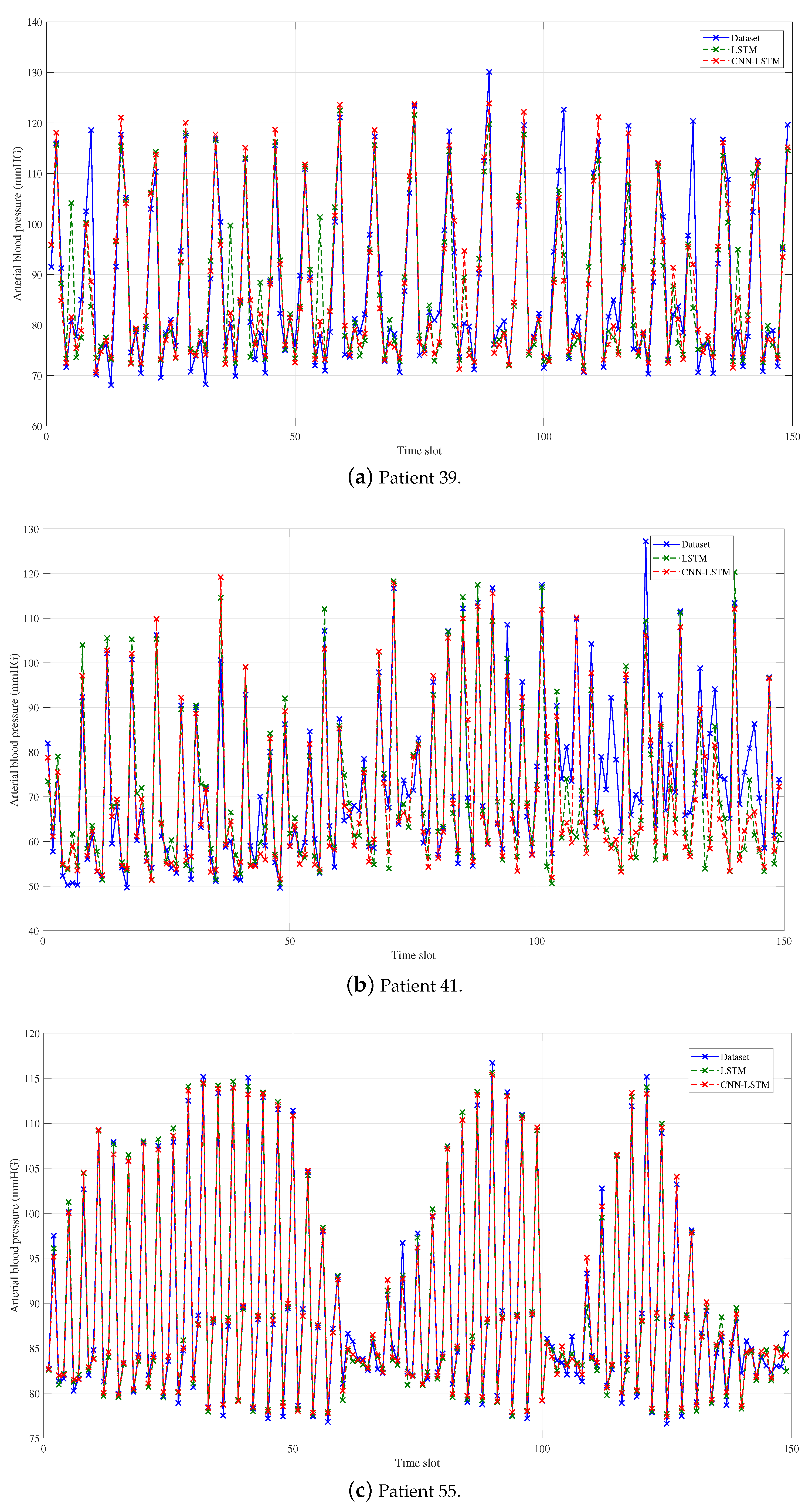
5.2. Results and Analysis

In order to evaluate the performance of the proposed prediction method, we introduce three evaluation indexes, including the mean absolute error (MAE), the mean absolute percent error (MAPE), and the root mean square error (RMSE). The definitions of the three evaluation indexes are as follows:

$$MAE=\frac{1}{n}\sum _{i=1}^n|{\widehat{y}}_i-y_i|,$$

(12)

$$MAPE=\frac{100\%}{n}\sum _{i=1}^n\left|\frac{{\widehat{y}}_i-y_i}{y_i}\right|,$$

(13)

$$RMSE=\sqrt{\frac{1}{n}\sum _{i=1}^n{({\widehat{y}}_i-y_i)}^2},$$

(14)

where ${\widehat{y}}_i$ is the prediction values, and $y_i$ is the real values, respectively.

We make a decimation of the original and the predicted data with the decimation factor of 200 in order to show the predicted performance more clearly, which is shown in Figure 3, Figure 4 and Figure 5. What is more, the average predicted performance of all methods is shown in

Table 3. Average predicted performance of patients.

Methods		MAE (mmHg)	MAPE (%)	RMSE (mmHg)	Training Time (s)
MLP	Train	4.61	5.76	6.43	120.92
	Val	5.66	6.77	7.62
RNN	Train	3.54	4.43	5.34	331.57
	Val	4.90	5.88	6.80
LSTM	Train	3.20	4.01	4.96	632.15
	Val	4.67	5.66	6.58
CNN-MLP	Train	5.00	6.34	6.73	142.87
	Val	5.65	6.68	7.50
CNN-RNN	Train	3.20	4.03	4.67	1006.11
	Val	4.78	5.80	6.37
CNN-LSTM	Train	2.37	3.04	3.53	337.15
	Val	4.42	5.43	6.01

, and the evaluation indexes of all methods are shown in

Table 4. Predicted performance of patient 39.

Methods		MAE (mmHg)	MAPE (%)	RMSE (mmHg)	Training Time (s)
MLP	Train	5.68	6.46	8.12	115.36
	Val	5.94	6.61	8.58
RNN	Train	4.27	4.76	7.02	321.87
	Val	4.54	4.95	7.44
LSTM	Train	3.82	4.30	6.49	648.72
	Val	4.18	4.60	6.96
CNN-MLP	Train	6.51	7.45	8.89	136.92
	Val	6.64	7.41	9.11
CNN-RNN	Train	3.62	4.11	5.58	1016.40
	Val	4.10	4.53	6.33
CNN-LSTM	Train	2.85	3.26	4.62	347.08
	Val	3.57	3.98	6.10

,

Table 5. Predicted performance of patient 41.

Methods		MAE (mmHg)	MAPE (%)	RMSE (mmHg)	Training Time (s)
MLP	Train	6.43	8.91	8.88	117.94
	Val	9.25	11.69	11.93
RNN	Train	5.32	7.37	7.68	341.55
	Val	9.10	11.47	11.52
LSTM	Train	4.90	6.73	7.20	600.85
	Val	8.96	11.39	11.53
CNN-MLP	Train	7.00	9.85	9.38	147.11
	Val	8.76	10.85	11.46
CNN-RNN	Train	4.78	6.62	6.70	942.44
	Val	9.09	11.56	11.01
CNN-LSTM	Train	3.41	4.86	4.72	328.31
	Val	8.02	10.24	10.05

and

Table 6. Predicted performance of patient 55.

Methods		MAE (mmHg)	MAPE (%)	RMSE (mmHg)	Training Time (s)
MLP	Train	1.73	1,90	2.29	129.46
	Val	1.80	2.00	2.34
RNN	Train	1.02	1.15	1.32	331.29
	Val	1.06	1.21	1.43
LSTM	Train	0.87	0.99	1.20	646.88
	Val	0.87	0.99	1.26
CNN-MLP	Train	1.50	1.71	1.91	144.58
	Val	1.54	1.77	1.93
CNN-RNN	Train	1.20	1.35	1.73	1059.49
	Val	1.16	1.31	1.78
CNN-LSTM	Train	0.78	0.89	1.05	339.25
	Val	0.85	0.97	1.23

. In general, the predicted BP values of all methods fit the original values of data set very well, and the evaluation is also acceptable as compared to the current methods, which proves the effectiveness of BP prediction based on PW data. Obviously, our proposed CNN-LSTM prediction method has the best performance among all methods, and there are some results worth noting.

As shown in Figure 3, group 1 shows that, without the help of CNN, LSTM has the best predictive performance of all evaluation indexes, while it requires the longest training time. Compared with MLP, LSTM can improve the training set MAE of three patients to $32.75\%$, $23.79\%$ and $49.71\%$, and can improve the validation set to $29.63\%$, $3.78\%$ and $51.67\%$. The training time of LSTM is more than 5 times that of MLP. That is because LSTM has a strong ability to deal with time sequences, but the network structure of LSTM is more complicated than that of MLP.

When we focus on group 2 in Figure 4, CNN-LSTM still has the best performance compared to other CNN-assisted methods. Compared with CNN-RNN, CNN-LSTM can improve the training set MAE to $21.27\%$, $28.66\%$ and $35\%$, and can improve the validation set to $12.93\%$, $11.77\%$ and $26.72\%$. Interestingly, the training time required for CNN-LSTM is lower than that of CNN-RNN by $65.85\%$, $65.15\%$ and $67.98\%$, respectively. The reason for the long training time of CNN-RNN is the deterioration in learning speed, which is caused by the unstable gradient problem, that is, the exploding gradient or vanishing gradient problem mentioned above.

When comparing the indexes between group 1 and group 2 in Figure 5, we can clearly find that combining neural networks with CNN can effectively improve the prediction performance. Remember that we set the window length $n_w$ to 20, i.e., the PW data of 20 time slots (40 ms) are entered into the network. The data are also spares, while containing useful information. Therefore, the filters in the convolution layer first extract features from the input data. Then, the pooling layer further subsamples the features before entering into the LSTM layers. As a result, LSTM accounts for the time correlation of the feature, which is better than directly considering the time correlation in the input data. That is because the information in the features is more concise and effective than the original input data. Specifically, compared with LSTM, CNN-LSTM can improve the training set MAE of three patients to $25.39\%$, $30.41\%$ and $10.34\%$, respectively. For the validation set, the improvements of MAE are $14.59\%$, $10.49\%$ and $2.30\%$. Additionally, the proposed method is a kind of end-to-end network and does not need to be trained separately. Effective feature extraction reduces the training time of the three patients, compared to LSTM, to $48.02\%$, $45.36\%$ and $47.56\%$. The numerical results prove the effectiveness of the proposed CNN-LSTM prediction method.

However, combining CNN with neural networks, especially MLP and RNN, does not necessarily improve the predicted performance. In Table 5, the performance of CNN-MLP on the training set is worse than MLP. Combining CNN with MLP is equivalent to classic Convolutional Neural Networks, which is usually used for image recognition rather than data prediction. In other words, the features extracted by CNN cannot be well learned by following MLP. In Table 6, CNN-RNN has worse performance than RNN in both the training set and validation set, which is caused by unstable gradient problem. These results confirm the correctness and effectiveness of the proposed CNN-LSTM method once again.

6. Conclusions and Discussion

In this paper, we have proposed a novel CNN-LSTM predicted model of blood pressure (BP) based on pulse wave (PW) data. In the CNN-LSTM model, a convolutional layer and a pooling layer are used to extract features from PW data. Then two LSTM hidden layers are used for further training. We set two groups of benchmarks. The experiment results based on the MIMIC data set show that the proposed method is close to or better than the existing BP estimation methods. In particular, the proposed method can significantly improve the predicted accuracy by up to $30.41\%$ while saving training time, due to combining the advantages of CNN and LSTM.

However, we need to train multiple models to perform BP prediction on different patients in our current work, which cannot be widely used for a large number of patients. In the future, we will consider introducing the state-of-art technologies in the area of AI, e.g., transfer learning, to improve the generalization ability of the model. According to place the generalized model in portable devices which can receive PW data from the fingertip pulse oximeter, we can provide convenient and real-time BP monitoring for a wider range of people.

References

1. Nabel, E.G. Cardiovascular disease. N. Engl. J. Med. 2003, 349, 60–72. [Google Scholar] [CrossRef] [PubMed]
2. Al-Absi, H.R.H.; Refaee, M.A.; Rehman, A.U.; Islam, M.T.; Belhaouari, S.B.; Alam, T. Risk factors and comorbidities associated to cardiovascular disease in Qatar: A machine learning based case-control study. IEEE Access 2021, 9, 29929–29941. [Google Scholar] [CrossRef]
3. Mancia, G.; Sega, R.; Milesi, C.; Cessna, G.; Zanchetti, A. Blood-pressure control in the hypertensive population. Lancet 1997, 349, 454–457. [Google Scholar] [CrossRef]
4. SPRINT Research Group. A randomized trial of intensive versus standard blood-pressure control. N. Engl. J. Med. 2015, 373, 2103–2116. [Google Scholar] [CrossRef]
5. Mahmood, S.N.; Ercelecbi, E. Development of blood pressure monitor by using capacitive pressure sensor and microcontroller. In Proceedings of the International Conference on Engineering Technology and their Applications (IICETA), Al-Najaf, Iraq, 8–9 May 2018; pp. 96–100. [Google Scholar]
6. Zakrzewski, A.M.; Huang, A.Y.; Zubajlo, R.; Anthony, B.W. Real-time blood pressure estimation from force-measured ultrasound. IEEE Trans. Biomed. Eng. 2018, 65, 861. [Google Scholar] [CrossRef] [PubMed]
7. Parasuraman, S.; Raveendran, R. Measurement of invasive blood pressure in rats. J. Pharmacol. Pharmacother. 2012, 3, 172. [Google Scholar]
8. Takci, S.; Yigit, S.; Korkmaz, A.; Yurdakök, M. Comparison between oscillometric and invasive blood pressure measurements in critically ill premature infants. Acta Paediatr. 2012, 101, 132–135. [Google Scholar] [CrossRef]
9. Sebald, D.J.; Bahr, D.E.; Kahn, A.R. Narrowband auscultatory blood pressure measurement. IEEE Trans. Biomed. Eng. 2002, 49, 1038–1044. [Google Scholar] [CrossRef]
10. Sapinski, A. Standard algorithm of blood-pressure measurement by the oscillometric method. Med. Biol. Eng. Comput. 1992, 30, 671. [Google Scholar] [CrossRef]
11. Hirata, K.; Kawakami, M.; O’Rourke, M.F. Pulse wave analysis and pulse wave velocity a review of blood pressure interpretation 100 years after Korotkov. Circ. J. 2006, 70, 1231–1239. [Google Scholar] [CrossRef] [Green Version]
12. Chen, Y.; Wen, C.; Tao, G.; Bi, M.; Li, G. Continuous and noninvasive blood pressure measurement: A novel modeling methodology of the relationship between blood pressure and pulse wave velocity. Ann. Biomed. Eng. 2009, 37, 2222–2233. [Google Scholar] [CrossRef] [PubMed]
13. Avolio, A.P.; Butlin, M.; Walsh, A. Arterial blood pressure measurement and pulse wave analysis—Their role in enhancing cardiovascular assessment. Physiol. Meas. 2009, 31, R1–R47. [Google Scholar] [CrossRef] [PubMed]
14. Tanaka, H.; Sakamoto, K.; Kanai, H. Indirect blood pressure measurement by the pulse wave velocity method. Jpn. J. Med. Electron. Biol. Eng. 1984, 22, 13–18. [Google Scholar]
15. Wibmer, T.; Kropf, C.; Stoiber, K.; Ruediger, S.; Lanzinger, M.; Rottbauer, W.; Schumann, C. Pulse transit time and blood pressure during cardiopulmonary exercise tests. Physiol. Res. 2014, 63, 287. [Google Scholar] [CrossRef] [PubMed]
16. Fortin, J.; Rogge, D.E.; Fellner, C.; Flotzinger, D.; Saugel, B. A novel art of continuous noninvasive blood pressure measurement. Nat. Commun. 2021, 12, 1387. [Google Scholar] [CrossRef] [PubMed]
17. Peltokangas, M.; Vehkaoja, A.; Verho, J.; Mattila, V.M.; Romsi, P.; Lekkala, J.; Oksala, N. Age dependence of arterial pulse wave parameters extracted from dynamic blood pressure and blood volume pulse waves. IEEE J. Biomed. Health Inform. 2017, 21, 142–149. [Google Scholar] [CrossRef] [PubMed]
18. Liu, S.; Lai, S.; Wang, J.; Tan, T.; Huang, Y. The cuffless blood pressure measurement with multi-dimension regression model based on characteristics of pulse waveform. In Proceedings of the 41st Annual International Conference of the IEEE Engineering in Medicine and Biology Society (EMBC), Berlin, Germany, 23–27 July 2019; pp. 6838–6841. [Google Scholar]
19. Singla, M.; Sistla, P.; Azeemuddin, S. Cuff-less blood pressure measurement using supplementary ECG and PPG features extracted through wavelet transformation. In Proceedings of the 41st Annual International Conference of the IEEE Engineering in Medicine and Biology Society (EMBC), Berlin, Germany, 23–27 July 2019; pp. 4628–4631. [Google Scholar]
20. Raschman, E.; Durackova, D. New digital architecture of CNN for pattern recognition. In Proceedings of the MIXDES-16th International Conference Mixed Design of Integrated Circuits and Systems, Lodz, Poland, 25–27 June 2009; pp. 662–666. [Google Scholar]
21. Gu, J.; Wang, Z.; Kuen, J.; Ma, L.; Shahroudy, A.; Shuai, B.; Chen, T. Recent advances in convolutional neural networks. Pattern Recognit. 2018, 77, 354–377. [Google Scholar] [CrossRef] [Green Version]
22. Sainath, T.N.; Mohamed, A.; Kingsbury, B.; Ramabhadran, B. Deep convolutional neural networks for LVCSR. In Proceedings of the IEEE International Conference on Acoustics, Speech and Signal Processing, Vancouver, BC, Canada, 26–31 May 2013; pp. 8614–8618. [Google Scholar]
23. Liao, S.; Wang, J.; Yu, R.; Sato, K.; Cheng, Z. CNN for situations understanding based on sentiment analysis of twitter data. Procedia Comput. Sci. 2017, 111, 376–381. [Google Scholar] [CrossRef]
24. Luo, H.; Xiong, C.; Fang, W.; Love, P.E.; Zhang, B.; Ouyang, X. Convolutional neural networks: Computer vision-based workforce activity assessment in construction. Autom. Constr. 2018, 94, 282–289. [Google Scholar] [CrossRef]
25. Khan, S.; Rahmani, H.; Shah, S.A.A.; Bennamoun, M. A guide to convolutional neural networks for computer vision. Synth. Lect. Comput. Vis. 2018, 8, 1–207. [Google Scholar] [CrossRef]
26. Graves, A. Long short-term memory. In Supervised Sequence Labelling with Recurrent Neural Networks; Springer: Berlin, Germany, 2012; pp. 37–45. [Google Scholar]
27. Mou, H.; Liu, Y.; Wang, L. LSTM for Mobility Based Content Popularity Prediction in Wireless Caching Networks. In Proceedings of the IEEE Globecom Workshops (GC Wkshps), Waikoloa, HI, USA, 9–13 December 2019; pp. 1–6. [Google Scholar]
28. Graves, A.; Jaitly, N.; Mohamed, A. Hybrid speech recognition with Deep Bidirectional LSTM. In Proceedings of the IEEE Workshop on Automatic Speech Recognition and Understanding, Olomouc, Czech Republic, 8–12 December 2013; pp. 273–278. [Google Scholar]
29. Zeyer, A.; Doetsch, P.; Voigtlaender, P.; Schlüter, R.; Ney, H. A comprehensive study of deep bidirectional LSTM RNNs for acoustic modeling in speech recognition. In Proceedings of the IEEE International Conference on Acoustics, Speech and Signal Processing (ICASSP), New Orleans, LA, USA, 5–9 March 2017; pp. 2462–2466. [Google Scholar]
30. Zhao, Z.; Chen, W.; Wu, X.; Chen, P.C.; Liu, J. LSTM network: A deep learning approach for short-term traffic forecast. IET Intell. Transp. Syst. 2017, 11, 68–75. [Google Scholar] [CrossRef] [Green Version]
31. Liu, Y.; Guan, L.; Hou, C.; Han, H.; Liu, Z.; Sun, Y.; Zheng, M. Wind power short-term prediction based on LSTM and discrete wavelet transform. Appl. Sci. 2019, 9, 1108. [Google Scholar] [CrossRef] [Green Version]
32. Wang, J.; Yu, L.C.; Lai, K.R.; Zhang, X. Dimensional sentiment analysis using a regional CNN-LSTM model. In Proceedings of the 54th Annual Meeting of the Association for Computational Linguistics, Berlin, Germany, 7–12 August 2016; pp. 225–230. [Google Scholar]
33. Kim, T.Y.; Cho, S.B. Predicting residential energy consumption using CNN-LSTM neural networks. Energy 2019, 182, 72–81. [Google Scholar] [CrossRef]
34. Miao, F.; Wen, B.; Hu, Z.; Fortino, G.; Li, Y. Continuous blood pressure measurement from one-channel electrocardiogram signal using deep-learning techniques. Artif. Intell. Med. 2020, 108, 101919. [Google Scholar] [CrossRef]
35. Eom, H.; Lee, D.; Han, S.; Hariyani, Y.S.; Lim, Y.; Sohn, I.; Park, K.; Park, C. End-To-End Deep Learning Architecture for Continuous Blood Pressure Estimation Using Attention Mechanism. Sensors 2020, 20, 2338. [Google Scholar] [CrossRef] [Green Version]
36. Zhang, Y.; Wang, Z. A hybrid model for blood pressure prediction from a PPG signal based on MIV and GA-BP neural network. In Proceedings of the 13th International Conference on Natural Computation, Fuzzy Systems and Knowledge Discovery (ICNC-FSKD), Chongqing, China, 12–14 June 2020; pp. 1989–1993. [Google Scholar]
37. Chen, Y.; Cheng, J.; Ji, W. Continuous blood pressure measurement based on photoplethysmography. In Proceedings of the 14th IEEE International Conference on Electronic Measurement and Instruments (ICEMI), Guilin, China, 29–31 July 2017; pp. 1656–1663. [Google Scholar]
38. Chen, X.; Yu, S.; Zhang, Y.; Chu, F.; Sun, B. Machine Learning Method for Continuous Noninvasive Blood Pressure Detection Based on Random Forest. IEEE Access 2021, 9, 34112–34118. [Google Scholar] [CrossRef]
39. Shimazaki, S.; Kawanaka, H.; Ishikawa, H.; Inoue, K.; Oguri, K. Cuffless blood pressure estimation from only the Waveform of photoplethysmography using CNN. In Proceedings of the 41st Annual International Conference of the IEEE Engineering in Medicine and Biology Society (EMBC), Berlin, Germany, 23–27 July 2019; pp. 5042–5045. [Google Scholar]
40. Sun, X.; Zhou, L.; Chang, S.; Liu, Z. Using CNN and HHT to predict blood pressure level based on photoplethysmography and its derivatives. Biosensors 2021, 11, 120. [Google Scholar] [CrossRef]
41. Zhao, Q.; Hu, X.; Lin, J.; Deng, X.; Li, H. A novel short-term blood pressure prediction model based on LSTM. AIP Conf. Proc. 2019, 2058, 020003. [Google Scholar]
42. Lo, F.P.W.; Li, C.X.T.; Wang, J.; Cheng, J.; Meng, M.Q.H. Continuous systolic and diastolic blood pressure estimation utilizing long short-term memory network. In Proceedings of the 39th Annual International Conference of the IEEE Engineering in Medicine and Biology Society (EMBC), Jeju, Korea, 23–27 July 2017; pp. 1853–1856. [Google Scholar]
43. Tanveer, M.S.; Hasan, M.K. Cuffless blood pressure estimation from electrocardiogram and photoplethysmogram using waveform based ANN-LSTM network. Biomed. Signal Process. Control. 2019, 51, 382–392. [Google Scholar] [CrossRef] [Green Version]
44. Moody, G.B.; Mark, R.G. A database to support development and evaluation of intelligent intensive care monitoring. In Proceedings of the Computers in Cardiology, Indianapolis, IN, USA, 8–11 September 1996; pp. 657–660. [Google Scholar]
45. MacKay, D.J.C. A practical Bayesian framework for backpropagation networks. IEEE Trans. Netw. Sci. Eng. 1992, 4, 448–472. [Google Scholar] [CrossRef]
46. Tsai, K.C.; Wang, L.; Han, Z. Caching for mobile social networks with deep learning: Twitter analysis for 2016 U.S. election. IEEE Trans. Netw. Sci. Eng. 2020, 7, 193–204. [Google Scholar] [CrossRef]
Figure 1. The structure of LSTM unit [27].
Electronics 10 01664 g001
Figure 2. The topology of the CNN-LSTM model.
Electronics 10 01664 g002
Figure 3. Prediction results of group 1: MLP, RNN, and LSTM.
Electronics 10 01664 g003
Figure 4. Prediction results of Group 2: CNN-MLP, CNN-RNN, and CNN-LSTM.
Electronics 10 01664 g004
Figure 5. Prediction results of LSTM and CNN-LSTM.
Electronics 10 01664 g005